Towards In-Field Phenotyping Exploiting Differentiable Rendering with Self-Consistency Loss
←
→
Page content transcription
If your browser does not render page correctly, please read the page content below
Towards In-Field Phenotyping
Exploiting Differentiable Rendering with Self-Consistency Loss
Federico Magistri Nived Chebrolu Jens Behley Cyrill Stachniss
Abstract— In modern agriculture, measuring phenotypic
traits helps breeders monitor plant growth, increase yield, and
provide food, feed, and fiber. Traditional phenotyping requires
intensive manual work, partially being intrusive. In this paper,
we investigate the challenge of measuring phenotypic traits in
an automated fashion through mobile robots operating in field
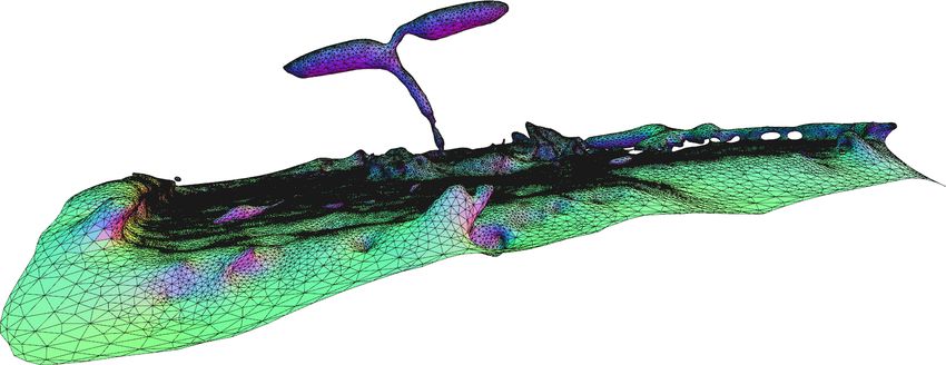
environments. In particular, we want to measure plants from (a) Manually obtained point cloud with a high-precision scanner
images acquired by mobile robots instead of using data from a
static scanning environment. We propose to use a differentiable
rendering approach to deform a generic 3D template of a plant
to fit the observation recorded by a robot while ensuring a
coherent deformation of the plant template. The experiments
presented in this paper suggest that our approach allows for
3D reconstruction of different plant species at different growth
stages using single images. From that model, we can compute (b) Point cloud obtained with a robotic platform
important phenotypic traits, such as the leaf area index.
I. I NTRODUCTION
Phenotyping is the task of measuring plant traits to de-
scribe plant physiology and it is central in plant science. Also
breeders use phenotyping measurements to support decisions
in crop fields. Such decisions include selecting the best (c) Results of our approach
cultivars to continue the breeding process and selecting the Fig. 1: To measure phenotypic traits, it is fundamental to obtain
best cultivars for the following seasons. Phenotyping, how- 3D data of plants with high spatial resolution. Yet, state-of-the-art
ever, is expensive, time-consuming, and requires intrusive approaches, either registration or reconstruction algorithms, are not
operations that potentially damages the crop. Phenotyping sufficient for accurate phenotyping at a plant level. As an example,
the top row shows the point cloud obtained with a hand-held laser
is mostly performed during the plant breeding process, and scanner, the middle row shows the same scene captured with a depth
in this context, mobile robots equipped with sensors and camera. Our goal is to infer the 3D geometry of plants using single
data interpretation capabilities have the potential to become images shown in the bottom row depicting the triangle meshes
a game-changer [8], [7]. reconstructed with our approach.
In recent years, there has been an increase in studies em-
ploying robots in fields. The majority of those works exploit
approaches employ a flatbed scanner to measure the leaf area.
sensor data to tackle tasks such as weeding [21], [10], [25],
This approach is not suited for large-scale monitoring since
[36], crop counting [18], [39], or fruit picking [19]. Fewer
humans have to measure each leaf in the field manually. In
works exploit robots to measure phenotypic traits based on
the past years, several studies presented a way to measure
the complete 3D plant geometry, which are important to
the leaf areas. These approaches, however, require highly ac-
evaluate crop health. Existing approaches often measure only
curate 3D point clouds of plants to measure such phenotypic
basic traits such as crop height [3], [4] when operating in the
traits [41], [40], [9], [11].
field and outside greenhouses.
This paper tackles estimating important phenotypic traits, In the agricultural setting, obtaining high-fidelity point
such as the leaf area, through mobile robots, using regular clouds is challenging due to the high level of details needed.
2D camera images instead of costly 3D reconstruction set- For example, Fig. 1 illustrates the differences between a point
tings. Measuring the leaf area, for example, is an important cloud obtained with a high-precision laser scanner and with
estimator of a plant’s capability to capture sunlight. Current human support (top row) and a point cloud obtained with
a robotic onboard depth camera (middle row). One can see
All authors are with the University of Bonn, Germany. the challenges of in-field phenotyping, such as noisy and
This work has been funded by the Deutsche Forschungsgemeinschaft
(DFG, German Research Foundation) under Germany’s Excellence Strategy, incomplete data that make the phenotypic evaluation of traits
EXC-2070 – 390732324 (PhenoRob) and by the Federal Ministry of at a plant level inaccurate. Our goal is to recover the 3D
Food and Agriculture (BMEL) based on a decision of the Parliament of geometry of plants using only 2D images and a database of
the Federal Republic of Germany via the Federal Office for Agriculture
and Food (BLE) under the innovation support programme under funding 3D templates of generic plants. The results of our approach
no 28DK108B20 (RegisTer). are shown in the bottom row.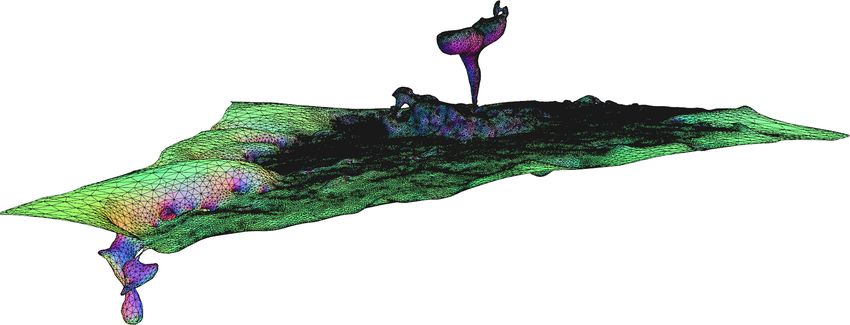
Deformed Template

                                   Instance
                                 Segmentation
     Input
                    CNN
     Image                       Growth State
                                  Estimation

                                   Template
                                   Database
                                                                                                               Selected Template
Fig. 2: An overview of our approach. We use as a preprocessing step the work of Weyler et al. [35] that provides a pixel-wise instance
segmentation and an estimate of the BBCH index. Based on this estimate, we select a plant template P, in the form of a triangle mesh,
from our database. Our goal is to deform the template, P̂, such that it fits the current observation from the robot, I. This is possible by
combining a differentiable rendering module with notions borrowed from non-rigid registration literature. We first render our template
mesh, denoted as r(P̂), and then we deform it such that the rendered image r(P̂) and the input image I look similar, which is guided by
the reconstruction loss Lr . Additionally, we enforce local rigidity with a structural loss Lc that aims at maintaining the structure of the
plant template P with the deformed mesh P̂.

   The main contribution of this paper is a method to infer            their phenotype values involving sampling of parameterized
the 3D shape of plants using single 2D images. We exploit              3D plant models from an underlying probability distribution,
the prior knowledge about the structure of plants [28] at a            thus casting phenotyping as a search in the space of plant
given growth stage called BBCH index [12], by computing a              models. Our work is different in two aspects. First, we want
library of generic plant templates that we then modify. Given          to recover the 3D structure of the whole plant, not only its
such a library and the taken image of a plant, we select the           sub-units. Second, we use images as input instead of point
most appropriate template based on the BBCH index. We,                 clouds (we only use a 3D point cloud to compute plant
then, deform the selected plant template, with a differentiable        templates when building the template database). Potentially,
rendering approach, such that its rendered view aligns with            one could also define the template model using a computer
the target image. In this way, we can estimate phenotypic              graphics engine [6], thus removing entirely the need for
traits, such as the leaf area index (LAI) without the need for         capturing 3D data of plants.
costly 3D reconstruction nor human intervention.                          The task of estimating 3D shapes of plants can be seen
   In sum, our approach can (i) compute a simplified mesh              as a non-rigid registration problem. Non-rigid registration
given 3D point clouds to create a library of generic plant             techniques can register scans with localized deformations
templates, (ii) deform the selected plant template to fit              in contrast to rigid registration techniques such as iterative
the observation coming from a mobile robot to recover its              closest point (ICP). One can divide these approaches into
3D structure, and (iii) accurately measure leaf area on the            two categories. On one side, approaches that explicitly com-
deformed mesh targeting in-field applications. These claims            pute the data association between source and target point
are backed up by the paper and our experimental evaluation.            clouds [31], [42], [5]. On the other side, approaches that
                    II. R ELATED W ORKS                                cast the registration task as a probability density estimation
   Phenotyping using mobile robots is still limited to basic           problem [27], [26]. In both cases, source and target are
traits such as average plant height over the entire field. For         instances of 3D data. This is different in our case as we
example, the works by Carlone et al. [3] and by Chebrolu               deal with heterogeneous inputs: we try to align a 3D source
et al. [4], show point clouds of crop fields at different              mesh to a target image. We do that in a way such that the
growth stages. Using non-rigid registration techniques they            rendered view of the mesh aligns with the image.
can estimate how the height of the plants changes by                      Differentiable rendering can deal with such heterogeneity.
aligning the different point clouds. Additionally, a couple            In a nutshell, it defines an approximation of the standard
of works integrates prior knowledge of plant structures into           rasterization method such that it can be differentiated with
3D measurements. Binney et al. [1] fit cylinders to point              respect to different parameters, i.e., materials, illuminations,
clouds of trees to recover missing data. However, the most             camera poses, etc. [20]. In recent years, differentiable ren-
similar work to ours is Sodhi et al. [30], which addresses the         dering modules have been used on top of neural network
problem of mapping plant sub-units called plant phytomers to           frameworks for a variety of vision tasks such as view
SOMs are unsupervised neural networks using competitive
                                                                      learning instead of backpropagation. They take as input a grid
                                                                      that organizes itself to capture the topology of the input data.
                                                                      Given the input grid G and the input set P, in our case both
                                                                      G and P are composed of points in R3 , the SOM defines a
                                                                      fully-connected layer between G and P. The learning process
                                                                      is composed of two alternating steps until convergence. First,
                                                                      the winning unit is computed as the argmini ||x−wi ||, where
Fig. 3: An example of our 3D reconstruction (left) compared to
the state-of-the-art (right) Poisson reconstruction [14]. While the   x is a randomly chosen sample from P and wi is the weight
captured topology is similar, our approach has fewer vertices. In     vector most similar to x, also called best matching unit. The
this way, we simplify and speed up the optimization procedure.        second step consists of updating the weights of each unit
                                                                      according to wn = wn + η β(i) (x − wi ), where η is the
                                                                      learning rate and β(i) a function, which weights the distance
synthesis [24], relighting [23], or material estimation [29].         between unit n and the best matching unit. The SOM
For a complete overview of the subject, we refer to the               approach computes a simplified mesh with fewer vertices
state-of-the-art report by Tewari et al. [34]. The drawback           than the state-of-the-art method for 3D reconstruction such
of these approaches is the amount of data required for the            as Poisson [14]. The fewer number of vertices simplifies and
training and the lack of generalization capability. Therefore,        accelerates the optimization procedure while capturing the
we follow an approach without a learning step and use the             geometry of the considered plant well, see Fig. 3 for an
rendering definition of Kato et al. [13]. We couple it with           example.
ideas from the non-rigid registration domain, ensuring that
the deformed model maintains the topology and aspect of a             B. Differentiable Rendering
plant.                                                                   Given a 3D mesh, such as those present in the template
    Additionally, in human motion analysis, a large amount            database, we can define a differentiable rendering operator
of study deals with heterogeneous input where a human                 to compare the 3D template to the current observation of
skeleton is deformed to fit the target image [38]. Skeleton           the robot. With differentiable rendering, we want to generate
fitting of humans is possible since the skeleton structure            images from a parametrized mesh that not only provides a
does not change and the difference in the target pose can             rendered view of this mesh but also allows for differentiation
be determined with a kinematic chain of the skeleton [37],            with respect to the mesh vertices. In this way, we can
[2], [33]. We take the idea of skeleton fitting and extend it         determine how the mesh should be deformed to match the
to the agricultural scenario by computing a simplified mesh           desired goal.
that we deform using a differentiable rendering approach.                Using a differentiable renderer, we can define a loss
                                                                      function and use gradient descent to minimize such loss,
                     III. O UR A PPROACH                              exploiting modern machine learning frameworks to speed up
   Our approach takes as input single images from an on-              the optimization. We use the definition of the 3D mesh ren-
board camera and a library of generic plant templates. In             derer by Kato et al. [13]. We consider the value v of a pixel
this paper, we use few highly accurate point clouds of plants         as a function r of the mesh vertices, P = r(v). Representing
obtained with a laser scanner from which we extract a                 the displacement of a vertex vi as δiv = v1 − v0 , where
simplified 3D mesh that we use as a template. Our goal                v0 and v1 represent its extremes, and its corresponding
is to deform the template to fit the current observation of           change in the rendered value δir = r(v1 ) − r(v0 ). In the
the robot, thus enabling phenotypic measurements on the               standard rasterization method, the derivative ∂r(v)
                                                                                                                        ∂v    is zero
deformed mesh. See Fig. 2 for an overview of our approach.            almost everywhere, thus there will be no gradient flow in the
As a preprocessing step, we use the work of Weyler et al. [35]        backpropagation step. This is due to the fact that the value
that provides pixel-wise instance segmentation of plants and          of the pixel changes suddenly when the face that influences
an estimate of the BBCH index. i.e., its growth stage.                the rendered value changes.    To solve this issue, the deriva-
                                                                           ∂r(v)            δir
                                                                      tive ∂v becomes δv between v0 and v1 , representing a
A. Mesh Extraction for Building a Template Database                                          i
                                                                      gradual change in the considered displacement. Once the
   To define a library of generic plant templates, we use             differentiable renderer is defined, we can use it, paired with
few highly accurate 3D point clouds of plants. We compute             optimization algorithms developed in the context of deep
a triangle mesh representation for these plant templates              learning, to deform the source mesh by minimizing the norm
from the respective point clouds. This computation starts             between its rendered view and the target image, such that
by classifying each point in the point cloud as stem or one           rendered image will be as similar as possible to the target
leaf instance. This step is necessary as it will enable us to         image.
compute phenotypic traits afterward. Once the point cloud is
segmented, we compute a grid structure for each organ, i.e.,          C. Differentiable Rendering Meets Non-rigid Registration
stem or leaves, based on self-organizing maps (SOM) [17]                We are not interested in the rendered image as most
used in prior work [22].                                              rendering systems. Instead, we are interested in the deformed
Rendered
Selected
Template
Rendered
Deformed
Template
Semantically
Segmented
Input Image
Ground Truth Deformed Template
Fig. 4: Our approach can estimate the 3D geometry of a plant using single images. We overlay the deformed template to the original point
cloud. On the side, we show the input image as well the rendered template before and after the optimization to appreciate the deformation
results of our approach. (Best viewed in color.)
mesh that generates such an image. However, minimizing the the area of the triangles t on the 3D model that contains at
norm between the rendered image and the target image gives least one vertex classified as leaf. Dividing this value by the
no guarantee that the deformed mesh will have a meaningful area of the projection of the same vertices on the ground
topology. To overcome this issue during the optimization plane, we can easily measure the leaf area index:
procedure, we integrate a loss function that tries to maintain
the aspect of a plant. We define as P the plant template and X area(4t )
with P̂ its deformed version, both meshes, P and P̂, are LAI = , (2)
t
area(π(4t ))
defined by a set of vertices V = {v0 , v1 , ..., vn } and a set
of edges E = {e0 , e1 , ..., en }. We represent the target image where 4i is the i-th face in the template and π(4i ) is its
as I and r(·) refers to the rendering function. projection on the ground plane.
Inspired by the seminal works of Sorkine et al. [31] and
IV. E XPERIMENTAL E VALUATION
Sumner et al. [32], we design a loss function that penalizes
large displacement in vertices lying on the same edge of the We define two experiments to showcase the capabilities of
template, i.e., our approach. First, we compare the results of our registration
procedure against a highly accurate 3D model obtained
X manually with the Romer Absolute Arm. Second, we can
L(P, P̂, I) = wr ||r(P̂) − I|| + wf ||nt − n̂t ||
t
compute accurate phenotypic traits such as the leaf area index
X from a single image.
+ we || |ei,j | − |êi,j | ||
(1)
i,j∈E A. Dataset
X
+ wd ||dist(vi ) − dist(vj )||, To validate our approach, we manually record 3D point
i,j∈E clouds of different species and different growth stages using a
where t = (i, j, k) is a triplet of indices defining a triangle Romer Absolute Arm with a laser scanner as the end effector.
with normal nt = (vj − vi ) × (vk − vi ) and dist(vi ) = Such a setup provides a sub-millimeter accuracy, thus we can
||v̂i − vi || is the displacement of vertex vi . use the obtained point clouds as ground truth to measure
Intuitively, in Eq. (1), the first term of the loss function is the accuracy of our differentiable rendering. In sum, we use
the pixel-wise norm between the rendered mesh and the input 45 point clouds of tomato and 25 point clouds of maize
image. The second and third terms penalize large deforma- plants. We use two point clouds for each species that we
tion between the input template and the deformed template. use as templates, while we use the rest for the experimental
The last term enforces similar deformations of points that evaluation. We call these datasets tomato1, tomato2, maize1,
are on the same edge. Note that there is no change in the maize2, where the different numbers refer to different growth
mesh connectivity, and thus there is no need to compute stages. For each point cloud in the test set, we also render
the correspondences between input template and deformed the corresponding image from the standard top-down view.
template. Finally, we weigh each term by a different factor These images form the input of our pipeline, while we use
to obtain values in a similar order of magnitude. the 3D point cloud to compute the reconstruction accuracy.
D. Leaf Area Index as a Phenotypic Trait Extracted from the B. Reconstruction Results
3D Model In the first experiment, we show that our approach can
After the deformation of our plant template based on the accurately recover 3D shapes given a single image and a
current observation, we measure the leaf area by summing plant template. In Fig. 4, we show example results from ourground truth baseline our approach ground truth baseline our approach
top view
top view
side view
side view
(a) (c)
top view
top view
side view
side view
(b) (d)
Fig. 5: Qualitative results of our approach. We show two examples of tomato plants, (a) and (b), and two examples of maize plants, (c)
and (d). For each example, we present top and side views. The baseline correctly optimizes the top view, but the resulting 3D models
lost the topology of a plant, instead, our approach can maintain the topology of a plant after deformation on occluded regions.
pipeline. For each example, we show the deformed mesh self-consistency of the 3D models. In Fig. 6, we present the
imposed over the ground truth (right) together with the target f-score results at different thresholds. Our approach yields
image and rendered template, before and after deformation better accuracy than the baseline, especially for lower thresh-
(left). To measure the accuracy of our approach we use olds, below 1 cm. We also show a qualitative comparison
the f-score metric as described by Knapitsch et al. [16]. To in Fig. 5, where we present top and side views for four
compute the f-score, we first define precision p, and recall r, examples of our results compared to the ground truth and
given a threshold δ: the baseline. Our approach can maintain the plant topology
after the deformation even in occluded regions thanks to
our loss definition. For each sample in our dataset, we use
s {
100 X
p(δ) = min ||r − g|| < δ , the following weights in Eq. (1), wr = 0.01, we = 10,
|R| g ∈G
r ∈R s wf = 100, wd = 100, and perform 1000 iterations using the
{ (3)
100 X Adam optimizer [15] with the learning rate lr = 0.01.
r(δ) = min ||g − r|| < δ ,
|G| r ∈R
g ∈G
C. Ablation Study
where G and R are respectively the ground truth point cloud
and the point cloud obtained by sampling the deformed tem- To prove the importance of our choices, both the SOM-
plate, g and r are points from G and R and the operator J·K is based meshing and the self-consistency loss, we perform
the Iverson bracket, i.e., if the condition within the brackets an ablation study in which we try different combinations
is satisfied it evaluates to 1, otherwise to 0. Intuitively, such with state-of-the-art approaches in 3D reconstruction [14]
metrics compute the percentage of points in one set whose and differentiable rendering [13]. We summarize the ablation
distance to the closest point in the other set is smaller than a study in Tab. I, where we indicate as Lr the rendering
fixed threshold. As always, the f-score is the harmonic mean loss and as Lc our self-consistency loss. It is clear that
of precision and recall f (δ) = 2·p(δ)·r(δ)
p(δ)+r(δ) . both choices are important to achieve better reconstruction
We compare our approach against the original work by accuracies. In fact, using the SOM-based meshing without
Kato et al. [13] where the renderer does not enforce the self-consistency loss does not guarantee any improvementcorrelation plot
f-score with varying threshold tomato1 tomato2 maize1 maize2
manually measured LAI
100
tomato1 our baseline
1.75
tomato2 our baseline
maize1 our baseline 4
1.25
80 maize2 our baseline
3
0.75 2
60
0.75 1.25 1.75 2 3 4
f-score
estimated LAI estimated LAI
40
Fig. 7: Correlation plot between the leaf area extracted from the
deformed template and the manually measured area from the ground
truth point clouds. On average we obtain a correlation value of 0.76,
20 indicating that with our approach, it is possible to get similar values
for the leaf area using images instead of highly accurate 3D point
clouds. (Best viewed in color.)
0
1.5 1.0 0.5 0.1
threshold [cm]
the canopy or displacements in the z-axis, see also Fig. 4,
Fig. 6: We plot the f-score value for different thresholds for each of first two columns. A potential, yet simple, solution could be
the datasets used in this paper. Our approach provides, in general, to use different images with different points of view in the
better results than the baseline, especially for lower thresholds.
optimization. This might be done by either optimizing for the
(Best viewed in color.)
different views at the same time or using one image after the
TABLE I: Ablation study. other.
Additionally, the template database could become a bot-
Approach f -score, with d = 1cm [%] tleneck in an application using plants at later growth stages
Template Loss maize1 maize2 tomato1 tomato2 due to the increasing complexity of the plant topology. To
Poisson Lr 46.15 50.21 47.24 25.31 tackle this issue, we see two directions. The first one is to
Poisson Lr + Lc 47.47 46.59 10.92 8.98 rely on synthetically generated models [43], [6] instead of
SOM Lr 45.01 45.48 34.18 30.38 scanning real plants in a controlled environment. The second
SOM Lr + Lc 52.87 50.31 63.11 31.73
one is to define a parametrization of the template to relax the
assumption of using the growth stage of plants explicitly. In
this way, one could adapt the template itself by defining an
compared to the baseline. The same applies to using our self- optimization problem in the parameters space. Note that such
consistency loss to deform a 3D mesh obtained with the Pois- directions are orthogonal to each other and can be applied
son reconstruction. Instead, using SOM meshing and self- together.
consistency loss we considerably improve the reconstruction
results on our datasets.
VI. C ONCLUSIONS
D. Measuring LAI as a Phenotypic Trait
To show that our approach is useful for phenotypic ap- In this paper, we presented a novel approach to perform
plications, we compute the leaf area index (LAI) on the advanced phenotypic measurements using single images. Our
deformed template and we compare those measurements with approach uses 2D images and is not bounded to a specific
the LAI that we manually measured from the plants in our platform such that it can be used on robots, smartphones,
dataset. Note that our approach is not specifically designed and similar devices. Our method combines differentiable
to compute the LAI, instead, other phenotypic traits (leaf rendering with findings from non-rigid registration. This
length, stem diameter, etc.) can be computed as well. We allows us to successfully deform a plant template in the
present the phenotypic evaluation in Fig. 7, where on the form of a 3D mesh so that its rendered view fits the
x-axis we plot the LAI measured on the deformed template input image. As a result, we can measure phenotypic traits
and on the y-axis the ground truth value of the LAI. We directly on the deformed template. We implemented and
evaluate the Pearson’s correlation index for all the datasets evaluated our approach on different plant species datasets
used in this paper, we obtain an average coefficient of 0.76 at different growth stages, provided comparisons to other
indicating a positive correlation between the computed area existing techniques, and supported all claims made in this
from the deformed template and the ground truth area. paper. The experiments suggest that our approach maintains
the plant geometry after the deformation, leading to accurate
V. D ISCUSSION 3D reconstruction. Additionally, the phenotypic evaluation
An intrinsic limitation of using a single top-down view on the deformed template shows a positive correlation to the
is the lack of a penalty term considering occluded parts of ground truth measurements.R EFERENCES [23] M. Meshry, D.B. Goldman, S. Khamis, H. Hoppe, R. Pandey,
N. Snavely, and R. Martin-Brualla. Neural rerendering in the wild. In
[1] J. Binney and G.S. Sukhatme. 3d tree reconstruction from laser range Proc. of the IEEE Conf. on Computer Vision and Pattern Recognition
data. In Proc. of the IEEE Intl. Conf. on Robotics & Automation (CVPR), pages 6878–6887, 2019.
(ICRA), pages 1321–1326. [24] B. Mildenhall, P.P. Srinivasan, M. Tancik, J.T. Barron, R. Ramamoor-
[2] L.W. Campbell and A.F. Bobick. Recognition of human body motion thi, and R. Ng. Nerf: Representing scenes as neural radiance fields
using phase space constraints. In Proc. of the IEEE Intl. Conf. on for view synthesis. Proc. of the IEEE Conf. on Computer Vision and
Computer Vision (ICCV), pages 624–630, 1995. Pattern Recognition (CVPR), 2020.
[3] L. Carlone, J. Dong, S. Fenu, G.G. Rains, and F. Dellaert. Towards [25] A. Milioto, P. Lottes, and C. Stachniss. Real-time Semantic Segmen-
4d crop analysis in precision agriculture: Estimating plant height tation of Crop and Weed for Precision Agriculture Robots Leveraging
and crown radius over time via expectation-maximization. In ICRA Background Knowledge in CNNs. In Proc. of the IEEE Intl. Conf. on
Workshop on Robotics in Agriculture, 2015. Robotics & Automation (ICRA), 2018.
[4] N. Chebrolu, T. Läbe, and C. Stachniss. Robust long-term registration [26] Z. Min, J. Pan, A. Zhang, and M. Q. H. Meng. Robust non-rigid
of uav images of crop fields for precision agriculture. IEEE Robotics point set registration algorithm considering anisotropic uncertainties
and Automation Letters, 3(4):3097–3104, 2018. based on coherent point drift. In Proc. of the IEEE/RSJ Intl. Conf. on
[5] N. Chebrolu, T. Laebe, and C. Stachniss. Spatio-temporal non-rigid Intelligent Robots and Systems (IROS), pages 7903–7910, 2019.
registration of 3d point clouds of plants. In Proc. of the IEEE [27] A. Myronenko and X. Song. Point set registration: Coherent point
Intl. Conf. on Robotics & Automation (ICRA), 2020. drift. IEEE Trans. on Pattern Analalysis and Machine Intelligence
[6] M.D. Cicco, C. Potena, G. Grisetti, and A. Pretto. Automatic Model (TPAMI), 32(12):2262–2275, 2010.
Based Dataset Generation for Fast and Accurate Crop and Weeds [28] P. Prusinkiewicz and A. Lindenmayer. The algorithmic beauty of
Detection. In Proc. of the IEEE/RSJ Intl. Conf. on Intelligent Robots plants. Springer Science & Business Media, 2012.
and Systems (IROS), 2017. [29] S. Sengupta, J. Gu, K. Kim, G. Liu, D.W. Jacobs, and J. Kautz. Neural
[7] T. Duckett, S. Pearson, S. Blackmore, B. Grieve, W. Chen, G. Cielniak, inverse rendering of an indoor scene from a single image. In Proc. of
J. Cleaversmith, J. Dai, S. Davis, C. Fox, et al. Agricultural robotics: the IEEE Intl. Conf. on Computer Vision (ICCV), pages 8598–8607,
the future of robotic agriculture. arXiv preprint arXiv:1806.06762, 2019.
2018. [30] P. Sodhi, H. Sun, B. Póczos, and D. Wettergreen. Robust plant
[8] F. Fiorani and U. Schurr. Future scenarios for plant phenotyping. phenotyping via model-based optimization. In Proc. of the IEEE/RSJ
Annual Review of Plant Biology, 64:267–291, 2013. Intl. Conf. on Intelligent Robots and Systems (IROS), pages 7689–
[9] J.A. Gibbs, M. Poundl, A.P. French, D.M. Wells, E. Murchie, and 7696, 2018.
T. Pridmore. Approaches to three-dimensional reconstruction of plant [31] O. Sorkine and M. Alexa. As-rigid-as-possible surface modeling. In
shoot topology and geometry. Functional Plant Biology, 44(1):62–75, Symposium on Geometry processing, volume 4, pages 109–116, 2007.
2017. [32] R. W. Sumner, J. Schmid, and M. Pauly. Embedded deformation for
[10] D. Gogoll, P. Lottes, J. Weyler, N. Petrinic, and C. Stachniss. Un- shape manipulation. ACM Trans. on Graphics (TOG), 26(3):80, 2007.
supervised Domain Adaptation for Transferring Plant Classification [33] A. Tagliasacchi, M. Schröder, A. Tkach, S. Bouaziz, M. Botsch,
Systems to New Field Environments, Crops, and Robots. In Proc. of and M. Pauly. Robust articulated-icp for real-time hand tracking.
the IEEE/RSJ Intl. Conf. on Intelligent Robots and Systems (IROS), volume 34, pages 101–114, 2015.
2020. [34] A. Tewari, O. Fried, J. Thies, V. Sitzmann, S. Lombardi, K. Sunkavalli,
[11] F. Golbach, G. Kootstra, S. Damjanovic, G. Otten, and van de Zedde R. Martin-Brualla, T. Simon, J. Saragih, M. Nießner, et al. State of
R. Validation of plant part measurements using a 3d reconstruction the art on neural rendering. Eurographics - State-of-the-Art Reports
method suitable for high-throughput seedling phenotyping. Machine (STARs), 2020.
Vision and Applications, 27(5):663–680, 2016. [35] J. Weyler, A. Milioto, T. Falck, J. Behley, and C. Stachniss. Joint
[12] M. Hess, G. Barralis, H. Bleiholder, L. Buhr, T.H. Eggers, H. Hack, Plant Instance Detection and Leaf Count Estimation for In-Field Plant
and R. Stauss. Use of the extended BBCH scale—general for the Phenotyping. IEEE Robotics and Automation Letters (RA-L), 2021.
descriptions of the growth stages of mono; and dicotyledonous weed [36] X. Wu, S. Aravecchia, P. Lottes, C. Stachniss, and C. Pradalier.
species. Weed Research, 37(6):433–441, 1997. Robotic weed control using automated weed and crop classification.
[13] H. Kato, Y. Ushiku, and T. Harada. Neural 3d mesh renderer. In Journal of Field Robotics (JFR), 37:322–340, 2020.
Proc. of the IEEE Conf. on Computer Vision and Pattern Recognition [37] L. Xia, C. Chen, and J. Aggarwal. View invariant human action
(CVPR), 2018. recognition using histograms of 3d joints. In IEEE Computer Society
[14] M. Kazhdan, M. Bolitho, and H. Hoppe. Poisson surface recon- Conference on Computer Vision and Pattern Recognition Workshops,
struction. In Proceedings of the fourth Eurographics symposium on pages 20–27, 2012.
Geometry processing, volume 7, 2006. [38] M. Ye, Q. Zhang, L. Wang, J. Zhu, R. Yang, and J. Gall. A survey on
[15] D.P. Kingma and J.Ba. Adam: A method for stochastic optimization. human motion analysis from depth data. In Time-of-flight and depth
arXiv preprint, abs/1412.6980, 2014. imaging. sensors, algorithms, and applications. Springer, 2013.
[39] L. Zabawa, A. Kicherer, L. Klingbeil, R. Töpfer, H. Kuhlmann, and
[16] A. Knapitsch, J. Park, Q. Zhou, and V. Koltun. Tanks and temples:
R. Roscher. Counting of grapevine berries in images via semantic
Benchmarking large-scale scene reconstruction. ACM Transactions on
segmentation using convolutional neural networks. ISPRS Journal of
Graphics, 36(4):1–13, 2017.
Photogrammetry and Remote Sensing (JPRS), 164:73–83, 2020.
[17] T. Kohonen. The self-organizing map. Proceedings of the IEEE,
[40] D. Zermas, V. Morellas, D. Mulla, and N. Papanikolopoulos. Estimat-
78(9):1464–1480, 1990.
ing the leaf area index of crops through the evaluation of 3d models.
[18] K. Kusumam, T. Krajnı́k, S. Pearson, T. Duckett, and G. Cielniak.
In Proc. of the IEEE/RSJ Intl. Conf. on Intelligent Robots and Systems
3d-vision based detection, localization, and sizing of broccoli heads
(IROS), pages 6155–6162, 2017.
in the field. Journal of Field Robotics (JFR), 34(8), 2017.
[41] D. Zermas, V. Morellas, D. Mulla, and N. Papanikolopoulos. Ex-
[19] C. Lehnert, D. Tsai, A. Eriksson, and C. McCool. 3d move to see: tracting phenotypic characteristics of corn crops through the use of
Multi-perspective visual servoing towards the next best view within reconstructed 3d models. In Proc. of the IEEE/RSJ Intl. Conf. on
unstructured and occluded environments. In Proc. of the IEEE/RSJ Intelligent Robots and Systems (IROS), pages 8247–8254, 2018.
Intl. Conf. on Intelligent Robots and Systems (IROS), 2019. [42] Q. Zheng, A. Sharf, A. Tagliasacchi, B. Chen, H. Zhang, A. Sheffer,
[20] M.M. Loper and M.J. Black. Opendr: An approximate differentiable and D. Cohen-Or. Consensus skeleton for non-rigid space-time
renderer. In Proc. of the Europ. Conf. on Computer Vision (ECCV), registration. In Computer Graphics Forum, volume 29, pages 635–
pages 154–169, 2014. 644. Wiley Online Library, 2010.
[21] P. Lottes, J. Behley, N. Chebrolu, A. Milioto, and C. Stachniss. [43] X-R. Zhou, A. Schnepf, J. Vanderborght, D. Leitner, A. Lacointe,
Robust joint stem detection and crop-weed classification using image H. Vereecken, and G. Lobet. Cplantbox, a whole-plant modelling
sequences for plant-specific treatment in precision farming. Journal framework for the simulation of water-and carbon-related processes.
of Field Robotics (JFR), 37:20–34, 2020. in silico Plants, 2(1), 2020.
[22] F. Magistri, N. Chebrolu, and C. Stachniss. Segmentation-Based 4D
Registration of Plants Point Clouds for Phenotyping. In Proc. of the
IEEE/RSJ Intl. Conf. on Intelligent Robots and Systems (IROS), 2020.You can also read