The Rutherford Scattering Experiment - Physics 122
←
→
Page content transcription
If your browser does not render page correctly, please read the page content below
The Rutherford Scattering Experiment

                  Tony Tyson, Max Chertok, Chris Brainerd, Joseph Levine

                                         March 14, 2022

1   Introduction

The foundations of modern ideas about atomic structure are considered to have been laid by Sir
Ernest Rutherford in 1911, with his postulates concerning the scattering of alpha particles by atoms.
Two of his students, Hans Geiger and Ernest Marsden (an undergraduate), set out to measure
the number of alpha particles scattered out of a collimated beam upon hitting a thin metal foil.
They determined the angular distribution of the scattered particles for several different materials,
thicknesses and alpha energies. To their initial surprise, Geiger and Marsden found that some alpha
particles were scattered through large angles in atomic collisions. This large angle scattering of
alpha particles could not be explained by existing theories. This data lead Rutherford to speculate
on the structure of the atom and devise a new ”nuclear atom” model. His predictions concerning
the characteristics of this nuclear atom were confirmed by the subsequent experiments of Geiger
and Marsden with the scattering of alpha particles by thin gold and silver foils (Phil. Mag. 25. 605
(1913), Figure 1). Performance of similar experiments in an undergraduate laboratory is not only
of historical interest, but serves to demonstrate how scattering experiments provide the physicist
with a powerful investigative technique.

The essential idea of Rutherford’s theory is to consider the α-particle as a charged mass traveling
according to the classical equations of motion in the Coulomb field of a nucleus. The dimensions
of both the α-particle and nucleus are assumed to be small compared to atomic dimensions (10−5
of the atomic diameter). The nucleus was assumed to contain most of the atomic mass and a
charge Ze. On this picture the Z electrons which make an atom neutral would not contribute
much to the deflection of an impinging α-particle because of their small mass. Other models had
been proposed for atoms at this time (∼1911) to account for features such as optical spectra.
One of these (Thomson’s Model) pictured the atom as a continuous distribution of positive charge
and mass with the electrons embedded throughout. This model predicts a very small amount of
scattering at large angles compared to the Rutherford theory since the α-particles traversing this
atom rarely see much charge concentrated in a large mass. A derivation of the predictions of the
Rutherford theory as well as discussions of other atomic models may be found in the references
listed at the end of this guide, which should be read before starting the experiment.

                                                 1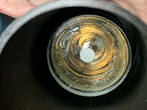
Figure 1: Geiger and Rutherford with their apparatus in 1912. Note autographs. For this setup,
Geiger himself was part of the detector: he visually counted flashes of light in the scintillator.

2    Description of Experimental Apparatus

Figure 2 is a simplified cross section of the scattering geometry located in the vacuum system. The
α-particle source is a circular foil of 5mm diameter plated with 241 Am, and the detector is a 9mm
diameter circle of ZnS powder located on the face of a 8575 photomultiplier. The scattering foil is
an annulus located coaxially with the α-source and detector with inner and outer diameters, 46.0
and 56.7 mm respectively. The angle β is determined by a fixed distance from source to scattering
foil. The scattering angle θ is varied by changing the distance from the scattering plane to the plane
of the detector. The metal stop prevents the direct beam of α-particles from striking the detector;
however, it can be removed to perform intensity and range measurements.

Figures 3 and 4 show the cage prepared for calibration and for a data run.

A scintillation counter is used to detect the α-particle. In this type of counter the detecting area is
covered with a thin coating of zinc sulfide activated by silver doping. When an α-particle strikes a
crystal of zinc sulfide, it emits a flash of light. The number of light quanta emitted is approximately
proportional to the energy lost by the α-particles in the crystal. If the initial energies of all the
α-particle were the same, the number of light quanta emitted for each incident α-particle would be
nearly constant. However, small variations in the kinetic energy of the α-particles, variations in the
efficiency with which the emitted light is converted into electrical signals by the PMT and variations
in the energy of the α-particles lost in the ZnS crystals give rise to a fairly broad distribution in the
size of the pulses from the detector. Figure 5 shows the arrangement of the ZnS scintillator on the
face of the PMT.

The blue light quanta emitted from the ZnS impinge upon the cathode of the photomultiplier and
electrons are emitted (the photoelectric effect). The number of electrons emitted by this process is

                                                   2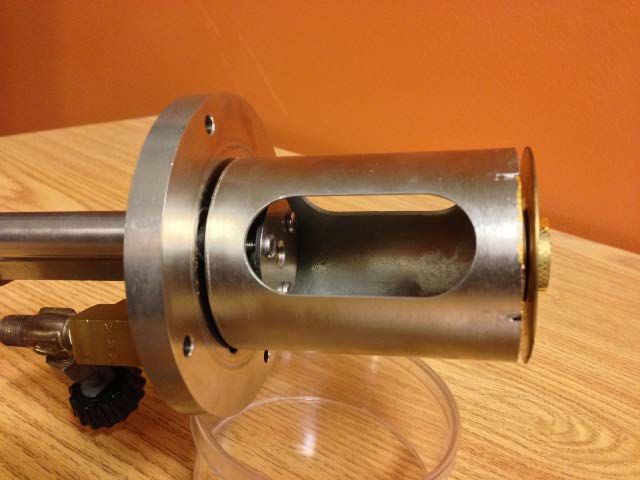
Figure 2: The apparatus. Note the four o-ring vacuum seals. The cylindrical scattering cage can
move over a range of about 20 cm from the detector by pushing the shaft (there are stops on the
end of the shaft which prevent hitting the detector even with the central plug inserted in the hole in
the middle of the scattering foil.) There is a brass shield and plug assembly which can be inserted
in front of the scattering foil for calibration. This entire assembly mounts vertically.

Figure 3: This image shows the cage with alpha source and gold scattering foil. Here the brass
shield and plug assembly (including washer for spacing away from the gold foil) has been inserted
in front of the scattering foil for calibration. The plug has a hole in the middle to form a direct
alpha beam, and this can be covered with gold foil to fully simulate the energy loss in the gold foil
scattering experiment.

                                                  3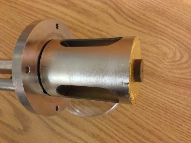
Figure 4: This image shows the cage with alpha source and gold scattering foil prepared for a
scattering run. Here only a central plug (without hole) has been inserted.

Figure 5: This image shows the ZnS scintillator placed in the middle of the face of the photomulti-
plier tube with optical grease.

                                                4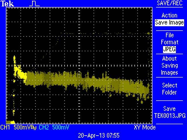
Figure 6: Block diagram of the detector and initial electronics chain. In this experiment you have
available two types of pulse-height analyzers (PHA): a multi-channel analyzer (MCA) which can
display the full spectrum with 1024 pulse height channels, and a 2-threshold single channel ana-
lyzer (SCA) and counter. Using the full spectrum of pulse heights displayed by the MCA, you can
decide where to set your SCA thresholds.

not sufficient for direct electronic detection so that they are first put through an electron multiplier
mounted within the tube itself. In the multiplier the process of secondary emission is used to
generate a cascade of electrons which increases from electrode to electrode. The photoelectrons
are accelerated to a dynode maintained at a higher potential than the cathode. The dynode emits
three or four times as many electrons as are incident on it, and the emitted electrons are accelerated
to the next dynode. This process is repeated 12 times, whereupon an amplification of from 10,000
to ten million is achieved (depending upon the voltage between dynodes). Since the number of
electrons emitted in the original photoelectric process depends upon the number of incident light
quanta, the number of electrons collected at the final anode of the phototube will be proportional
to the amount of scintillation light collected. The scintillation light is emitted by the zinc sulfide
crystal in about 10−4 seconds. The transit time of an electron cascade through the multiplier is less
than 10−7 seconds. A pulse of current may therefore be observed at the output of the phototube
for each α-particle incident upon the zinc sulfide, although the α-particles may arrive in rapid
succession. This pulse has a fast leading edge, and then a long trail lasting many microseconds.
Thus, you want to filter the pulse and count it within about 1 microsecond, avoiding pulse pileup.

The pulse of current from the photomultiplier charges a capacitor at the input to the preamplifier.
The amplifier further increases the size of the pulse and modifies its shape, so that it may be de-
tected and counted by the counter. The proper settings of the amplifier and of the high voltage
meter for the phototube will be given in the laboratory. They must be chosen so as to give adequate
amplification, but not so much that the pulses are too large for the amplifier to handle properly. As
mentioned above, the trapezoidal pulse out of the PMT must be smoothed and then differentiated,
yielding a more Gaussian shape of width about 1 microsecond. A pulse forming amplifier is avail-
able for that purpose. By adjusting PMT HV and amplifier gains, make sure most pulses are less
than 1V peak, and thus unsaturated.

In any electronic circuit electrical ”noise” (unwanted signals) is always present due to the random
motions of the electrons in the circuit. In this particular circuit a more important source of noise is
the thermionic emission of electrons from the photocathode which gives rise to signals at the anode
that look like small scintillation pulses. A discriminator is used at the input to the counter (as well
as the input to the MCA) to prevent these unwanted signals from being counted. The variable

                                                   5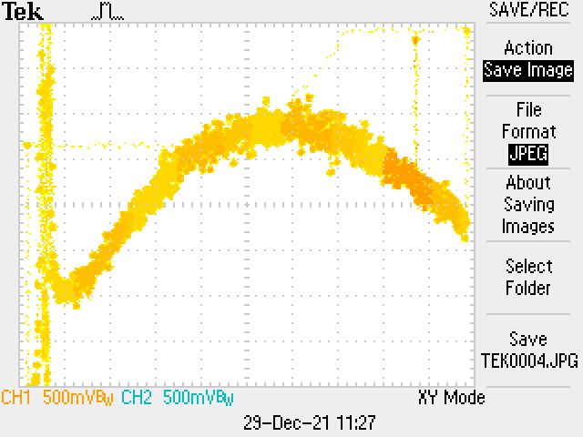
potentiometer on the discriminator controls this minimum voltage. In addition, and completely
separately from the MCA, you must choose a range of pulse heights (alpha energies) to integrate
over, and then count. This is done with the SCA which has upper, lower, and window mode
discriminators with a range of 0-10V. Its output can be sent to the counter. After some calibration,
you can easily know where to set the SCA window by referring to the 1024 channel MCA spectrum
displayed on the XY scope. The block diagram of the front end of the system (up to the pulse height
analysis) is shown in Figure 6.

Figure 7: Here the alpha beam was sent direct to the scintillator through a 2.3mm central hole in
the plug covered with gold foil. The Timing Filter Amplifier gain was 20. The output of the MCA
shows the full spectrum of pulse heights, 0-1V (and thus the spectrum vs alpha particle energy).
Little of the PMT noise is seen (note the discriminator on the MCA was set to reject pulses less than
about 100mV), and in the middle is the spectrum due to detected alphas. There is a broad peak,
and the integral counts over a window covering most of this alpha peak should be obtained for
each scattering angle. Although the XY output from the MCA has a 0-5V scale for display (hence
500mV per division on XY scope), the full range of pulse heights displayed is 0-1V so each division
of the X-axis corresponds to 0.1 V pulse height. The number of counts in each of the 1024 X-bins is
displayed on the Y-axis, with full range set by the full scale knob on the MCA.

If the pulses were all approximately of the same amplitude, the counting rate would be constant
over a range of discriminator settings. When the discriminator lower threshold is set too low the
counting rate will increase rapidly because of the PMT noise. If the discriminator is set too high,
most of the desired pulses will not be counted. In practice, the desired pulses have a range of sizes
so that no narrow peak can be found. However, a range of settings can be found where the counting
rate changes only slowly with discriminator setting, and the proper position for the discriminator
upper limit during the experiment is at the high counting rate end of the broad peak, (see Figure 7).
Obviously a discriminator lower threshold of 0.15V would encounter PMT noise background. The
full range of the MCA display 0-5V Y-axis corresponds to the COUNTS FULL SCALE range of the
Lecroy 3001 MCA setting knob, in 8 settings from 512 counts per pulse peak amplitude bin, up to
64K counts.

                                                 6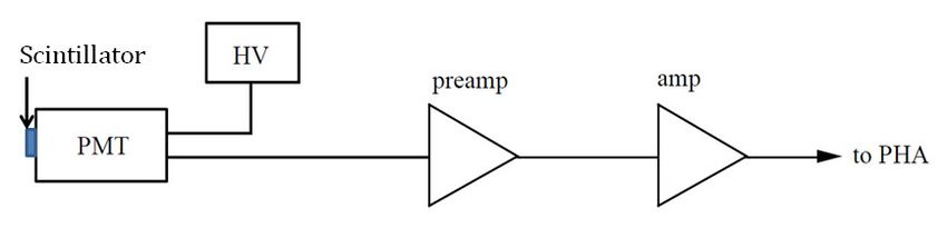
Care must be taken not to set the lower discriminator threshold too low, since the background from
the PMT can easily overwhelm the signal. Choose a level where the signal/background ratio is more
than 5 with the source maximally separated from the scintillator. With this setting almost all of the
desired pulses will be counted. The background spectrum can be taken with air in the system
and the source far away from the detector. At 1700V the PMT noise pulses [your background]
are usually less than 0.1V out of the preamp (200pF setting) with gain=20. Figure 8 shows the
Rutherford scattering spectrum with the cage pulled far from the detector.

Figure 8: The signal + background is shown using log scale on MCA for the source at its maximum
distance from the detector. The output of the MCA shows the full spectrum of the alpha signal at
this distance. To set up your filter amplifier window and counter, the dilemma is where to put the
lower window threshold: avoiding background by too high a threshold misses much of the alpha
signal; too low, and you are swamped by background. In this run, the PMT noise background can
be seen as the highlighted upturn at less than 0.2V. The count rate for a 0.3-0.9 volt interval was
0.06 counts per second.

3     Precautions

    1. Always turn off the high voltage before releasing vacuum and exposing the photomultiplier
       to room light. Exposure to even low levels of room light will destroy these photomultipliers
       which are very expensive.
    2. Do not open the vacuum system to air without consulting your instructor.
    3. Treat the scattering foil and mounting with care to avoid breaking the delicate foil.
    4. Do not touch the 241 Am source with anything.

Come to the laboratory with a brief outline of the experiment you intend to perform. You may
assume that the following quantities are known:

                                                   7
1 2
• 2 mv = 4.7 MeV = the energy of the α-particle (after traversing source window).
• Ze = 79e = total nuclear charge of each scattering atom
• ze = 2e = the charge of the α-particle
The thickness of a single foil is approximately 1 micron or 10−6 meter. You will use two layers.
The 5mm diameter 241 Am source is covered with a thin 1 micron gold-palladium foil to prevent
escape of radioactive daughter products and fragments of the source itself due to embrittlement.
The foil on the source reduces the α-particle energy from 5.48 MeV to the 4.7 MeV listed above. α-
particles traversing the gold foil in your scattering experiment will lose an additional 1 MeV. There
is some additional loss in the ZnS. These losses and other detector inefficiencies give rise to a tail
to lower energies seen in the MCA spectrum.
4 Relation between the differential cross section and the expected
counting rate
The differential scattering cross section is defined as
dσ # of particles scattered at angle θ into dΩ per unit time per target particle
=
dΩ # of particles incident per unit area per unit time (incident flux)
where θ is the polar angle, ϕ is the azimuthal angle, and the element of solid angle is dΩ =
d(cos θ)dϕ.
The total scattering cross section is Z
dσ
σ= dΩ.
dΩ
Note that the dimension of σ is area.
From the literature
Z 2 z 2 e4
θ
σ(θ) = csc4
16E 2 2
where:
Ze = the charge of the scattering center,
ze = the charge of the incident particle
E = the kinetic energy of the incident particle
and θ = the angle between the incident and scattered beams.
The coefficient of csc4 (θ/2) should be calculated before the experiment.
8Figure 9: The scattering geometry in this experiment, and definition of parameters. For your
setup, X is fixed. You will have to calculate Y from measurements of the extension of the rod. You
should make accurate measurements of the geometry of your system. This is the so-called Chadwick
geometry, which has a much higher collection efficiency than a conventional planar geometry where
the detector only intercepts a small fraction of the available solid angle at a given θ.
5 PRE-LAB basics
As shown in Figure 2, the scattering angle in this experiment is adjustable by moving the source-foil
assembly (cage) closer to the detector. You should make accurate measurements of the geometry
of your system. See Figure 9.
Some definitions:
∆Ω1 is the average solid angle subtended by the gold annulus at the source.
∆Ω2 is the average solid angle subtended by the detector at the scatterer.
(∆Ω2 = dΩ above in the definition of σ(θ).) Approximately :
A1 cos θ1
∆Ω1 ≈
R12
A2 cos θ2
∆Ω2 ≈
R22
(Check to see how good this approximation is for various angles.)
With the following definitions:
9N0 = the total number of particles emitted by the source per unit solid angle per unit time
A2 = the area of the detector
A1 = the area of the scattering material (gold foil)
ρ = the density of the scattering material
t = the thickness of the scattering material
L = Avogadro’s number
AG = the atomic weight of scattering material
n = ρLA1 t/AG = the total number of scattering centers
N1 = the total number of particles reaching A1 per unit time = N0 ∆Ω1 .
The incident flux is given by
N1 N0 ∆Ω1 N0
= ∼ 2
A1 cos θ1 A1 cos θ1 R1
N2 = total number of particles reaching A2 ; per unit time (expected rate):
nN0 nN0 A2 cos θ2
N2 = (incidentf lux) × σ(θ)∆Ω2 = 2 σ(θ)∆Ω2 = σ(θ)
R1 R12 R22
θ2 = θ − θ1 , θ = θ2 + θ 1
r0
R2 =
sin θ2
nN0 A2 cos θ2 sin2 θ2
Expected rate = σ(θ) = N2
R21 r20
The easiest parameter to measure for different values of the angle θ is the perpendicular distance
between the gold annulus and the detector. Let it be y.
y = R2 cos θ2 = r0 cot θ2
nN0 A2 Z 2 z 2 e4 cot θ2 sin3 θ2
N2 =
R12 r02 16E 2 sin4 (θ/2)
= N0 G f (y)
6 PRE-LAB
1. Using the values of the parameters given in the notes, estimate G, assuming t = 2 × 10⁻⁴ cm
(thickness of 2 gold foils); ρ = 19.32 g/cm3 ; fixed distance in Figure 1 = 6.75 cm; Eavg = 2.5
MeV (why so low?). WARNING: This step alone may take you several hours.
102. f (y) should be plotted versus y before the experiment. You will learn something that will
inform how you space your data runs in y.
3. Having found G, estimate what N0 should be for this experiment to give maximum precision
(2%) in a reasonable length of time. Remember you will need many points to establish the
angular distribution. The curve f (y) vs. y will give you an idea of how to space your points.
4. Think about how you are going to measure N0 . You are provided with a brass shield that
blocks α-particles scattered from the gold annulus, and a brass plug and washer. There is a
hole in the center of this plug, 2.3 mm (check this) in diameter, which allows an unscattered
beam to impinge on the detector.
5. What are the possible sources of systematic error? What experiments might you do to reveal
systematic error? You will document these tests in your lab report.
7 Procedure
The signal processing, pulse height range selection, and MCA electronics is shown in Figure 10.
1. First you must get detected pulses and then adjust the timing circuitry to give a clean unipolar
pulse of 1 microsec time constant approximately. Start with an intense beam of alphas using
a plug with an approx 1mm hole (no foil). After adjusting the HV, follow the pulse through
the system using the oscilloscope. There will be two amplitude families of pulses: low level
background and the higher level alphas. Make sure the alpha pulses are not saturated and
are the correct amplitude for insertion into the filter amplifier and the MCA. Repeat this for 2
layers of gold foil covering the hole (why?). Check the pulses out of the filter amplifier. Aim
for 0-1V.
2. You should have a scattering run generating a pulse height distribution (MCA output). A
plateau should be present (see Figure 8). It is suggested that the metal plug with a hole
covered with gold foil be first used to view the alpha energy distribution. The height of the
voltage pulse is a function of the energy and the lower voltage threshold of the filter amplifier
should be adjusted so as to count those α-particles which have lost considerable energy by
traversing the gold foil and still discriminate against noise.
3. You must determine the relationship between the measured rod extension and the internal
foil-detector distance y. You can make measurements when the system is apart. Be careful
not to touch the PMT face or detector with a ruler, and do not shine light on the PMT even
when it is off (scintillation lasts for days). Instead, for that measurement use our value of
the distance between the bottom of the vacuum flange (system open) and the bottom of the
flange at the PMT: 27.7 cm. See apparatus drawing. To this you should add 1.5mm for the
distance from the bottom of the PMT flange to the detector.
4. The dependence of the differential cross section on θ (the scattering angle) can now be found
by adjusting the relative position of the scattering foil with respect to the detector. You should
11plot the expected shape of the intensity vs. y (the perpendicular distance from the scintillator
to the plane of the gold foil) assuming Rutherford scattering to be valid. It is suggested that
in the laboratory you select ∼ 8 positions covering the entire range of y. Note that you do
not want to distribute the points uniformly in y (why?). For best results, you should integrate
over 2000 counts (∼2% statistical precision) in your optimal pulse height window for each
position of the foil relative to the detector. A goal might be 4000 counts, for better precision.
5. You will find it necessary to carefully plan your runs to take advantage of the lab time and
access. Overnight runs at each y will be necessary. If time permits, irregularities in the plot
of intensity vs. y can be investigated. Note that at low y scattering angles over 90 deg can be
obtained. Your integration time for a given statistical precision will be longer at y at 1 cm.
6. The strength of the source should be determined, using the brass blocking plate together with
the center plug with small hole. A gold foil covering this hole would assure the same energy
loss as in the main experiment. Backgrounds must be measured and subtracted from the data
before analysis. Plan how you will measure the various backgrounds (PMT, alphas scattering
off the inner metal walls ...). Recall that alphas have a short range in air. There is a plastic
sheet liner in the tube, so that alphas scatter off it rather than brass (why is this a good idea?).
8 Precautions and Directions on Rutherford Scattering experiment
1. PMT high voltage OFF when opening phototube to light.(Also keep fluorescent light away from
phototube). You may wish to turn the room fluorescent lights off while the can is out and the
tube is open. Use only incandescent lights.
2. Do not exceed 1900V. Raise HV slowly from zero. PMTs are noisy for hours after being turned
on.
3. Keep fingers off 241 Am source.
4. Treat gold foil with care:
• Put plug in from top of can.
• Caution inserting the can into the tube and its plastic sheet sleeve. Move the plastic
sleeve down so you can see it and carefully insert the can in the plastic.
• With can pushed up next to the detector (far away from the air rushing in) let air in
slowly (and then turn off pump). Observe this procedure when pumping down, too.
5. Don’t touch face of phototube with anything.
• Keep rulers, etc., away from the tube.
• Make sure plug will not hit the tube.
6. Keep away from the following hot spots.
• H.V. Supply
• Internal part of phototube box
129 Tests for Proper Operation
1. Make sure pulse never saturates anywhere in the analog signal chain.
2. Letting air in (slowly) should stop counts.
3. Raising H.V. a little should not increase nor decrease counting rate.
4. Raising window upper threshold should not decrease counting rate.
5. Decreasing PMT H.V. slowly to zero volts should stop counting rate.
There are other reactions taking place, that we ignore: Cherenkov radiation, bremsstrahlung and
inelastic nuclear interactions. See J.R. Comfort, et al., “Energy Loss and Straggling of α Particles in
Metal Foils,” Phys. Rev. 150, 249 (1966). This article includes data for gold foils.
Equipment supplied
• Vacuum pump
• Rutherford scattering assembly
• Am-241 100 micro Curie alpha source
• ZnS(Ag) scintillator alpha detector
• Burle 8575 12-stage PMT and negative HV base assembly
• Ortec 456 HV supply (operate around 1800V)
• Ortec 113 preamplifier (200pF gain setting)
• Ortek 474 filter amplifier. Start at gain = 20, integ=500ns, diff=200ns, inverted mode.
• LeCroy 3001 1K channel MCA V input mode, internal trigger
• Tektronix TDS 2022B X-Y scope for MCA pulse height spectrum display
• Ortec 550 SCA dual adjustable threshold amplifier
• Ortec 772 counter
• Tektronix DPO 3054 scope for pulse shape and timing tests
10 References
1. J. Earl, Modified Version of the MIT Rutherford Apparatus for Use in Advanced Undergraduate Laboratories,
Amer. J. Physics 34, 483 (1966).
2. R. D. Evans, The Atomic Nucleus, McGraw Hill (1972).
3. E. Rutherford, The Scattering of α and β-Particles by Matter and the Structure of the Atom, Phil.
Mag. 21, 669 (1911).
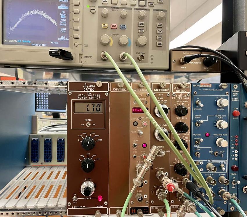
13Figure 10: The high voltage supply, signal processing (Timing Filter Amplifier) feeding the MCA
and SCA, SCA pulse height range selection, and MCA. The XY output of the MCA shows the full
spectrum of the alpha signal. To set up your filter amplifier window and counter, you must choose
where to put the SCA lower and upper window thresholds by reference to the MCA plot. Shown
is the result of an α beam integration of 19 hours at y=15cm, gain of 20, 0.3 - 0.9 V SCA range,
337,000 counts, and MCA range 1K full scale. The MCA input range is 0-1V, and the 1K channel
MCA memory is shown on the XY scope display (upper left) as a 0-5V signal in X and Y. The 0.3V
lower limit on the SCA corresponds to 3 of the 10 X-divisions on the scope.
14You can also read