The Milky Way tomography with APOGEE: intrinsic density distribution and structure of mono-abundance populations
←
→
Page content transcription
If your browser does not render page correctly, please read the page content below
Mon. Not. R. Astron. Soc. 000, 000–000 (0000)      Printed 25 April 2022    (MN LATEX style file v2.2)

                                               The Milky Way tomography with APOGEE: intrinsic
                                               density distribution and structure of mono-abundance
                                               populations
arXiv:2204.10327v1 [astro-ph.GA] 21 Apr 2022

                                               Jianhui Lian1,2? , Gail Zasowski2 , Ted Mackereth3 , Julie Imig4 , Jon A. Holtzman4 ,
                                               Rachael L. Beaton5,6 , Jonathan C. Bird7 , Katia Cunha8,9 , José G. Fernández-Trincado10 ,
                                               Danny Horta11 , Richard R. Lane12 , Karen Masters13 , Christian Nitschelm14 ,
                                               A.
                                               1
                                                  Roman-Lopes15
                                                 Max Planck Institute for Astronomy, 69117, Heidelberg, Germany
                                               2 Department   of Physics & Astronomy, University of Utah, Salt Lake City, UT 84112, USA
                                               3 Dunlap Institute for Astronomy and Astrophysics, University of Toronto, Toronto, Canada
                                               4 Department of Astronomy, New Mexico State University, Las Cruces, NM 88003, USA
                                               5 The Observatories of the Carnegie Institution for Science, 813 Santa Barbara Street, Pasadena, CA 91101, USA
                                               6 Department of Astrophysical Sciences, Princeton University, 4 Ivy Lane, Princeton, NJ, 08544, USA
                                               7 Department of Physics and Astronomy, Vanderbilt University, 6301 Stevenson Center, Nashville, TN 37235, USA
                                               8 Steward Observatory, The University of Arizona, Tucson, AZ, 85719, USA
                                               9 Observatório Nacional, 20921-400 So Cristóvao, Rio de Janeiro, RJ, Brazil
                                               10 Instituto de Astronomı́a, Universidad Católica del Norte, Av. Angamos 0610, Antofagasta, Chile
                                               11 Astrophysics Research Institute, Brownlow Hill, Liverpool, L3 5RF, UK
                                               12 Instituto de Astrofısica, Pontificia Universidad Católica de Chile, Av. Vicuna Mackenna 4860, 782-0436 Macul, Santiago, Chile
                                               13 Departments of Physics and Astronomy, Haverford College, 370 Lancaster Avenue, Haverford, PA 19041, USA
                                               14 Centro de Astronomı́a (CITEVA), Universidad de Antofagasta, Avenida Angamos 601, Antofagasta 1270300, Chile
                                               15 Departamento de Astronomı́a, Universidad La Serena, La Serena, Chile

                                               25 April 2022

                                                                                ABSTRACT
                                                                                The spatial distribution of mono-abundance populations (MAPs, selected in [Fe/H]
                                                                                and [Mg/Fe]) reflect the chemical and structural evolution in a galaxy and impose
                                                                                strong constraints on galaxy formation models. In this paper, we use APOGEE data
                                                                                to derive the intrinsic density distribution of MAPs in the Milky Way, after carefully
                                                                                considering the survey selection function. We find that a single exponential profile is
                                                                                not a sufficient description of the Milky Way’s disc. Both the individual MAPs and
                                                                                the integrated disc exhibit a broken radial density distribution; densities are relatively
                                                                                constant with radius in the inner Galaxy and rapidly decrease beyond the break ra-
                                                                                dius. We fit the intrinsic density distribution as a function of radius and vertical height
                                                                                with a 2D density model that considers both a broken radial profile and radial vari-
                                                                                ation of scale height (i.e., flaring). There is a large variety of structural parameters
                                                                                between different MAPs, indicative of strong structure evolution of the Milky Way.
                                                                                One surprising result is that high-α MAPs show the strongest flaring. The young,
                                                                                solar-abundance MAPs present the shortest scale height and least flaring, suggesting
                                                                                recent and ongoing star formation confined to the disc plane. Finally we derive the
                                                                                intrinsic density distribution and corresponding structural parameters of the chemi-
                                                                                cally defined thin and thick discs. The chemical thick and thin discs have local surface
                                                                                mass densities of 5.62±0.08 and 15.69±0.32 M pc−2 , respectively, suggesting a mas-
                                                                                sive thick disc with a local surface mass density ratio between thick to thin disc of
                                                                                36%.
                                                                                Key words: Galaxy: structure – Galaxy: disc – Galaxy: abundances – Galaxy: stellar
                                                                                content – Galaxy: fundamental parameters – Galaxy: evolution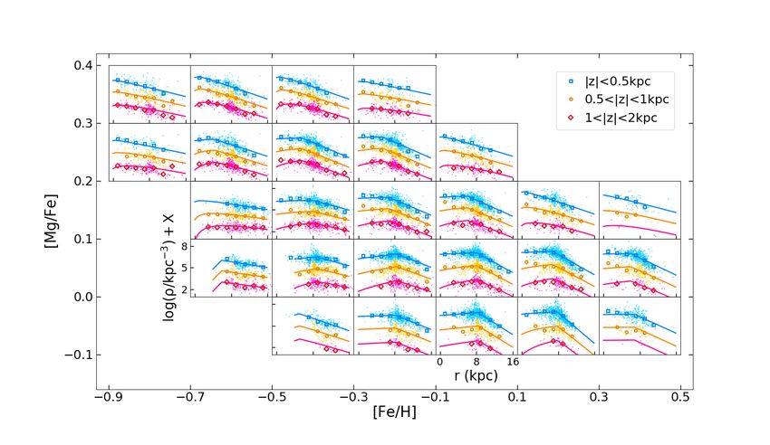
2     J. Lian et al.
1   INTRODUCTION                                                   comparable scale length between the thick and thin disc in
                                                                   external galaxies (Comerón et al. 2012).
The stellar structure of the Milky Way, along with the chem-             In addition to the geometric dichotomy, many works
ical and kinematic configurations, place critical constraints      have also identified a dichotomy in chemical compositions of
on models of our Galaxy’s formation and evolution. Our po-         stars in the solar neighborhood with two well separated se-
sition at the Solar circle with a small vertical distance from     quences in [α/Fe]-[Fe/H] distribution (e.g., Fuhrmann 1998;
the disc plane allows us to study the Galactic disc struc-         Reddy et al. 2006; Lee et al. 2011; Adibekyan et al. 2012;
ture in great detail on a star by star basis. The disc of the      Haywood et al. 2013; Bensby et al. 2014; Hayden et al. 2015).
Milky Way is generally thin, providing us a relatively un-         This geometric and chemical dichotomy in disc stars are
obscured view in the vertical direction into the stellar halo      not identical, but they share significant overlap. While some
but highly obscured view in the disc plane, especially at the      chemical thin disc stars may be found in the geometric thick
Galactic center direction. As a consequence, the local sur-        disc, it is characterized by old, α-enhanced, and kinemati-
face density and vertical density profile have been robustly       cally hot populations, while the geometric thin disc mostly
measured (e.g., Gilmore & Reid 1983; Bienayme et al. 1987;         consist of younger, solar-α, and kinematically cooler pop-
Robin et al. 2003; Flynn et al. 2006; Jurić et al. 2008; McKee    ulations (e.g., Bensby et al. 2005; Lian et al. 2020b). This
et al. 2015), while the radial and vertical structure beyond       connection between the geometric and chemical dichotomy
the solar radius are more uncertain.                               implies close relation between the thick/thin disc structure
                                                                   formation and the chemical evolution history of the Galaxy
     An exponential form is commonly used to describe the          (Lian et al. 2020b; Horta et al. 2021).
radial and vertical density distribution of the Galactic and
                                                                         A variety of scenarios have been suggested to explain
extragalactic disc (e.g., Freeman 1970; Gilmore & Reid 1983;
                                                                   the chemical dichotomy and its implication for thick/thin
Robin et al. 2003; Pohlen & Trujillo 2006). Early studies of
                                                                   disc formation. One of them attributes the formation of
the Galaxy structure is generally based on stellar photomet-
                                                                   metal-poor, low-α populations to a recent gas accretion and
ric observations without distance information (e.g., Bahcall
                                                                   star burst event (Calura & Menci 2009; Haywood et al. 2019;
& Soneira 1980). The derived structure parameters by fit-
                                                                   Spitoni et al. 2019; Buck 2020; Lian et al. 2020a,b; Agertz
ting simple models to the projected star counts usually suffer
                                                                   et al. 2021). In this scenario, the thick and thin discs are es-
large uncertainties due to degeneracy between different pa-
                                                                   tablished locally and successively. In contrast, another sce-
rameters. While the scale length of external galaxies are well
                                                                   nario assumes the high- and low-α sequences formed in par-
established (e.g., Fathi et al. 2010; Lange et al. 2015), a wide
                                                                   allel but at different locations in the Galaxy and mixed up
range of values from 1.8 to 6.0 kpc have been reported for the
                                                                   later on via radial migration (Grisoni et al. 2017; Mackereth
Milky Way’s disc in the literature (see Bland-Hawthorn &
                                                                   et al. 2018). The mixing through radial migration is also
Gerhard 2016 for a review). Comparing to external galaxies
                                                                   required in another explanation that adopts a continuously
at similar stellar masses, the scale length of Milky Way’s disc
                                                                   varying star formation history with radius (Chiappini 2009;
seems systematically shorter (Licquia et al. 2016; Boardman
                                                                   Minchev et al. 2015; Andrews et al. 2017; Sharma et al. 2020;
et al. 2020). This suggests the Milky Way might be an unusu-
                                                                   Johnson et al. 2021). In addition, clumpy star formation is
ally compact galaxy for its mass, or there are inconsistences
                                                                   also suggested to be capable of generating the chemical di-
between the methods used for scale length measurements in
                                                                   chotomy (Clarke et al. 2019).
the Milky Way and other galaxies.
                                                                         Recently, with chemical observations being available be-
     Star counts in the vertical direction in early studies re-    yond the solar neighborhood, many works have confirmed
vealed that the Milky Way’s disc consists of two components        the nearly invariant locus of high-α sequence, which is usu-
with distinct thickness, which are commonly referred to as         ally referred to as ‘chemical thick disc’, in [α/Fe]-[Fe/H] dis-
the geometric ‘thick’ and ‘thin’ discs (Yoshii 1982; Gilmore       tribution across the Galaxy (e.g., Weinberg et al. 2019; Katz
& Reid 1983; Robin et al. 2003; Jurić et al. 2008). After         et al. 2021). This suggests highly homogeneous chemical en-
being discovered in external galaxies by Burstein (1979),          richment in the early times or thoroughly mixing after the
such geometric thick/thin disc dichotomy was found to be           establishment of high-α disc. The characteristics of geomet-
common in local disc galaxies (Yoachim & Dalcanton 2006;           ric thick disc, however, changes from the inner to the outer
Comerón et al. 2012). Gilmore & Reid (1983) provided the          disc, where the region high above the disc is increasingly
first reliable vertical stellar density distribution and esti-     dominated by intermediate age, metal-poor, low-α popula-
mated a scale height (hZ ) of 1350 pc for the thick disc and       tions (Nidever et al. 2014; Hayden et al. 2015; Queiroz et al.
300 pc for the thin disc. Similar values are suggested in Siegel   2020). This results in a radial age gradient in the geometric
et al. (2002) using improved photometric data from wide-           thick disc (Martig et al. 2016b). This finding complicates
field CCDs. With a large sample of M dwarfs in SDSS pho-           the formation picture of Milky Way’s disc and illustrate the
tometry survey, Jurić et al. (2008) obtained a hZ of 300 pc       importance of studying the Galaxy beyond the solar vicin-
for the thin disc in good agreement with previous works,           ity to draw a comprehensive picture of the formation and
and 900 pc for the thick disc lower than earlier estimates.        evolution of the Milky Way.
Unlike the scale height at solar radius, the scale length (hR )          The advent of massive stellar spectrosopic surveys,
is more difficult to measure due to the high extinction on         which cover a large portion of the Galaxy, such as APOGEE
the disc plane. Jurić et al. (2008) reported a scale length of    (Majewski et al. 2017), GALAH (Martell et al. 2017), LAM-
the thin disc shorter than the thick disc (2.9 versus 3.6 kpc).    OST (Zhao et al. 2012), and Gaia-ESO (Gilmore et al. 2012),
However, an opposite result is found in Cheng et al. (2012)        have enabled the studies of spatial and chemical structure
with a scale length of 3.4 kpc for the thin disc and 1.8 kpc       beyond the solar radius. Taking advantage of the wide spa-
for the thick disc. Interestingly, deep imaging data reveals       tial coverage of these surveys, many works have explored the
Density distribution and structure of MAPs                   3
structure of mono-abundance/age populations which reflects              In §2, we illustrate the APOGEE data and age distribu-
the growth history of the Milky Way and provide critical in-       tion of MAPs that are used to calculate the selection func-
sights into mechanisms that drive the disc formation and           tion. The calculation of the APOGEE selection function is
evolution. Bovy et al. (2012b) studied the mono-abundance          then presented in the following §3. In §4 we present the
populations (MAPs; defined in [Fe/H] and [α/Fe] space) in          intrinsic density distribution of MAPs after correcting for
the Milky Way using a sample of G-dwarfs in SEGUE sur-             selection function, the density model, and the fitting results
vey. They found a radially compact, but vertically extended        of structure parameters for each MAP. In §5 we discuss the
morphology of high-α disc, and a continuous transforma-            potential systematics in the results and compare our mea-
tion from the thick high-α disc to the thin low-α disc in          surements with previous works. We also derive the density
spite of discontinuity in chemical abundance distribution.         distribution and measure the structure of the total stellar
Bovy et al. (2016b) extended this work to red-clump giants         populations in §5.3 to facilitate comparison with earlier pho-
in APOGEE survey and suggested a broken profile is needed          tometric works in the Milky Way and studies of external
to well fit the radial density distribution of the low-α disc.     galaxies. Finally, a summary of our results is included in §6.
The density model is also improved on the basis of Bovy
et al. (2012b) to consider possible radial variation of scale
height for each MAP. The authors found a constant thick-
                                                                   2     SAMPLE SELECTION
ness of high-α MAPs, but the scale height of low-α MAPs
increases with radius (i.e. flares). This broken radial profile    2.1    Selection criteria
and flaring of low-α disc is confirmed in Mackereth et al.
(2017) where the authors dissect the disc stars for the first      We select our stellar sample from APOGEE catalogue (all-
time into mono-age, mono-abundance populations. More re-           star summary file) contained in the last internal data re-
cently, Yu et al. (2021) studied the structure of MAPs using       lease after SDSS-IV Data Release 16 (DR16; Ahumada et al.
LAMOST data, and found a clear signature of flaring in             2020; Jönsson et al. 2020), which includes data from ob-
both high- and low-α MAPs. Many theoretical works have             servations until March 2020, reduced with a very slightly
also paid attention to the mono-abundance/age populations          updated version of the DR16 pipeline (r13). APOGEE is
in simulated galaxies to understand the observed structure         a near-infrared, high-resolution spectroscopic survey (Blan-
of MAPs in the Milky Way (e.g., Stinson et al. 2013; Bird          ton et al. 2017; Majewski et al. 2017) that primarily targets
et al. 2013; Minchev et al. 2015). Although facing many chal-      evolved giant stars in the Milky Way and Local Group satel-
lenges to match the high-dimensional observations in the           lites (Zasowski et al. 2013, 2017; Beaton et al. 2021; Santana
Milky Way, the mono-abundance/age populations of simu-             et al. 2021). This survey is performed using custom spectro-
lated galaxies have structure in qualitative agreement with        graphs (Wilson et al. 2019) with the 2.5 m Sloan Telescope
the Milky Way (e.g., Stinson et al. 2013; Bird et al. 2013;        and the NMSU 1 m Telescope at the Apache Point Obser-
Martig et al. 2014).                                               vatory (Gunn et al. 2006; Holtzman et al. 2010), and with
                                                                   the 2.5 m Irénée du Pont telescope at Las Campanas Ob-
     In this paper we investigate the structure of MAPs
                                                                   servatory (Bowen & Vaughan 1973).
in the Milky Way using the latest APOGEE observations
                                                                         The chemical abundances ([Fe/H], [Mg/Fe]) and stel-
which incorporates the data recently acquired at Las Cam-
                                                                   lar parameters (i.e., log(g) and Teff ) are taken from the
panas Observatory at south hemisphere and provide a better
                                                                   APOGEE catalogue which are derived by custom pipelines
coverage of the inner Galaxy. Most previous MAP studies
                                                                   ASPCAP described in Nidever et al. (2015), Garcı́a Pérez
have used a forward modelling approach which first predicts
                                                                   et al. (2016) and Holtzman et al. in prep and line list in
the number of stars at each Galactic location probed by the
                                                                   Smith et al. (2021).
survey by applying the survey selection function to a pre-
                                                                         We use the recommended stellar ages and spectro-
sumed Milky Way density model and then tune the model
                                                                   photometric distances in the astroNN Value Added Catalog
parameters to achieve a good match to the data (Bovy et al.
                                                                   for the internal data release (Mackereth et al. 2019)1 . The
2012b, 2016b; Mackereth et al. 2017). With this approach,
                                                                   ages are derived by training a deep neural network (Leung &
the intrinsic density distribution of MAPs are unknown until
                                                                   Bovy 2019a)2 with asteroseismic ages derived from Kepler
a good fit by the model is achieved. In this work we adopt
                                                                   and APOGEE combined observations (Pinsonneault et al.
a different method to first recover the spatial density dis-
                                                                   2018). We note that α-rich stars at [Fe/H]< −0.5 may be
tribution of the underlying intrinsic population, including
                                                                   subject to extra mixing (Shetrone et al. 2019) which would
stars not observed, for each MAP from observations after
                                                                   affect spectroscopic age determination but has not been con-
carefully accounting for the survey selection function. We
                                                                   sidered in the astroNN age measurement. Moreover, the
then fit a density model to the intrinsic, selection-function
                                                                   abundance space at [Fe/H]< −0.5, [Mg/Fe]> 0.2 is not well
corrected, density distribution to derive structural parame-
                                                                   populated by the training sample. Therefore, in this work we
ters of MAPs. In this way we can construct a more realistic
                                                                   only use the astroNN ages for high-α ([Mg/Fe]> 0.2) stars
and representative density model with the guidance from
                                                                   with [Fe/H]> −0.5. The distances in astroNN catalogue are
the intrinsic density distribution. Another advantage of this
                                                                   determined by training the neural network on stars in com-
method is that it is more straightforward to identify features
                                                                   mon between Gaia and APOGEE (Leung & Bovy 2019b).
in the density distribution that is not captured by the model
which possibly indicate substructures in the Galaxy. The re-
sult of this work also lay the foundation for future works         1 The Value Added Catalog for the public Data Release 16 is
to measure the global stellar population properties of the         available at https://data.sdss.org/sas/dr16/apogee/vac/apogee-
Milky Way, in a model-independent way, that allow direct           astronn
comparison with observational results of external galaxies.        2 https://github.com/henrysky/astroNN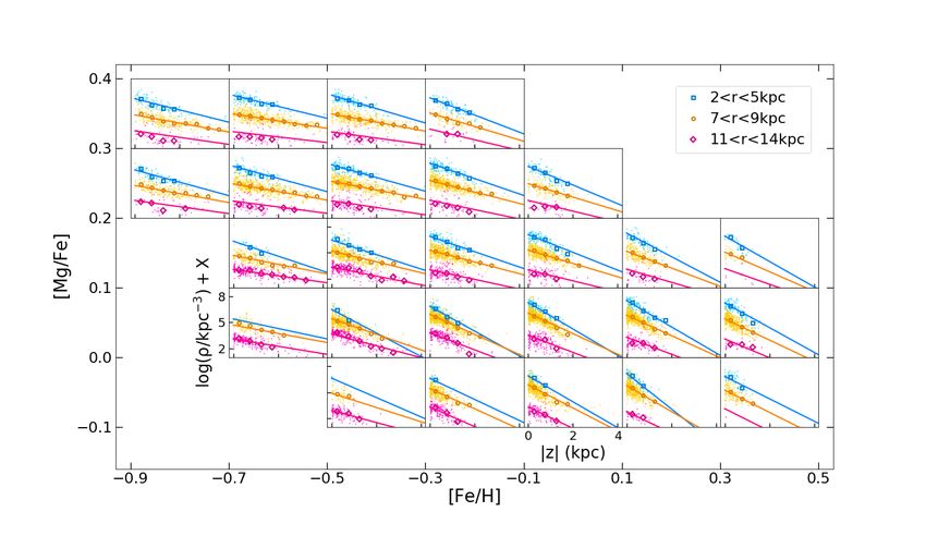
4     J. Lian et al.
    We use the following criteria to select a sample of stars     1997; Kobayashi et al. 2006; Lian et al. 2020b), the age
with reliable measurements from the parent APOGEE cat-            difference between stars in the high-α sequence should be
alogue:                                                           within 2 Gyr. We have tested that, at age older than 8 Gyr,
                                                                  changing the age by 2 Gyr results in only a 7% difference
 • Signal-to-Noise ratio (SNR) > 50,
                                                                  in the selected fraction of APOGEE targets. Therefore we
 • EXTRATARG== 0,
                                                                  conclude that the selection function of metal-poor, high-α
 • APOGEE TARGET1 and APOGEE2 TARGET1 bit 9
                                                                  mono-abundance bins derived from extrapolated age distri-
== 0,
                                                                  butions is robust.
EXTRATARG==0 identifies stars in the main survey, in                   It is interesting to note that the radial variation be-
which stars were randomly selected, and removes dupli-            havior in the age distribution is clearly different between
cated observations. The ninth bit of APOGEE TARGET1               MAPs (Figure 1). In the high-α mono-abundance bins
or APOGEE2 TARGET1 are set for targets that are pos-              ([Mg/Fe]>0.2), the age distribution at various radii are
sible star cluster members. For more details about the            rather similar, suggesting a spatially homogeneous chemi-
APOGEE bitmasks, we refer the reader to https://www.              cally defined thick disk at the present day. This is in line
sdss.org/dr16/algorithms/bitmasks/.                               with the nearly universal median locus of high-α sequence
      To study the structural evolution of our Galaxy that        in the [α/Fe]-[Fe/H] diagram (Nidever et al. 2014; Hayden
consists of sub-populations formed at different epochs with       et al. 2015; Weinberg et al. 2019; Katz et al. 2021). In con-
different chemical abundances, it is ideal to obtain the den-     trast, the age distributions of MAPs at low-α ([Mg/Fe] 0.2
     As we lack reliable age measurements at [Fe/H]< −0.5,        show little variation with height, while the low-α stars with
to calculate the selection function for high-α ([Mg/Fe]>0.2)      the same abundances tend to be older at larger vertical dis-
MAPs below this metallicity, we assume they have the same         tance. A possible origin of this vertical trend is secular disc
age distribution as the MAPs at the same [Mg/Fe] and              heating, possibly by the pre-existing thick disc or interac-
−0.5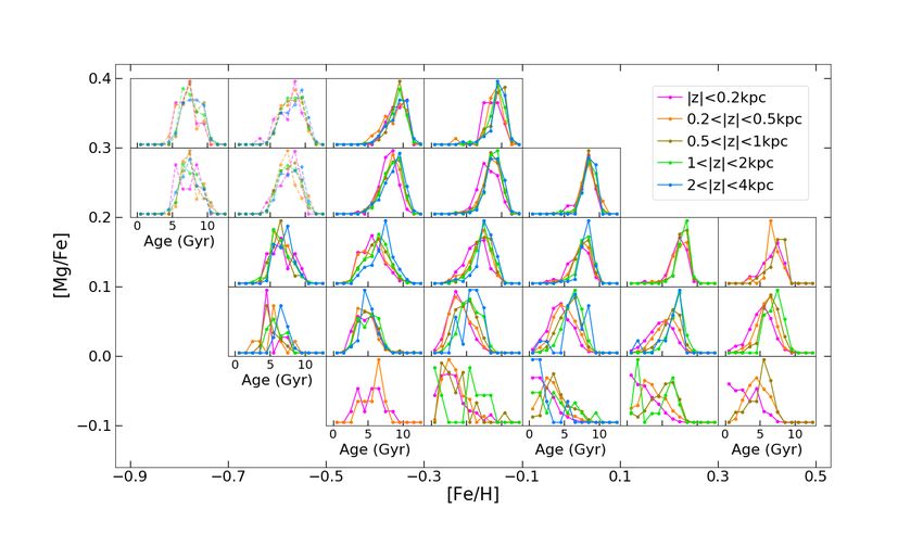
Density distribution and structure of MAPs                        5

Figure 1. Normalized age distribution of mono-abundance populations on the mid-plane (|Z| < 0.2 kpc) as a function of Galactocentric
radius. Since the age measurement at [Fe/H]< −0.5 is unreliable (see §2.1), for the four high-α mono-abundance bins at [Fe/H]< −0.5
we assume they have the same age distribution of mono-abundance populations with the same [Mg/Fe] and −0.5
6       J. Lian et al.
                                                                     (Bovy et al. 2016a) and a combined 3D dust map from Mar-
                                                                     shall et al. (2006), Green et al. (2019), and Drimmel et al.
                                                                     (2003) (see Bovy et al. 2016a for details on the combina-
                                                                     tion). The first component of APOGEE selection function,
                                                                     fCMD , is then calculated by applying the APOGEE target
                                                                     selection limits and counting the fraction of stars that falls
                                                                     within these limits.
                                                                          Figure 3 illustrates this fraction as a function of he-
                                                                     liocentric distance for a short cohort in a disk field (field
                                                                     ID: 2254) as an example. Each line indicates a single mono-
                                                                     abundance bin as denoted in the legend. Note that the MAPs
                                                                     in the legend from top to bottom have decreasing mean ages.
                                                                     It can be seen that fCMD generally decreases with increas-
                                                                     ing distance, mainly due to fainter apparent H magnitude.
                                                                     Three of the four mono-abundance bins have a similar fCMD ,
                                                                     while the youngest one ([Fe/H]=0, [Mg/Fe]=-0.05) shows
                                                                     lower fraction at the smallest distance but higher fraction
                                                                     at distance beyond 3 kpc. This different behavior at vari-
                                                                     ous distances is a result of two competing effects: younger
Figure 3. Fraction of the underlying stellar population satisfying   populations are brighter, which increases their fCMD , but at
APOGEE target candidates definition as a function of heliocen-       younger ages the red giant stage is populated by more mas-
tric distance for a short cohort in a APOGEE disc field (field ID:
                                                                     sive stars, which are rarer and spend less time in the RGB,
2544, l = −24.6°, and b = 46.5°). The fraction of mono-abundance
populations are calculated separately and four of them are shown
                                                                     resulting in a lower fCMD . At small distances, red giant stars
in four lines with different colour.                                 are generally bright enough to meet the target candidate se-
                                                                     lection limits and therefore the latter effect is dominant. In
                                                                     contrast, at larger distances, the brightness of stars become
3.1     Target candidates selection                                  more important and younger stars will have larger chance
                                                                     to be selected as targets. However this age effect is only sig-
The targets in the APOGEE main survey are selected from
                                                                     nificant at young ages when the age-luminosity relation is
candidates defined by (J − K)0 colour and H magnitude in
                                                                     relatively steep. Therefore the selected fraction of the three
2MASS Point Source Catalog (Skrutskie et al. 2006). For
                                                                     mono-abundance bins with intermediate and old ages do not
full details of the targeting strategy, we refer the reader
                                                                     show clear deviation from each other.
to Beaton et al. (2021) and Santana et al. (2021), but
we summarize the relevant information here. The dered-
dened (J − K)0 colour is derived using the Rayleigh-Jeans            3.2    Selection of spectroscopic target and final
Color Excess Method (Majewski et al. 2011) or extinction                    abundance sample
map from Schlegel et al. (1998). The range of (J − K)0
colour for target selection varies between fields. APOGEE-           APOGEE main survey targets are randomly drawn from the
1 and APOGEE-2 bulge fields use a single colour limit of             photometric candidates defined in (J − K)0 and H. The se-
(J − K)0 > 0.5, while APOGEE-2 halo fields adopt a bluer             lected fraction in this step, fspec , is a only function of field
cut with (J − K)0 > 0.3. To increase the fraction of dis-            and cohort, and also (J − K)0 colours in case of APOGEE-2
tant red giant stars, APOGEE-2 disc fields select targets            disc fields. The fspec for APOGEE DR16 is publicly avail-
separately from two colour bins; 0.5 6 (J − K)0 < 0.8 and            able5 (Bovy et al. 2014; Bovy 2016). We assume this fraction
(J − K)0 > 0.8. In each field, a group of stars with ex-             does not change from DR16 to the incremental post-DR16
actly the same visits are referred to as a ‘cohort’. For a sin-      release and adopt this fspec in this work.
gle field, there are a maximum of three cohorts, with three               In some unusual cases, such as abnormally low spectra
non-overlapping H magnitude ranges corresponding to three            quality/SNR, extreme stellar parameters close to or exceed-
different depth of observations. While the exact range of H          ing the edge of ASPCAP grid, a small fraction of targeted
magnitude used for target selection depends on the field and         stars do not have well-determined chemical compositions.
number of visits of the cohort, for reference, the typical H         These objects are excluded from the final stellar sample by
magnitude range for the most common ‘short’ cohort which             applying the selection criteria described in §2.1. For each
has the least number of visits is 7−12.2 mag.                        MAP in each field and cohort, we calculate the fraction
     For each MAP at each heliocentric distance in a given           of targeted stars meeting the selection criteria in §2.1 for
field and cohort, we use the galactic location-dependent age         reliable abundance measurements, fabun , which is the final
distribution and PARSEC evolution tracks3 (Bressan et al.            patch of the APOGEE effective selection function. Figure 4
2012) with bolometric corrections from Chen et al. (2019) to         illustrate the selection of targets and final stellar sample for
simulate the stellar distribution in the observed (J − K)0 -H        the same field and cohort in Fig. 3. The distribution of stars
CMD. We adopt a Kroupa IMF (Kroupa 2001) and calcu-                  in the 2MASS Point Source Catalogue in this field is shown
late extinction in H band using the python package mwdust4           in grey in the background. Selected targets are indicated as
                                                                     green dots, with fspec in the blue and red colour bins of 0.166

3   http://stev.oapd.inaf.it/cgi-bin/cmd
4   https://github.com/jobovy/mwdust                                 5   https://github.com/jobovy/apogee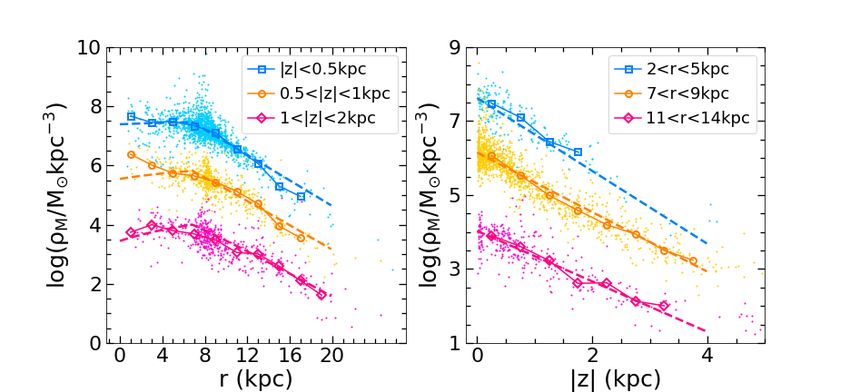
Density distribution and structure of MAPs                        7
                                                                       the fraction in the three selection steps as:
                                                                        feff ([Fe/H], [Mg/Fe], F, C,d) =
                                                                                                      fCMD ([Fe/H], [Mg/Fe], F, C, d)
                                                                                                       × fspec (F, C) × fabun (F, C)
                                                                                                                                       (1)
                                                                       for fields have target candidates selected on single J − K0
                                                                       colour bin, or
                                                                       feff ([Fe/H], [Mg/Fe], F, C, J − K0 , d) =
                                                                                                  fCMD ([Fe/H], [Mg/Fe], F, C, J − K0 , d)
                                                                                                   × fspec (F, C, J − K0 )
                                                                                                   × fabun (F, C, J − K0 )
                                                                                                                                       (2)
                                                                       for fields with target candidates selected in two colour bins
                                                                       separately. Here d stands for heliocentric distance, F and
                                                                       C stand for field and cohort, respectively. To calculate a
                                                                       consistent feff for all fields, in fields with targets selected in
                                                                       two colour bins, we further calculate an average feff weighted
Figure 4. APOGEE target selection in (J − Ks )0 − H for the
same field and cohort as Fig. 3. The distribution of stars in          by the number of stars in each colour bin as predicted by
2MASS Point Source Catalogue in this field is shown in the back-       the theoretical isochrones in §3.1. Note that, to calculate
ground in grey. Green dots are those that are selected for target-     the intrinsic number density, dividing the total number of
ing and the orange circles denote stars in the final stellar sample    stars observed in the two colour bins by the average selection
with robust abundance measurements. Dashed lines indicate the          fraction is equivalent to doing this calculation separately in
selection limits for target candidates in the CMD. For this field      each colour bin and then summing them up. For reference,
the target selection is performed in two colour bins separately to     feff for the low-α, metal-rich MAP of [Mg/Fe]=0.05 and
have a better coverage of distant stars.                               [Fe/H]=0.4 at a distance of 1 kpc in the short cohort of the
                                                                       field in Fig.4 are 6.30×10⁻⁴ and 3.06×10⁻³ in the blue and
                                                                       red colour bins, respectively.
                                                                            To give a global view of the APOGEE effective selec-
                                                                       tion function, we show in Figure 5 the X-Y distribution of
                                                                       feff of all cohorts in the Galactic plane (|Z| < 0.2 kpc). Each
                                                                       cohort is separated into 13 distance bins, from 0.5 to 20 kpc.
                                                                       The bin size is smaller for closer distances to ensure approx-
                                                                       imately even number of stars in each distance bin. A more
                                                                       detailed discussion on the number statistics is given in 6.1.
                                                                       The effective selection fraction is higher at smaller distance
                                                                       where stars are brighter, and lower in the Galactic center
                                                                       direction owing to higher stellar density and extinction to-
                                                                       wards the inner Galaxy.

                                                                       4     DENSITY DISTRIBUTION OF
                                                                             UNDERLYING MONO-ABUNDANCE
                                                                             POPULATIONS
                                                                       4.1    Spatial distribution of sampled underlying
                                                                              populations
                                                                       With the effective selection function, we can derive the num-
Figure 5. Distribution of effective selection fraction at various      ber density of underlying populations by simply dividing the
distances of all cohorts with |Z| < 0.2 kpc in X-Y plane.              observed density by the selected fraction:
                                                                                                      ρobs ([Fe/H], [Mg/Fe], F, C, d)
                                                                       ρint ([Fe/H], [Mg/Fe], F, C, d) =                               ,
                                                                                                       feff ([Fe/H], [Mg/Fe], F, C, d)
                                                                                                                                  (3)
                                                                       where ρobs indicates the observed number density, which
and 0.853, respectively. Stars in the final stellar sample are         equals the number of observed stars divided by the volume
shown in orange circles, which comprise 97.3% and 92.0% of             of each distance bin at a given field. The different fields of
the targeted sample in the blue and red colour bins, respec-           view on the telescopes at Apache Point Observatory and
tively. The effective selection fraction, feff , is a product of       Las Campanas Observatory have been taken into account.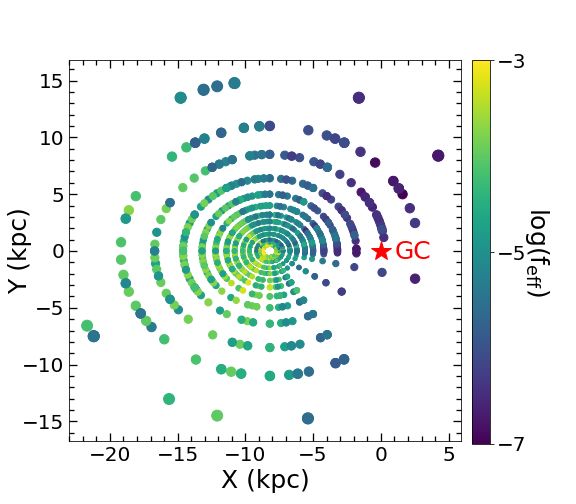
8     J. Lian et al.

Figure 6. Spatial distribution of intrinsic number density of four MAPs in the X-Y plane (with |Z| < 0.2 kpc) in the middle row and the
R-|Z| plane in the bottom row. Each symbol indicates one spatial bin, with the location determined by the average position of observed
stars in each bin. The symbol size of each bin is proportional to its heliocentric distance. Each column is for one MAP, with decreasing
mean age from the left to the right. The abundance range of each MAP is indicated by the orange box in the top row, on top of the
distribution of the whole APOGEE sample shown in grey contours.

The calculation of intrinsic number density is performed in-           compared to the high-α population. The similarity in ra-
dependently for each combination of [Fe/H], [Mg/Fe], and               dial extension supports the hypothesis of an evolutionary
distance in each field’s set of cohorts. To improve statistics,        connection between these two stellar popoulations. The dis-
we rebin all APOGEE fields with a semi-regular (l, b) grid             crepancy in vertical extension, combined with their distinct
with 2.7 fields in each grid element on average. For each spa-         chemical abundances (e.g., Hayden et al. 2015) and different
tial location (l, b, d), the average recovered intrinsic number        kinematic properties (e.g., Robin et al. 2017), however, sug-
density of all cohorts is used.                                        gests an upside-down disc formation with a transition from
     Figure 6 shows the spatial distribution of intrinsic num-         rapid assembly of a kinematically hot, thick disc to secular
ber density distribution of four MAPs in the X-Y plane (with           establishment of a kinematically cold, thin disc (Bird et al.
|Z| < 0.2 kpc) in the middle row and the R-|Z| plane in the            2013; Freudenburg et al. 2017). This transition is likely con-
bottom row. Each symbol indicates one spatial bin, with                nected to the early quenching process, possibly driven by
the location determined by the average position of observed            the same mechanism, which remains unclear.
stars within this bin. The symbol sizes are proportional to                  The metal-poor, low-α population (third column in
their distance to the Sun. Each column shows the distribu-             Fig. 6), which has an average age slightly younger than the
tion of a single MAP formed at different epochs of the Milky           metal-rich, low-α population, displays a very different spa-
Way’s evolutionary history, following an order of decreasing           tial distribution. It shows a clearly extended distribution in
mean age from the left to the right. In the top row, the po-           both radial and vertical direction. In particular, among the
sition of each MAP in [Mg/Fe]-[Fe/H] distribution is shown             four MAPs considered, this metal-poor, low-α MAP shows
as orange box, on top of the whole APOGEE sample shown                 the largest radial distribution, out to 20 kpc. This is in line
as grey contours.                                                      with the finding that the outer disc beyond 15 kpc is domi-
      It is interesting to note that stellar populations with          nated by metal-poor, low-α stars (Lian et al. 2022, Evans et
different abundances have noticeably different three dimen-            al. in prep). The large vertical extension of this population,
sional spatial distributions. The old, high-α populations              combined with its wide radial distribution, leave the metal-
(first column in Fig. 6) have relatively limited radial dis-           poor, low-α stars as the dominant population in the geomet-
tribution but rather extended vertical distribution. This is           rical thick disc at large radii. The similar vertical extension
consistent with the previously-established thick and com-              between the high-α and metal-poor, low-α populations sug-
pact morphology of the chemically defined thick disc (Bovy             gest they were both born in a hot kinematic environment
et al. 2012b, 2016b). The metal-rich, low-α stars (second              but at different times. This is consistent with a star burst
column in Fig. 6) are believed to form following the high-             origin of the metal-poor, low-α stars triggered by gas accre-
α population, possibly after a rapid early star formation              tion and possible interaction with infalling satellite (Buck
quenching episode (Haywood et al. 2018; Lian et al. 2020b,c;           2020; Lian et al. 2020a,b; Agertz et al. 2021). The transition
Khoperskov et al. 2021). These stars have a similar spatial            of the dominant population at large |Z| height from inner to
extent in radius but a shorter vertical extent (i.e., thinner)         outer Galaxy gives rise to the reported radial gradient of age
Density distribution and structure of MAPs 9
and abundances in the geometric thick disc (Boeche et al. Pohlen et al. (2002) found galaxies that exhibit a broken ra-
2013, 2014; Martig et al. 2016a; Lian et al. 2020b). dial profile with a shallow inner and steeper outer exponen-
The youngest population in our sample has solar-like tial region, qualitatively consistent with the pattern we re-
abundances, shown in the fourth column in Fig. 6. It can be port here in the Milky Way. Pohlen & Trujillo (2006) studied
seen that they have moderate radial extension, wider than a sample of 90 nearby spiral galaxies and reported a fraction
the two MAPs in the left but less extended than the metal- of 60% of these galaxies showing such broken profile which
poor, low-α MAP, and the shortest vertical extension. This was referred to as ‘downbending’ break. Another 30% galax-
suggests that the recent star formation in the Milky Way ies exhibiting a different broken profile (i.e., steep inner and
over the past 1–2 Gyr has occurred mostly at intermediate shallower outer region) and only 10% galaxies have a pure
radius and strictly confined to the disc plane. exponential disc down to the surface brightness limit. Using
a set of hydrodynamic simulations of disc galaxy formation,
Herpich et al. (2015) found an intriguing connection between
4.2 Radial and vertical density profiles of the type of break in galaxy profile and the host halo’s ini-
mono-abundance populations tial angular momentum. In particular, galaxies with high
Here we perform a comprehensive analysis of the intrinsic, angular momentum in their halo tend to have downbending
selection-function corrected, number density distribution of broken profiles.
underlying population as a function of Galaxy location (R, The vertical density distribution of mono-abundance
|Z|) and chemical abundances ([Fe/H], [Mg/Fe]). populations shown in Fig. 8 can be generally described by a
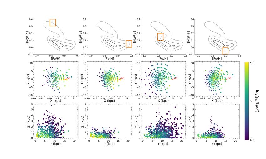
Figure 7 (Figure 8) shows the radial (vertical) density single exponential profile. The distribution seems to flatten
profile of MAPs at three different heights (radii). For visual at large vertical distance (|Z| > 2 kpc) in some MAPs (e.g.,
clarity, an arbitrary density offset is added to the data points [Fe/H]=-0.4, [Mg/Fe]=0.05), but more observations far off
denoted in orange and magenta dots. Enlarged squares rep- the disc will be needed to draw a more affirmtive conclusion.
resent the median number density as a function of radius or The vertical density distribution tend to be flatter with in-
height, and are included to highlight the shape of density creasing radius in many MAPs, which is usually referred to
profiles. as the ‘flaring’ feature in the disc (§4.3).
Surprisingly, most MAPs, including many high-α MAPs
with [Mg/Fe]> 0.2, display a non-linear shape in their radial
4.3 Radial variation of scale height
density distribution in logarithm, with a break near the solar
radius and a flatter distribution in the inner Galaxy. This Before performing a full parametric fitting to the density
non-linear profile shape seems to be present in the radial distribution ρ(R, |Z|), we first measure the scale height in a
density profile of stars with different colours in Jurić et al. series of narrow radial bins from 0 to 15 kpc (∆R = 1 kpc).
(2008), which was interpreted as a wide overdensity feature. A single exponential profile is used to fit the vertical den-
A broken radial density distribution with two exponential sity distribution up to 4 kpc in each radial bin. Figure 9
profiles was used by Bovy et al. (2016b) and Mackereth et al. shows the best-fitted scale height as a function of radius for
(2017) to fit the APOGEE data and by Yu et al. (2021) for each MAP. Most MAPs, except for those with [Mg/Fe]< 0,
LAMOST data. With the latest APOGEE observations, we exhibit a clear trend of increasing scale height (i.e. thick-
directly recover the density distribution of underlying pop- ness) with radius (i.e., flare). Surprisingly, the high-α pop-
ulations and confirm the presence of a broken radial density ulations display the steepest increase of scale height with
profile. Given the radial extent of the ‘flat’ part of the dis- radius, i.e., the strongest flaring. This is at odds with the
tributions, it seems that the broken radial profile is unlikely finding in Bovy et al. (2016b) of a constant thickness of high-
to be caused by an overdensity structure in the disc. It is α stars, but more consistent with the recent work by Yu
always possible that the profile density break near the solar et al. (2021) using LAMOST data. Yu et al. (2021) showed
radius measured here and by others is due to some observa- that both the high- and low-α MAPs flare with comparable
tional bias. However, there are also reasons that a break here strength. Another interesting finding in Yu et al. (2021) is
is physically plausible. For example, a possible origin of this that the flaring in low-α MAPs occurs mostly at R > 10 kpc.
broken radial profile is the presence of outer Lindbald Res- Such flaring pattern of low-α stars seems also present in
onance (OLR), which limits churning migration across this some low-α MAPs in Fig. 9 (e.g., MAP at [Fe/H]=-0.4 and
radius and therefore separate the disc into two parts with [Mg/Fe]=0.15).
little exchange as found in the simulation by Halle et al.
(2015). It is suggested that the current position of the OLR
of the Milky Way is slightly inside the solar radius (Dehnen 5 STRUCTURE OF MONO-ABUNDANCE
2000; Famaey et al. 2005; Minchev et al. 2007), close to the POPULATIONS
position of the break seen in the radial density profile. It is
also interesting to note that the chemical properties of the To quantitatively compare the structure between various
outer disc (R > 10 kpc) are substantially different from the MAPs, we perform a 2D parametric fitting to the intrin-
inner disc (e.g., Haywood et al. 2013; Anders et al. 2014; sic density distribution of each MAP, in radius and vertical
Nidever et al. 2014), which may also be caused by the exis- distance simultaneously.
tence of OLR (Halle et al. 2015).
It is interesting to note that in external disc galaxies
5.1 Density model
with deep imaging data, a broken radial density profile with
two distinct exponential components is frequently seen (e.g., The density model adopted from Bovy et al. (2016b) has
Pohlen et al. 2002; Pohlen & Trujillo 2006). For example, also been used to derive the structure parameters of mono-10 J. Lian et al.
Figure 7. Radial density profile of mono-abundance populations at three |Z| height bins as illustrated in the top-right legend. Small
dots indicate intrinsic density measurements at each location. Enlarged symbols show the median intrinsic density at various radial bins
with bin size of 2 kpc. To better visualize the profile at different heights, an arbitrary negative shift in y-axis is added to the two height
bins above the disc plane. The solid lines represent the best-fitted density model that will be discussed in §5.1 below.
Figure 8. Similar to Fig. 7 but showing the vertical density profile at three radial bins. An arbitrary negative shift in y-axis is added to
the two radial bins in orange and magenta.
age or mono-abundance populations in many other works length inside and outside the break radius (hR,inner and
(e.g., Mackereth et al. 2017; Yu et al. 2021). It consists of hR,outer ).
two components, which describes the density distribution in
radial and vertical direction separately. (
eR/hR,inner R 6 Rb
ρ(R, |Z|) ≡ υ(R)ζ(R, |Z|), (4) υ(R) ∝
e−R/hR,outerr R > Rb
The radial component is a broken exponential profile
with three free parameters: break radius (Rb ), and the scale The vertical component in the density model is a sin-Density distribution and structure of MAPs 11
Figure 9. Scale height of mono-abundance populations as a function of radius. Error bars indicate the uncertainties of scale height
estimated via Monte Carlo simulation. Dashed lines indicate the prediction of 2D density model (§5.1).
gle exponential profile. Based on the analysis in §4.3 and sity distribution of MAPs in both radial and vertical di-
Fig. 9, we set the scale height as a linear function of radius rection. For example, the broken radial density profile of
as following: low-α MAPs are well reproduced by the model with double
exponential components in radius. Note that individual in-
ζ(R, |Z|) ∝ e−|Z|/hZ (R) , hZ (R) = Aflare × (R − R ) + hZ,R trinsic density measurements are more frequent close to Sun
(5) because of the adopted binning in distance. The good match
The slope of this linear function (Aflare ) represents the between the model prediction and the observed median ra-
strength of flaring, and the intercept is the scale height at dial and vertical density profiles suggests that the concen-
the solar radius, which are both set to be free. The density tration of density measurements at solar vicinity does not
model is scaled to the number density at the solar radius significantly affect the result.
in the disc plane, which is the last free parameter in the
model. In this work, we adopt a solar position in the Galaxy
of R = 8.2 kpc and Z = 0.027 kpc (Bland-Hawthorn &
Gerhard 2016). There are deviations in some MAPs, which might sug-
To summarize, there are six free parameters in the den- gest interesting sub-structures that are not included in the
sity model adopted in this work: smooth density model. For instance, in many low-α MAPs,
the intrinsic number density is higher than predicted close
• ρ , intrinsic density at solar radius on the disc plane, to Galactic center (R < 4 kpc). This feature is not captured
• Rb , break radius in the radial density distribution, by the model and may be signature of the bar in the inner
• hR,inner , scale length at R 6 Rb , Galaxy.
• hR,outer , scale length at R > Rb ,
• Aflare , slope of radial variation in scale height,
• hZ,R , scale height at solar radius.
The predicted radial variation of scale height of the 2D
We fit the density model simultaneously to all the spa- density model is shown as dashed line in Fig 9. It can be
tial intrinsic density measurements in a given MAP using seen that it matches well the scale height derived from 1D
curve fit function in the optimize module of SciPy (Virta- fitting in narrow radial bins, confirming the robustness of
nen et al. 2020). the 2D density fitting approach used in this work. The in-
The solid lines in Fig. 7 and Fig. 8 show the the pre- teresting non-linear radial variation of scale height in some
dicted 1D density profile of best-fitted models, which is low-α MAPs is not reproduced by our 2D model which as-
sliced from the 2D model at the median height or radius sumes linear flaring. To reproduce this feature requires a dif-
of the density measurements from which the observed me- ferent (e.g., exponential flaring in Bovy et al. (2016b) and
dian profiles are drawn. For example, to compare with the Mackereth et al. (2017)) or a more complex (e.g., step-wise)
observed median radial density profile at |Z|12 J. Lian et al.
Table 1. Best-fitted structure parameters of individual MAPs.
[Fe/H], [Mg/Fe] ρ ,N Rb hR,outer Aflare hZ,R=R
log(Number/kpc3 ) kpc kpc - kpc
-0.4,-0.05 6.149±0.066 5.09±0.816 1.961±0.178 0.028±0.02 0.525±0.074
-0.2,-0.05 6.662±0.03 8.193±0.107 1.722±0.075 0.003±0.005 0.374±0.014
0.0,-0.05 7.049±0.025 8.366±0.074 1.075±0.035 0.008±0.003 0.328±0.009
0.2,-0.05 6.961±0.07 7.826±0.25 0.8±0.044 0.019±0.017 0.293±0.084
0.4,-0.05 6.432±0.067 6.788±1.124 1.525±0.268 0.0±0.007 0.339±0.03
-0.6,0.05 5.911±0.033 5.921±0.496 4.232±0.282 0.033±0.009 0.908±0.066
-0.4,0.05 6.631±0.089 8.85±1.532 2.42±0.498 0.041±0.007 0.485±0.019
-0.2,0.05 7.142±0.024 8.317±0.096 1.743±0.05 0.017±0.002 0.378±0.007
0.0,0.05 7.253±0.015 8.06±0.042 1.23±0.025 0.02±0.001 0.371±0.007
0.2,0.05 6.993±0.018 6.776±0.079 1.206±0.03 0.02±0.002 0.376±0.01
0.4,0.05 6.554±0.034 5.956±2.408 1.42±0.165 0.012±0.007 0.36±0.013
-0.6,0.15 5.886±0.028 0.643±2.158 4.225±0.194 0.084±0.006 0.862±0.035
-0.4,0.15 6.396±0.032 7.935±0.77 2.511±0.12 0.042±0.004 0.699±0.018
-0.2,0.15 6.477±0.025 6.737±0.231 1.601±0.05 0.036±0.004 0.647±0.019
0.0,0.15 6.464±0.023 6.041±0.208 1.52±0.063 0.034±0.003 0.573±0.018
0.2,0.15 6.297±0.031 0.559±1.054 1.943±0.09 0.033±0.004 0.463±0.02
0.4,0.15 6.131±0.084 0.131±0.458 2.534±0.303 0.024±0.006 0.405±0.051
-0.8,0.25 5.891±0.057 0.576±2.093 3.222±0.293 0.073±0.016 0.941±0.063
-0.6,0.25 6.081±0.038 4.178±1.504 2.084±0.111 0.083±0.017 0.987±0.041
-0.4,0.25 6.359±0.018 5.533±0.219 1.623±0.046 0.064±0.005 0.886±0.023
-0.2,0.25 6.441±0.021 5.276±0.473 1.549±0.056 0.04±0.005 0.665±0.017
0.0,0.25 6.059±0.041 0.694±0.219 2.216±0.134 0.039±0.006 0.575±0.037
-0.8,0.35 5.953±0.032 0.693±0.226 2.766±0.158 0.061±0.008 0.95±0.039
-0.6,0.35 6.076±0.021 1.099±0.629 1.974±0.061 0.097±0.008 1.116±0.039
-0.4,0.35 6.082±0.025 0.724±1.248 1.951±0.059 0.082±0.01 0.932±0.034
-0.2,0.35 6.15±0.053 1.015±0.886 3.134±0.328 0.031±0.007 0.579±0.032
Figure 10. Distribution of best-fitted structure parameters in number density of mono-abundance populations in [Fe/H]-[Mg/Fe]. Each
pixel indicates one mono-abundance population. Since a single exponential profile is used in the radial component of the density model
for the high- and intermediate-α mono-abundance populations, the distribution of Rb and hR,inner in the middle and right top two panels
are only populated by the low-α populations.Density distribution and structure of MAPs 13
Figure 11. Uncertainties of best-fitted structural parameters for each estimated via Monte Carlo simulation. The uncertainty of derived
intrinsic number density of the underlying population at each spatial bin is propagated from the uncertainty of the observed number
density which is assumed to be Poisson error.
5.2 Structure parameters of number density hR,inner : The slope of the radial density distribution
distribution of MAPs in the inner Galaxy is consistently flat (hR,inner
generally greater than 100), in contrast to the rapid decrease
Figure 10 and Figure 11 present the distribution of the best-
beyond the break radius. Since hR,inner presents no clear
fitted parameters in [Fe/H]-[Mg/Fe] and their stochastic un-
dependence on [Fe/H] and [Mg/Fe], this parameter is not
certainties estimated through Monte Carlo simulation. Pois-
included in Figs. 10-13.
son error is assumed for the observed number density at each
spatial bin, which is then propagated to the derived intrinsic hR,outer : The slope of the radial density distribution
density of the underlying population. Each pixel corresponds beyond the break radius presents a complicated distribution
to one MAP. The best-fitted parameters are also listed in in abundance space. Interestingly, there is a similar trend of
Table 1. flatter radial density distribution at lower [Fe/H] in both
ρ ,N : The local intrinsic number density of MAPs dis- high- and low-α MAPs. The origin of this trend is unclear,
play large variations more than an order of magnitude with but not likely driven by radial migration. For high-α popu-
uncertainties less than 0.1 dex. The most common stars in lations, they are generally old and have similar ages across
the solar vicinity tend to have solar-like abundances, while metallicities. If they have experienced radial migration, the
the least numerous stars here are in the high-α sequence, strength of migration should be similar. For low-α popula-
with a decreasing number density at lower [Fe/H]. This tions, their age does not monotonically correlate with the
selection-function corrected density distribution is qualita- their [Fe/H] (e.g., Anders et al. 2017; Feuillet et al. 2018).
tively consistent with that seen in raw APOGEE data (e.g., In fact, the most metal-rich stars are actually the oldest
Hayden et al. 2015), confirming that APOGEE data have population on average. However these metal-rich stars ex-
no significant selection bias on chemical abundances (Rojas- hibit shorter outer scale length compared to low-α MAPs
Arriagada et al. 2019). with [Fe/H]< −0.1, the opposite of what is expected if they
Rb : The break radius of the broken radial profile is have experienced more radial migration. The different outer
largest in low-α MAPs with sub-solar metallicities, smaller scale length of the radial density distribution in the high-
in the super-solar metallicity, low-α MAPs and the small- α and metal-rich, low-α populations suggest that they are
est in the high-α MAPs. Given the mean age of different not always physically associated at all radii of the Galaxy.
MAPs, this indicates an age dependence of break radius, This can be explained in disc formation models where the
with a larger break radius in younger population, and re- star formation and chemical evolution during the thick-to-
flects radial expansion of the Milky Way’s disc throughout thin disc transition is radially dependent (Chiappini 2009;
its history, also known as inside-out growth of the disc (e.g., Sharma et al. 2020, Lian et al. in prep). Note that the shorter
Frankel et al. 2019). The typical break radius of external outer scale length in metal-rich, low-α populations than the
galaxies with downbending broken profile (steeper outer re- high-α stars is not at odds with their similar radial extent
gion) is generally between 5-15 kpc (Pohlen & Trujillo 2006), as shown in Fig. 6, since the low-α populations have a larger
comparable to the break radius we find here in the Milky break radius.
Way. Aflare : This parameter characterizes the strength of14 J. Lian et al.
flaring, which is defined here to be the slope of radial vari- 6 DISCUSSION
ation in scale height. The high-α MAPs generally flare,
6.1 Comparing to previous MAP studies
with the strongest flaring at [Fe/H]= −0.6 and decreasing
strength at lower and higher [Fe/H]. This is different from In this section we discuss our best-fitted MAP structural pa-
the constant thickness of high-α populations reported in rameters in comparison with previous observational (Bovy
Bovy et al. (2016b), but broadly consistent with the results et al. 2012b, 2016b; Mackereth et al. 2017; Yu et al. 2021)
in Mackereth et al. (2017) and Yu et al. (2021) where a flar- and theoretical MAP studies (Bird et al. 2013; Stinson et al.
ing high-α disc was also found although with less strength 2013; Minchev et al. 2015). The absolute scale and global
than the low-α disc. In the low-α MAPs, the super-solar shapes of radial and vertical density distributions are in good
and solar-abundance stars present negligible flaring, while agreement with previous works using early APOGEE (Bovy
stars at lower [Fe/H] flare with moderate strength that is et al. 2016b; Mackereth et al. 2017) or LAMOST data (Yu
less than the high-α stars. et al. 2021). Many newly discovered features, such as broken
hZ,R=R : The scale height of MAPs at solar circle show radial density distribution of low-α MAPs and flaring high-
a clear trend of decreasing thickness with lower [Mg/Fe]. α MAPs, are confirmed in this work. Nevertheless, there are
Similar to the radial variation of scale height. The MAP with notable differences from earlier works in some structural pa-
[Fe/H]= −0.6 and [Mg/Fe]= 0.35 stands out with the widest rameters. One of the most striking results in this work is the
vertical density distribution and a scale height of ∼1.1 kpc, structure of high-α disc, which presents a broken radial den-
while the solar-abundance stars are the most confined to the sity distribution similar to the low-α disc and the strongest
disc plane with scale height ∼0.3 kpc. flaring among all MAPs. This new result may provide valu-
able insights into the thick disc formation of the Milky Way.
More detailed comparison on each aspect of MAPs’ struc-
ture, from the local mass density to the radial and vertical
structure, is given below.
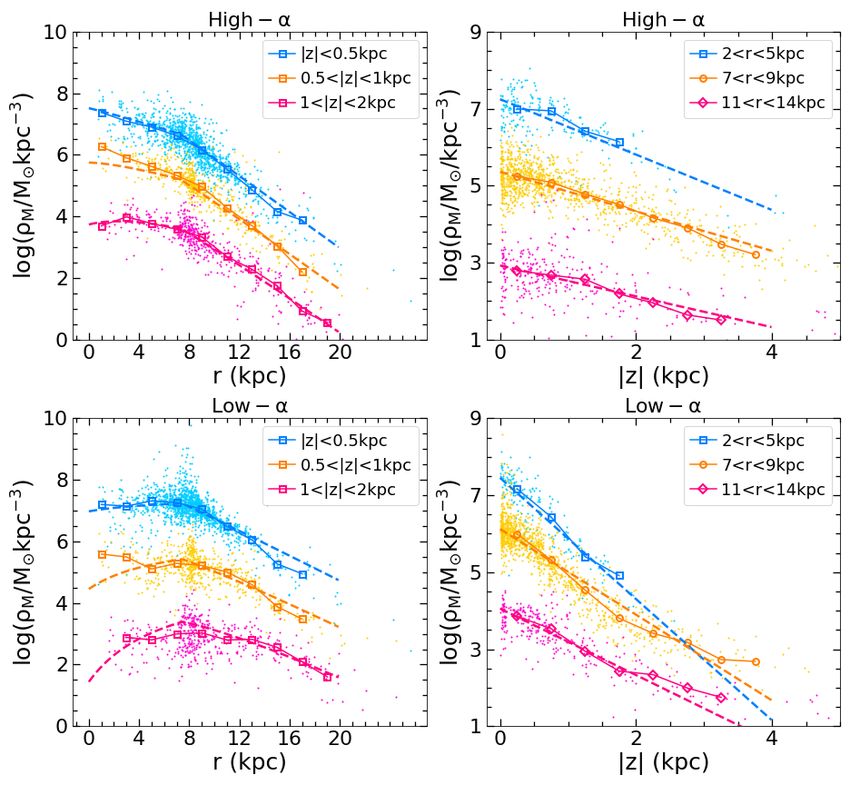
6.1.1 Local mass density
Mackereth et al. (2017) derived the local surface mass den-
5.3 Structure parameters of mass and luminosity sity near the solar circle as a function of age and [Fe/H],
density distribution and find the highest surface density in the youngest age,
In addition to the intrinsic number density that is directly solar-[Fe/H] population. This is consistent with our result
recovered from the data, it is also interesting to explore the of highest local density at solar-[Fe/H] and solar-[Mg/Fe],
spatial distribution of mass and luminosity of MAPs, which which is the MAP with the youngest average age (Fig. 1).
allows more direct comparison with the structure of Milky In the next section we will present our surface mass density
Way in the literature. Moreover, the obtained intrinsic mass measurements for integrated high- and low-α populations
and luminosity density distributions will lay the foundation and perform a more quantitative comparison with the re-
to measure mass- and light-weighted integrated stellar popu- sults in Mackereth et al. (2017) and other non-MAP works.
lation properties of our Milky Way as we do in other galaxies
and enable direct comparison between them in the future.
6.1.2 Radial structure
The conversion from number to mass and luminosity
density is conducted by sampling the PARSEC isochrones For the radial distribution of low-α MAPs, Bovy et al.
(Bressan et al. 2012), using the age distribution presented in (2016b) suggested a broken exponential profile provides a
§2.2. For SDSS and 2MASS single band luminosities, PAR- better fit to the raw density distribution of APOGEE low-
SEC isochrones only provide absolute magnitude. To nor- α stars than a single exponential. A broken profile is also
malize to the solar luminosity, we use the solar magnitude in adopted in following MAP studies in Mackereth et al. (2017)
these filters (Willmer 2018). This sampling is performed for and Yu et al. (2021). In this work, by directly recovering the
all locations where we have number density measurements. density distribution of underlying populations, we explicitly
The obtained spatial distributions of mass and luminosity show the presence of such broken radial density distribution
density have very similar shapes to those of the number of low-α stars and also find a similar broken profile in high-α
density. stars.
We fit the spatial distributions of mass and bolomet- Bovy et al. (2016b) and Mackereth et al. (2017) found
ric/SDSS+2MASS luminosity densities of each MAP with that the break radius in low-α MAPs is anti-correlated with
the same density model and strategy as the fitting in num- [Fe/H] with a range of 6−12 kpc. This is not confirmed with
ber density. Figure 12 and Figure 13 present the distribution LAMOST data in Yu et al. (2021), in which a roughly con-
of best-fitted structure parameters for the mass and bolo- stant break radius was found. These different results might
metric luminosity of all MAPS, respectively. The structure be (partially) due to the different spatial coverage of the
of MAPs in number, mass or luminosity are indistinguish- two surveys, in particular in the inner Galaxy. In this work
able. One very minor change is the slight shift of the MAP we find the break radius peaks at ∼11 kpc in the low-α
with the highest density, from the one with [Fe/H]= 0 and MAP at [Fe/H]= −0.4 and [Mg/Fe] = 0.05 and decreases
[Mg/Fe]You can also read