THE KFIOU LOSS FOR ROTATED OBJECT DETECTION
←
→
Page content transcription
If your browser does not render page correctly, please read the page content below
Preprint 2022

                                        T HE KFI O U L OSS FOR ROTATED O BJECT D ETECTION
                                         Xue Yang1 , Yue Zhou2 , Gefan Zhang1 , Jirui Yang3 , Wentao Wang1
                                         Junchi Yan1,∗, Xiaopeng Zhang4 , Qi Tian4
                                         1
                                           Department of CSE, MoE Key Lab of Artificial Intelligence, Shanghai Jiao Tong University
                                         2
                                           Department of EE, Shanghai Jiao Tong University
                                         3
                                           University of Chinese Academy of Sciences 4 Huawei Inc.
                                         {yangxue-2019-sjtu,sjtu zy}@sjtu.edu.cn

                                                                                        A BSTRACT
arXiv:2201.12558v4 [cs.CV] 6 Oct 2022

                                                     Differing from the well-developed horizontal object detection area whereby the
                                                     computing-friendly IoU based loss is readily adopted and well fits with the detec-
                                                     tion metrics. In contrast, rotation detectors often involve a more complicated loss
                                                     based on SkewIoU which is unfriendly to gradient-based training. In this paper,
                                                     we propose an effective approximate SkewIoU loss based on Gaussian modeing
                                                     and Kalman filter, which mainly consists of two items. The first term is a scale-
                                                     insensitive center point loss, which is used to quickly get the center points between
                                                     bounding boxes closer to assist the second term. In the distance-independent sec-
                                                     ond term, Kalman filter is adopted to inherently mimic the mechanism of SkewIoU
                                                     by its definition, and show its alignment with the SkewIoU loss at trend-level
                                                     within a certain distance (i.e. within 9 pixels). This is in contrast to recent Gaus-
                                                     sian modeling based rotation detectors e.g. GWD loss and KLD loss that involve
                                                     a human-specified distribution distance metric which require additional hyperpa-
                                                     rameter tuning that vary across datasets and detectors. The resulting new loss
                                                     called KFIoU loss is easier to implement and works better compared with exact
                                                     SkewIoU loss, thanks to its full differentiability and ability to handle the non-
                                                     overlapping cases. We further extend our technique to the 3-D case which also
                                                     suffers from the same issues as 2-D detection. Extensive results on various public
                                                     datasets (2-D/3-D, aerial/text/face images) with different base detectors show the
                                                     effectiveness of our approach.

                                        1       I NTRODUCTION
                                        Rotated object detection is an relatively emerg-
                                        ing but challenging area, due to the difficul-
                                        ties of locating the arbitrary-oriented objects
                                        and separating them effectively from the back-
                                        ground, such as aerial images (Yang et al.,
                                        2018a; Ding et al., 2019; Yang et al., 2018b;
                                        Yang & Yan, 2022), scene text (Jiang et al.,
                                        2017; Zhou et al., 2017; Ma et al., 2018).
                                        Though considerable progresses have been re-
                                        cently made, for practical settings, there still
                                        exist challenges for rotating objects with large
                                        aspect ratio, dense distribution.
                                        The Skew Intersection over Union (SkewIoU) Figure 1: For rotation detection (Yang et al.,
                                        score between large aspect ratio objects is sen- 2021b), there is a notable inconsistency between
                                        sitive to the deviations of the object positions. the final detection metric i.e. mAP (largely de-
                                        This causes the negative impact of the inconsis- pending on SkewIoU) and l loss.
                                                                                                                      n
                                        tency between metric (dominated by SkewIoU)
                                        and regression loss (e.g. ln -norms), which is common in horizontal detection, and is further am-
                                        plified in rotation detection. The red and orange arrows in Fig. 1 show the inconsistency between
                                            ∗
                                                Corresponding author is Junchi Yan

                                                                                              1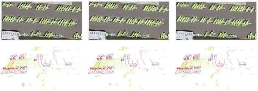
Preprint 2022

SkewIoU and Smooth L1 Loss. Specifically, when the angle deviation is fixed (red arrow), SkewIoU
will decrease sharply as the aspect ratio increases, while the Smooth L1 loss is unchanged (mainly
from the angle difference). Similarly, when SkewIoU does not change (orange arrow), Smooth L1
loss increases as the angle deviation increases. Solution for inconsistency between the metric and
regression loss has been extensively discussed in horizontal detection by using IoU loss and related
variants, such as GIoU loss (Rezatofighi et al., 2019) and DIoU loss (Zheng et al., 2020b). However,
the applications of these solutions to rotation detection are blocked because the analytical solution
of the SkewIoU calculation process is not easy to be provided due to the complexity of intersec-
tion between two rotated boxes (Zhou et al., 2019). Especially, there exist some custom operations
(intersection of two edges and sorting the vertexes etc.) whose derivative functions have not been
implemented in the existing deep learning frameworks (Abadi et al., 2016; Paszke et al., 2017).
Based on the above analysis, developing an easy-to-implement approximate SkewIoU loss is mean-
ingful and several works (Chen et al., 2020; Zheng et al., 2020a; Yang et al., 2021c;d) have been
proposed.
This paper aims to find an easy-to-implement and better-performing alternative. We design a novel
and effective alternative to SkewIoU loss based on Kalman filter, named KFIoU loss, which can be
easily implemented by the existing operations of the deep learning framework without the need for
additional acceleration (e.g. C++/CUDA). Specifically, we convert the rotated bounding box into
a Gaussian distribution, which can avoid the well-known boundary discontinuity and square-like
problems (Yang & Yan, 2020; Qian et al., 2021a; Ming et al., 2021c; Yang et al., 2021c) in rota-
tion detection. Then we use a center point loss to narrow the distance between the center of the
two Gaussian distributions, follow by calculating the overlap area under the new position through
Kalman filter. By calculating the error variance and comparing the final performance of different
methods (including L1 loss, KLD loss, GWD loss and KFIoU loss etc.), we find trend-level align-
ment with the SkewIoU loss is critical for solving the inconsistency between metric and loss, and
further improving the performance. Furthermore, compared to best-tuned Gaussian distance metric
based methods, our proposed method achieves more competitive performance without hyperparam-
eter tuning. The highlights are as follows:
1) For rotation detection, instead of exactly computing the SkewIoU loss which is tedious and un-
friendly to differentiable learning, we propose our new approximate loss – KFIoU loss. It follows
the protocol of Gaussian modeling for objects (Yang et al., 2021c;d), yet innovatively uses Kalman
filter to mimic SkewIoU’s computing mechanism within a looser distance.
2) Compared with plain SkewIoU loss, our KFIoU loss is easy-to-implement, and works better due
to fully differentiable and able to handle the non-overlapping cases. Compared to Gaussian-based
losses (GWD loss, KLD loss) that try to approximate SkewIoU loss by specifying a distance which
requiry extra hyperparameters tuning and metric selection that vary across datasets and detectors,
our mechanism level simulation to SkewIoU is more interpretable and natural, and free from hyper-
parameter tuning.
3) Compared with GWD loss and KLD loss, we show that KFIoU loss achieves the best trend-level
alignment with SkewIoU loss within a certain distance, where the trend deviation is measured by
our devised error variance. The effectiveness of such a trend-level alignment strategy is verified by
comparing KFIoU loss with ideal SkewIoU loss. On extensive benchmarks (aerial images, scene
texts, face), our approach also outperforms other best-tuned SOTA alternatives.
4) We further extend the Gaussian modeling and KFIoU loss from 2-D to 3-D rotation detection,
with notable improvement compared with baselines. To our best knowledge, this is the first 3-
D rotation detector based on Gaussian modeling which also verifies its effectiveness, which is in
contrast to (Yang et al., 2021c;d) focusing on 2-D rotation detection. The source code is available at
AlphaRotate1 and MMRotate2 .

2       R ELATED W ORK
Rotated Object Detection. Rotated object detection is an emerging direction, which attempts to
extend classical horizontal detectors (Girshick, 2015; Ren et al., 2015; Lin et al., 2017a;b) to the
    1
        https://github.com/yangxue0827/RotationDetection
    2
        https://github.com/open-mmlab/mmrotate

                                                      2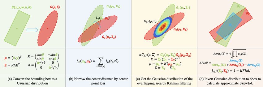
Preprint 2022

Figure 2: SkewIoU loss approximation process in two-dimensional space based on Kalman filter.
Compared with GWD loss (Yang et al., 2021c) and KLD loss (Yang et al., 2021d), our approach
follows the calculation process of SkewIoU without introducing additional hyperparameters. We
believe such a design is more mathematically rigorous and more in line with SkewIoU loss.

rotation case by adopting the rotated bounding boxes. Aerial images and scene text are popular
application scenarios of rotation detector. For aerial images, objects are often arbitrary-oriented and
dense-distributed with large aspect ratios. To this end, ICN (Azimi et al., 2018), ROI-Transformer
(Ding et al., 2019), SCRDet (Yang et al., 2019), Mask OBB (Wang et al., 2019), Gliding Vertex (Xu
et al., 2020), ReDet (Han et al., 2021b) are two-stage mainstreamed approaches whose pipeline is
inherited from Faster RCNN (Ren et al., 2015), while DRN (Pan et al., 2020), DAL (Ming et al.,
2021d), R3 Det (Yang et al., 2021b), RSDet (Qian et al., 2021a;b) and S2 A-Net (Han et al., 2021a) are
based on single-stage methods for faster detection speed. For scene text detection, RRPN (Ma et al.,
2018) employs rotated RPN to generate rotated proposals and further perform rotated bounding box
regression. TextBoxes++ (Liao et al., 2018a) adopts vertex regression on SSD (Liu et al., 2016).
RRD (Liao et al., 2018b) improves TextBoxes++ by decoupling classification and bounding box
regression on rotation-invariant and rotation sensitive features, respectively. The regression loss of
the above algorithms are rarely SkewIoU loss due to the complexity of implementing SkewIoU.
Variants of IoU-based Loss. The inconsistency between metric and regression loss is a common
issue for both horizontal detection and rotation detection. Solution for this inconsistency has been
extensively discussed in horizontal detection by using IoU related loss. For instance, Unitbox (Yu
et al., 2016) proposes an IoU loss which regresses the four bounds of a predicted box as a whole
unit. More works (Rezatofighi et al., 2019; Zheng et al., 2020b) extend the idea of Unitbox by
introducing GIoU (Rezatofighi et al., 2019) and DIoU (Zheng et al., 2020b) for bounding box re-
gression. However, their applications to rotation detection are blocked due to the hard-to-implement
of the SkewIoU. Recently, some approximate methods for SkewIoU loss have been proposed.
Box/Polygon based: SCRDet (Yang et al., 2019) propose IoU-Smooth L1, which partly circum-
vents the need for SkewIoU loss with gradient backpropagation by combining IoU and Smooth L1
loss. To tackle the uncertainty of convex caused by rotation, the work (Zheng et al., 2020a) proposes
a projection operation to estimate the intersection area for both 2-D/3-D object detection. PolarMask
(Xie et al., 2020) proposes Polar IoU loss that can largely ease the optimization and considerably im-
prove the accuracy. CFA (Guo et al., 2021) proposes convex hull based CIoU loss for optimization
of point based detectors. Pixel based: PIoU (Chen et al., 2020) calculates the SkewIoU directly by
accumulating the contribution of interior overlapping pixels. Gaussian based: GWD (Yang et al.,
2021c) and KLD (Yang et al., 2021d) simulate SkewIoU by Gaussian distance measurement.

3   BACKGROUND ON G AUSSIAN M ODELING

This section presents the preliminary according to (Yang et al., 2021c), for how to convert an
arbitrary-oriented 2-D/3-D bounding box to a Gaussian distribution G(µ, Σ).

                                   Σ =RΛR> , µ = (x, y, (z))>                                       (1)

where R represents the rotation matrix, and Λ represents the diagonal matrix of eigenvalues.

                                                  3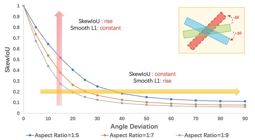
Preprint 2022
Table 1: Comparison of the properties and performance of different regression losses. Base model
is RetinaNet. BC and HP denote Boundary Continuity and Hyperparameter. † indicates that the first
term of KLD is taken as the center point loss, i.e. Lc (µ1 , µ2 , Σ1 ).
Loss Representation Implement BC Consistency HP EVar↓ DOTA-v1.0 DOTA-v1.5 DOTA-v2.0
Smooth L1 bbox easy × × X (σ) 0.073201718 64.17 56.10 43.06
plain SkewIoU bbox hard X X × - 68.27 59.01 45.87
GWD Gaussian easy X × X (τ , f ) 0.019041297 68.93 60.03 46.65
KLD Gaussian easy X X X (τ , f ) 0.007653582 71.28 62.50 47.69
KFIoU (ours) Gaussian easy X X × 0.002348353 70.64 62.71 48.04
KFIoU† (ours) Gaussian easy X X × 0.002264243 71.60 63.75 48.94
(a) Angle difference case. (b) Aspect ratio case. (c) Regardless of the case.
Figure 3: Behavior comparison of different losses in different cases. (a) depicts the relation between
angle difference and loss functions. (b) shows the changes of the five loss under different aspect
ratio condition. (c) gives scatter plot between approximate losses and SkewIoU loss, 1,000 examples
regardless of the case by randomly generating box pairs with the close centers (within 5 pixels).
For 2-D object B2d (x, y, w, h, θ),
!
w2
cos θ − sin θ 4
0
R= , Λ= h2
(2)
sin θ cos θ 0 4
and for 3-D object B3d (x, y, z, w, h, l, θ),
2
w
cos θ − sin θ 0 0 0
4 h2
R = sin θ cos θ 0 , Λ= 0 (3)
4
0
0 0 1 0 0 l2
4
and l, w, h represent the length, width, and height of the 3-D bounding box, respectively.
It is worth noting that the recent works GWD loss (Yang et al., 2021c) and KLD loss (Yang et al.,
2021d) also belong to the Gaussian modeling based. Compared with our work, their difference is
that they use the nonlinear transformation of distribution distance to approximate SkewIoU loss. In
this process, additional hyperparameters are introduced. Since Gaussian modeling has the natural
advantages of being immune to boundary discontinuity and square-like problems, in this paper, we
will take another perspective to approximate the SkewIoU loss to better train the detector without
any extra hyperparameter, which can be more in line with SkewIoU calculation. Tab. 1 shows the
comparison of properties between different losses. It should be noted that the results presented in
our experiments of GWD loss and KLD loss are obtained by best-tuned hyperparameters in DOTA,
but not optimal in others.
4 P ROPOSED M ETHOD
In this section, we present our main approach. Fig. 2 shows the approximate process of SkewIoU
loss in two-dimensional space based on Kalman filtering. Briefly, we first convert the bounding box
to a Gaussian distribution as discussed in Sec. 3, and move the center points of the two Gaussian
distributions to make them close. Then, the distribution function of the overlapping area is obtained
by Kalman filtering. Finally, the obtained distribution function is inverted into a rotated bounding
box to calculate the overlapping area and the SkewIoU and loss.
4Preprint 2022
4.1 S KEW I O U BASED ON K ALMAN F ILTERING
First of all, we can easily calculate the volume of the corresponding rotating box based on its co-
variance (VB (Σ)), when we obtain a new Gaussian distribution:
qY 1 1
VB (Σ) = 2n eig(Σ) = 2n · |Σ 2 | = 2n · |Σ| 2 (4)
where n denotes the number of dimensions.
To obtain the final SkewIoU, calculating the area of overlap is critical. For two Gaussian distribu-
tions (G1 and G2 ), we use Kalman filter3 to get the distribution function of the overlapping area:
αGkf (µ, Σ) = G1 (µ1 , Σ1 )G2 (µ2 , Σ2 ) (5)
Note here α is written by:
1 1 > −1
α = Gα (µ2 , Σ1 + Σ2 ) = p e− 2 (µ1 −µ2 ) (Σ1 +Σ2 ) (µ1 −µ2 ) (6)
det(2π(Σ1 + Σ2 ))
where µ = µ1 + K(µ2 − µ1 ), Σ = Σ1 − KΣ1 , and K is the Kalman gain, K = Σ1 (Σ1 + Σ2 )−1 .
We observe that Σ is only related to the covariance (Σ1 and Σ2 ) of the given two Gaussian dis-
tributions, which means that no matter how the two Gaussian distributions move, as long as the
covariance is fixed, the area calculated by Eq. 4 will not change (distance-independent). This is
obviously not in line with intuition: the overlapping area should be reduced when the two Gaussian
distributions are far away. The main reason is αGkf (µ, Σ) is not a standard Gaussian distribution
(probability sum is not 1), we cannot directly use Σ to calculate the area of the current overlap by
Eq. 4 without considering α. Eq. 6 shows that α is related to the distance between the center points
(µ1 − µ2 ) of the two Gaussian distributions. Based on the above findings, we can first use a center
point loss Lc to narrow the distance between the center of the two Gaussian distributions. In this
way, α can be approximated as a constant, and the introduction of the Lc also allows the entire loss
to continue to optimize the detector in non-overlapping cases. Then, calculate the overlap area under
the new position by Eq. 4. According to Fig. 2, overlap area is calculated as follow:
VB3 (Σ)
KFIoU = (7)
VB1 (Σ1 ) + VB2 (Σ2 ) − VB3 (Σ)
where B1 , B2 and B3 refer to the three different bounding boxes shown in the right part of Fig. 2.
1
In the appendix, we prove that the upper bounds of KFIoU in n-dimensional space is n . For
2 2 +1 −1
1 √ 1
2-D/3-D detection, the upper bounds are and 3 respectively when n = 2 and n = 3. We can
32−1
easily stretch the range of KFIoU to [0, 1] by linear transformation according to the upper bound,
and then compare it with IoU for consistency.
Fig. 3(a)-3(b) show the curves of five loss forms for two bounding boxes with the same center in
different cases. Note that we have expanded KFIoU by 3 times so that its value range is [0, 1] like
SkewIoU. Fig. 3(a) depicts the relation between angle difference and loss functions. Though they
all bear monotonicity, obviously the Smooth L1 loss curve is more distinctive. Fig. 3(b) shows the
changes of the five loss under different aspect ratio conditions. It can be seen that the Smooth L1
loss of the two bounding boxes are constant (mainly from the angle difference), but other losses
will change drastically as the aspect ratio varies. Regardless of the case in Fig. 3(c), KFIoU loss
can maintain the best trend-level alignment with the SkewIoU loss within 5 pixels devariation. This
conclusion still holds at 9 pixels, which is already quite a distance, especially for aerial image.
To further explore the behavior of different approximate SkewIoU losses, we design the metrics of
error mean (EMean) and error variance (EVar) as follows:
N N
1 X 1 X
EMean = (SkewIoUplain − SkewIoUapp ), EVar = (SkewIoUapp − EMean)2 (8)
N i=1 N i=1
where EVar measures the trend-level consistency between the designed loss and the SkewIoU loss.
3
We model predicted boxes, ground truth boxes, and overlapping regions into predicted values, observed
values, and uncertainties, respectively. It should be emphasized that we only borrow the technique of multiply-
ing Gaussian distributions in Kalman filter, and the rest (e.g. iterative process) is not introduced.
5Preprint 2022
Tab. 1 calculates the EVar of different losses in Fig. 3(c). In general, EVarLkf iou +Lc < EVarLkld <
EVarLgwd < EVarL1 . In our analysis, this is probably due to the fundamental inconsistency between
the distribution distance as used in GWD/KLD and the definition of similarity in SkewIoU. More-
over, for GWD such inconsistency is more pronouced, because it has no scale invariance under the
same IoU, and a case with a larger scale will get a larger loss value, it can greatly magnify its trend
inconsistency with SkewIoU loss. The results in Tab. 1 also verifies our analysis. In contrast, the
calculation process of KFIoU loss is essentially the calculation of the overlap rate, so it does not
require hyperparameters and can maintain a high trend-level consistency with SkewIoU loss.
Combined with the corresponding performance on three datasets, smaller EVars tend to have better
performance in a general level. When EVar is small enough, which implies sufficient consistency,
the performance difference of different methods (e.g. KLD loss and KFIoU loss) is close. Therefore,
we come to the conclusion that the key to maintaining the consistency between metric and regres-
sion loss lies in the trend-level consistency between approximate and exact SkewIoU loss rather
than value-level consistency. The reason why the Gaussian-based losses (e.g. KFIoU loss, KLD
loss, GWD loss) outperform the plain SkewIoU loss is due to the advanced parameter optimization
mechanism, effective measurement for non-overlapping cases, and complete derivation. However,
the introduction of hyperparameters makes KLD loss and GWD loss less stable than KFIoU loss
in terms of Evar and performance. Compared with GWD and KLD, which use the distribution dis-
tance to approximate SkewIoU, KFIoU is physically more reasonable (in line with the calculation
process of SkewIoU) and simpler, as well as empirically more effective than best-tuned GWD and
KLD. In addition, KFIoU implementation is much simpler than plain SkewIoU and can be easily
implemented by the existing operations of the deep learning framework.
4.2 T HE P ROPOSED KFI O U L OSS
We take 2-D object detection as the main example for notation brevity, though our experiments
further cover the 3-D case. We use the one-stage detector RetinaNet (Lin et al., 2017b) as the
baseline. Rotated rectangle is represented by five parameters (x, y, w, h, θ). First, we shall clarify
that the network has not changed the output of the original regression branch, that is, it is not directly
predicting the parameters of the Gaussian distribution. The whole training process of detector is
summarized as follows: i) predict offset (t∗x , t∗y , t∗w , t∗h , t∗θ ); ii) decode prediction box; iii) convert
prediction box and target ground-truth into Gaussian distribution; iv) calculate Lc and Lkf of two
Gaussian distributions. Therefore, the inference time remains unchanged. The regression equation
of (x, y, w, h) is as follows:
tx = (x − xa )/wa , ty = (y − ya )/ha , tw = log(w/wa ), th = log(h/ha )
(9)
t∗x ∗
= (x − xa )/wa , t∗y ∗
= (y − ya )/ha , t∗w ∗
= log(w /wa ), th = log(h∗ /ha )
∗
where x, y, w, h denote the box’s center coordinates, width and height, respectively. x, xa , x∗ are
for ground-truth box, anchor box, and predicted box (likewise for y, w, h).
For the regression of θ, we use two forms as the baselines:
i) Direct regression, marked as Reg. (∆θ). The model directly predicts the angle offset t∗θ :
tθ = (θ − θa ) · π/180, t∗θ = (θ∗ − θa ) · π/180 (10)
ii) Indirect regression, marked as Reg.∗ (sin θ, cos θ). The model predicts two vectors (t∗sin θ and
t∗cos θ ) to match the two targets from the ground truth (tsin θ and tcos θ ):
tsin θ = sin (θ · π/180), tcos θ = cos (θ · π/180), t∗sin θ = sin (θ∗ · π/180), t∗cos θ = cos (θ∗ · π/180)
(11)
To ensure that t∗2 ∗2
sin θ +tcos θ = 1 is satisfied, we will perform the following normalization processing:
t∗ t∗
t∗sin θ = p ∗2 sin θ ∗2 , t∗cos θ = p ∗2 cos θ ∗2 (12)
tsin θ + tcos θ tsin θ + tcos θ
The multi-task loss is:
Npos N
X λ2 X
Ltotal = λ1 Lreg (G(bn ), G(gtn )) + Lcls (pn , tn ) (13)
n=1
N n=1
6Preprint 2022
Table 2: Ablation study on various 2-D datasets with different base detectors. ‘R’, ‘F’ and ‘G’
indicate random rotation, flipping, and graying. † indicates that the first term of KLD is taken as the
center point loss, i.e. Lc (µ1 , µ2 , Σ1 ). Base detector is RetinaNet.
Dataset Data Aug. Reg. Loss Hmean/AP50 Hmean/AP60 Hmean/AP75 Hmean/AP85 Hmean/AP50:95
Smooth L1 84.28 74.74 48.42 12.56 47.76
HRSC2016 R+F+G
KFIoU 84.41 (+0.13) 82.23 (+7.49) 58.32 (+9.90) 18.34 (+5.78) 51.29 (+3.53)
Smooth L1 70.98 62.42 36.73 12.56 37.89
MSRA-TD500 R+F
KFIoU 76.30 (+5.32) 69.84 (+7.42) 47.58 (+10.85) 19.21 (+6.65) 44.96 (+7.07)
Smooth L1 69.78 64.15 36.97 8.71 37.73
ICDAR2015
KFIoU 75.90 (+6.12) 69.28 (+5.13) 40.03 (+3.06) 9.18 (+0.47) 41.17 (+3.44)
Smooth L1 95.92 87.50 55.81 12.67 52.77
FDDB
F KFIoU 97.25 (+1.33) 94.89 (+7.39) 77.38 (+21.57) 25.62 (+12.93) 63.25 (+10.48)
Smooth L1 65.00 57.84 33.68 11.39 35.16
DOTA-v1.0 KFIoU 67.68 (+2.68) 62.18 (+4.34) 37.30 (+3.62) 14.21 (+2.82) 38.51 (+3.35)
KFIoU† 68.23 (+3.23) 63.23 (+5.39) 38.34 (+4.66) 13.72 (+2.33) 38.80 (+3.64)
where N and Npos indicates the number of all anchors and that of positive anchors. bn denotes the
n-th predicted bounding box, gtn is the n-th target ground-truth. G(·) is Gaussian transfer function.
tn represents the label of the n-th object, pn is the n-th probability distribution of classes calculated
by sigmoid function. λ1 , λ2 control the trade-off and are set to {0.01, 1}. The classification loss
Lcls is set as the focal loss (Lin et al., 2017b). The regression loss is set by Lreg = Lc + Lkf , where
Lkf (Σ1 , Σ2 ) = e1−KFIoU − 1 (14)
See more ablation experiments on the functional form of Lkf (Σ1 , Σ2 ) in the Appendix. For center
point loss Lc , this paper provides two different forms:
1) The loss adopted in Faster RCNN (Lin et al., 2017a) (default): Lc (t, t∗ ) = i∈(x,y) ln (ti , t∗i ).
P
2) The first term of KLD (Yang et al., 2021d) (advanced), which has an advanced center point
optimization mechanism: Lc (µ1 , µ2 , Σ1 ) = ln (µ2 − µ1 )> Σ−1
1 (µ2 − µ1 ) + 1 .
5 E XPERIMENTS
5.1 DATASETS AND I MPLEMENTATION D ETAILS
Aerial image dataset: DOTA (Xia et al., 2018) is one of the largest datasets for oriented object
detection in aerial images with three released versions: DOTA-v1.0, DOTA-v1.5 and DOTA-v2.0.
DOTA-v1.0 contains 15 common categories, 2,806 images and 188,282 instances. DOTA-v1.5 uses
the same images as DOTA-v1.0, but extremely small instances (less than 10 pixels) are also an-
notated. Moreover, a new category, containing 402,089 instances in total is added in this version.
While DOTA-v2.0 contains 18 common categories, 11,268 images and 1,793,658 instances. We
divide the images into 600 × 600 subimages with an overlap of 150 pixels and scale it to 800 ×
800. HRSC2016 (Liu et al., 2017) contains images from two scenarios with ships on sea and close
inshore. The training, validation and test set include 436, 181 and 444 images.
Scene text dataset: ICDAR2015 (Karatzas et al., 2015) includes 1,000 training images and 500
testing images. MSRA-TD500 (Yao et al., 2012) has 300 training images and 200 testing images.
They are popular for oriented scene text detection and spotting.
Face dataset: FDDB (Jain & Learned-Miller, 2010) is a dataset designed for unconstrained face
detection, in which faces have a wide variability of face scales, poses, and appearance. This dataset
contains annotations for 5,171 faces in a set of 2,845 images. We manually use 70% as the training
set and the rest as the validation set.
We use AlphaRotate (Yang et al., 2021e) for implementation, where many advanced rotation detec-
tors are integrated. Experiments are performed on a server with GeForce RTX 3090 Ti and 24G
memory. Experiments are initialized by ResNet50 (He et al., 2016) by default unless otherwise
specified. We perform experiments on two aerial benchmarks, two scene text benchmarks and one
face benchmark to verify the generality of our techniques. Weight decay and momentum are set
0.0001 and 0.9, respectively. We employ MomentumOptimizer over 4 GPUs with a total of 4 im-
ages per mini-batch (1 image per GPU). All the used datasets are trained by 20 epochs, and learning
7Preprint 2022
Table 3: Results on KITTI val split 3D detection.
mAP Car - 3D Detection Ped. - 3D Detection Cyc. - 3D Detection
Method
Mod. Easy Mod. Hard Easy Mod. Hard Easy Mod. Hard
PointPillars 61.34 85.66 75.48 68.39 55.46 48.69 43.71 79.37 59.84 55.92
+ KFIoU 64.98 86.45 76.49 74.41 58.11 54.22 49.53 82.68 64.23 60.07
mAP Car - BEV Detection Ped. - BEV Detection Cyc. - BEV Detection
Method
Mod. Easy Mod. Hard Easy Mod. Hard Easy Mod. Hard
PointPillars 68.16 89.89 86.97 79.64 61.04 54.94 49.26 81.76 62.56 60.54
+ KFIoU 70.91 89.59 86.81 83.21 63.34 58.43 54.80 84.61 67.50 64.52
rate is reduced tenfold at 12 epochs and 16 epochs, respectively. The initial learning rate is 1e-3.
The number of image iterations per epoch for DOTA-v1.0, DOTA-v1.5, DOTA-v2.0, HRSC2016,
ICDAR2015, MSRA-TD500 and FDDB are 54k, 64k, 80k, 10k, 10k, 5k and 4k respectively, and
doubled if data augmentation (e.g. random graying and rotation) or multi-scale training are enabled.
KITTI (Geiger et al., 2012) contains 7,481 training and 7,518 testing samples for 3-D object detec-
tion. The training samples are generally divided into the train split (3,712 samples) and the val split
(3,769 samples). The evaluation is classified into Easy, Moderate or Hard according to the object
size, occlusion and truncation. All results are evaluated by the mean average precision with a rotated
IoU threshold 0.7 for cars and 0.5 for pedestrian and cyclists. To evaluate the model’s performance
on KITTI val split, we train our model on the train set and report the results on the val set.
We use PointPillar (Lang et al., 2019) implemented in MMDetection3D (Chen et al., 2019) as the
baseline, and the training schedule inherited from SECOND (Yan et al., 2018): ADAM optimizer
with a cosine-shaped cyclic learning rate scheduler that spans 160 epochs. The learning rate starts
from 1e-4 and reaches 1e-3 at the 60th epoch, and then goes down gradually to 1e-7 finally. In the
development phase, the experiments are conducted with a single model for 3-class joint detection.
5.2 A BLATION S TUDY AND F URTHER C OMPARISON
Ablation study on different center point losses. Tab. 1 compares the two different center point
losses proposed in Sec. 4.2 on three versions of DOTA datasets. Even with the most commonly
used Lc (t, t∗ ), KFIoU loss achieves competitive performance, significantly better than GWD loss
and comparable to KLD loss. For a fairer comparison, after adopting the same center point loss term
as KLD loss Lc (µ1 , µ2 , Σ1 ), the performance of KFIoU loss is further improved, which is better
than KLD loss thanks to a better center point optimization mechanism.
Ablation study on various 2-D
Table 4: Accuracy (%) comparison on DOTA. The bold
datasets with different detectors.
red and blue indicate the top two performances. Doc
Tab. 2 compares Smooth L1 loss and
and Dle denotes OpenCV Definition (θ ∈ [−90◦ , 0◦ )) and
KFIoU loss by indicators with different
Long Edge Definition (θ ∈ [−90◦ , 90◦ )) of RBox. ‘H’
IoU thresholds. For HRSC2016 con-
and ‘R’ denote the horizontal and rotating anchors, respec-
taining a large number of ships with
tively. † indicates that the first term of KLD is taken as the
large aspect ratios, KFIoU loss has a
center point loss, i.e. Lc (µ1 , µ2 , Σ1 ).
9.90% improvement over Smooth L1
on AP75 . For the scene text datasets Method Box Def. DOTA-v1.0 DOTA-v1.5 DOTA-v2.0
MSRA-TD500 and ICDAR2015, RetinaNet-H (Reg.) (2017b) Doc 65.73 58.87 44.16
RetinaNet-H (Reg.) (2017b) Dle 64.17 56.10 43.06
KFIoU achieves 7.07% and 3.44% RetinaNet-H (Reg.∗ ) (2017b) Dle 65.78 57.17 43.92
improvements on Hmean50:95 , reach- RetinaNet-R (Reg.) (2017b) Doc 67.25 56.50 42.04
PIoU (2020) Doc 65.85 57.65 45.23
ing 44.96% and 41.17% respectively. IoU-Smooth L1 (2019) Doc 66.99 59.16 46.31
Modulated Loss (2021a) Doc 66.05 57.75 45.17
The same conclusion can be reached Modulated Loss (2021a) Quad. 67.20 61.42 46.71
on FDDB and DOTA-v1.0 datasets. RIL (2021c)
CSL (2020)
Quad.
Dle
66.06
67.38
58.91
58.55
45.35
43.34
DCL (BCL) (2021a) Dle 67.39 59.38 45.46
Ablation study of KFIoU loss on 3- plain SkewIoU (2019) Doc 68.27 59.01 45.87
D detection. We generalize the KFIoU GWD (2021c) Doc 68.93 60.03 46.65
KLD (2021d) Doc 71.28 62.50 47.69
loss from 2-D to 3-D, with results in KFIoU (Ours) Doc 70.64 62.71 48.04
KFIoU† (Ours) Doc 71.60 63.75 48.94
Tab. 3. It involves 3-D detection and
BEV detection on KITTI val split, and
8Preprint 2022
Table 5: AP of different objects on DOTA-v1.0. R-101 denotes ResNet-101 (likewise for R-50, R-
152). RX-101 and H-104 denotes ResNeXt101 (Xie et al., 2017) and Hourglass-104 (Newell et al.,
2016). Red and blue: top two performances.
Method Backbone PL BD BR GTF SV LV SH TC BC ST SBF RA HA SP HC mAP50
PIoU (2020) DLA-34 80.90 69.70 24.10 60.20 38.30 64.40 64.80 90.90 77.20 70.40 46.50 37.10 57.10 61.90 64.00 60.50
O2 -DNet (2020) H-104 89.31 82.14 47.33 61.21 71.32 74.03 78.62 90.76 82.23 81.36 60.93 60.17 58.21 66.98 61.03 71.04
Single-stage
DAL (2021d) R-101 88.61 79.69 46.27 70.37 65.89 76.10 78.53 90.84 79.98 78.41 58.71 62.02 69.23 71.32 60.65 71.78
P-RSDet (2020) R-101 88.58 77.83 50.44 69.29 71.10 75.79 78.66 90.88 80.10 81.71 57.92 63.03 66.30 69.77 63.13 72.30
BBAVectors (2021) R-101 88.35 79.96 50.69 62.18 78.43 78.98 87.94 90.85 83.58 84.35 54.13 60.24 65.22 64.28 55.70 72.32
DRN (2020) H-104 89.71 82.34 47.22 64.10 76.22 74.43 85.84 90.57 86.18 84.89 57.65 61.93 69.30 69.63 58.48 73.23
DCL (2021a) R-152 89.10 84.13 50.15 73.57 71.48 58.13 78.00 90.89 86.64 86.78 67.97 67.25 65.63 74.06 67.05 74.06
GWD (2021c) R-152 86.96 83.88 54.36 77.53 74.41 68.48 80.34 86.62 83.41 85.55 73.47 67.77 72.57 75.76 73.40 76.30
KFIoU (Ours) R-152 89.46 85.72 54.94 80.37 77.16 69.23 80.90 90.79 87.79 86.13 73.32 68.11 75.23 71.61 69.49 77.35
CFC-Net (2021a) R-101 89.08 80.41 52.41 70.02 76.28 78.11 87.21 90.89 84.47 85.64 60.51 61.52 67.82 68.02 50.09 73.50
R3 Det (2021b) R-152 89.80 83.77 48.11 66.77 78.76 83.27 87.84 90.82 85.38 85.51 65.67 62.68 67.53 78.56 72.62 76.47
CFA (2021) R-152 89.08 83.20 54.37 66.87 81.23 80.96 87.17 90.21 84.32 86.09 52.34 69.94 75.52 80.76 67.96 76.67
Refine-stage
DAL (2021d) R-50 89.69 83.11 55.03 71.00 78.30 81.90 88.46 90.89 84.97 87.46 64.41 65.65 76.86 72.09 64.35 76.95
DCL (2021a) R-152 89.26 83.60 53.54 72.76 79.04 82.56 87.31 90.67 86.59 86.98 67.49 66.88 73.29 70.56 69.99 77.37
RIDet (2021c) R-50 89.31 80.77 54.07 76.38 79.81 81.99 89.13 90.72 83.58 87.22 64.42 67.56 78.08 79.17 62.07 77.62
S2 A-Net (2021a) R-50 88.89 83.60 57.74 81.95 79.94 83.19 89.11 90.78 84.87 87.81 70.30 68.25 78.30 77.01 69.58 79.42
R3 Det-GWD (2021c) R-152 89.66 84.99 59.26 82.19 78.97 84.83 87.70 90.21 86.54 86.85 73.47 67.77 76.92 79.22 74.92 80.23
R3 Det-KLD (2021d) R-152 89.92 85.13 59.19 81.33 78.82 84.38 87.50 89.80 87.33 87.00 72.57 71.35 77.12 79.34 78.68 80.63
R3 Det-KFIoU (Ours) Swin-T 89.50 84.26 59.90 81.06 81.74 85.45 88.77 90.85 87.03 87.79 70.68 74.31 78.17 81.67 72.37 80.90
R3 Det-KFIoU (Ours) R-152 88.89 85.14 60.05 81.13 81.78 85.71 88.27 90.87 87.12 87.91 69.77 73.70 79.25 81.31 74.56 81.03
ICN (2018) R-101 81.40 74.30 47.70 70.30 64.90 67.80 70.00 90.80 79.10 78.20 53.60 62.90 67.00 64.20 50.20 68.20
RoI-Trans. (2019) R-101 88.64 78.52 43.44 75.92 68.81 73.68 83.59 90.74 77.27 81.46 58.39 53.54 62.83 58.93 47.67 69.56
SCRDet (2019) R-101 89.98 80.65 52.09 68.36 68.36 60.32 72.41 90.85 87.94 86.86 65.02 66.68 66.25 68.24 65.21 72.61
Gliding Vertex (2020) R-101 89.64 85.00 52.26 77.34 73.01 73.14 86.82 90.74 79.02 86.81 59.55 70.91 72.94 70.86 57.32 75.02
Two-stage
Mask OBB (2019) RX-101 89.56 85.95 54.21 72.90 76.52 74.16 85.63 89.85 83.81 86.48 54.89 69.64 73.94 69.06 63.32 75.33
CenterMap (2020) R-101 89.83 84.41 54.60 70.25 77.66 78.32 87.19 90.66 84.89 85.27 56.46 69.23 74.13 71.56 66.06 76.03
CSL (2020) R-152 90.25 85.53 54.64 75.31 70.44 73.51 77.62 90.84 86.15 86.69 69.60 68.04 73.83 71.10 68.93 76.17
RSDet-II (2021a) R-152 89.93 84.45 53.77 74.35 71.52 78.31 78.12 91.14 87.35 86.93 65.64 65.17 75.35 79.74 63.31 76.34
SCRDet++ (2022) R-101 90.05 84.39 55.44 73.99 77.54 71.11 86.05 90.67 87.32 87.08 69.62 68.90 73.74 71.29 65.08 76.81
ReDet (2021b) ReR-50 88.81 82.48 60.83 80.82 78.34 86.06 88.31 90.87 88.77 87.03 68.65 66.90 79.26 79.71 74.67 80.10
Oriented R-CNN (2021) R-50 89.84 85.43 61.09 79.82 79.71 85.35 88.82 90.88 86.68 87.73 72.21 70.80 82.42 78.18 74.11 80.87
RoI-Trans.-KFIoU (Ours) Swin-T 89.44 84.41 62.22 82.51 80.10 86.07 88.68 90.90 87.32 88.38 72.80 71.95 78.96 74.95 75.27 80.93
significant performance improvements are also achieved. On the moderate level of 3-D detection,
KFIoU loss improves PointPillars by 3.64%. On the moderate level of BEV detection, KFIoU loss
achieves gains of 2.75%, at 70.91%.
Comparison with peer methods. Methods in Tab. 4 are based on the same baseline RetinaNet,
and initialized by ResNet50 (He et al., 2016) without using data augmentation and multi-scale train-
ing/testing. They are trained/tested under the same environment and hyperparameters. These meth-
ods are all published solutions to the boundary discontinuity in rotation detection.
First, we conduct ablation experiments on anchor form (horizontal and rotating anchors), rotated
bounding box definition form (OpenCV definition and Long Edge definition), and angle regression
form (direct regression and indirect regression) based on RetinaNet. Rotating anchors provides accu-
rate prior, which makes the model show strong performance in large aspect ratio objects (e.g. SV, LV,
SH). However, the large number of anchors makes it time-consuming. Therefore, we use horizontal
anchors by default to balance accuracy and speed. OpenCV definition (Doc ) (Yang et al., 2019) and
Long Edge definition (Dle ) (Ma et al., 2018) are two popular methods for defining bounding boxes
with different angles. Experiments show that Doc is slightly better than Dle on the three versions
of DOTA. Angle direct regression (Reg.) always suffers from the standing boundary discontinu-
ity problem as widely studied recently (Yang & Yan, 2020). In contrast, angle indirect regression
(Reg∗ .) is a simpler way to avoid above issues and brings performance boost according to Tab. 4.
PIoU calculates the SkewIoU by accumulating the contribution of interior overlapping pixels but the
effect is not significant. IoU-Smooth L1 partly circumvents the need for SkewIoU loss with gradient
backpropagation by combining IoU and Smooth L1 loss. Although IoU-Smooth L1 has achieved
an improvement of 1.26%/0.29%/2.15% on DOTA-v1.0/v1.5/v2.0, the gradient is still dominated by
Smooth L1 but still worse than plain SkewIoU loss. Modulated Loss and RIL implement ordered and
disordered quadrilateral detection respectively, and the more accurate representation makes them
both have a considerable performance improvement. In particular, Modulated Loss achieves the
third highest performance on DOTA-v1.5/v2.0. CSL and DCL convert the angle prediction from
regression to classification, cleverly eliminating the boundary discontinuity problem caused by the
angle periodicity. GWD loss, KLD loss and KFIoU loss are three different regression losses based
on Gaussian distribution. The results presented in our experiments of GWD loss and KLD loss
are obtained by best-tuned hyperparameters. In contrast, KFIoU loss is free from hyperparameter
tuning and has a more stable performance increase due to a more consistent calculation process with
SkewIoU loss as the center point gets closer.
9Preprint 2022
5.3 C OMPARISON WITH THE S TATE - OF - THE -A RT
Tab. 5 compares recent detectors on DOTA-v1.0, as categorized by single-, refine-, and two-stage
based methods. Since different methods use different image resolution, network structure, training
strategies and various tricks, we cannot make absolutely fair comparisons. In terms of overall perfor-
mance, our method has achieved the best performance so far, at around 77.35%/81.03%/80.93%.
6 C ONCLUSION
We have presented a trend-level consistent approximate to the ideal but gradient-training unfriendly
SkewIoU loss for rotation detection, and we call it KFIoU loss as the Kalman filter is adopted to
directly mimic the computing mechanism of SkewIoU loss by definition. This design differs from
the distribution distance based losses including GWD loss and KLD loss which in our analysis
have fundamental difficulty in achieving trend-level alignment with SkewIoU loss without tuning
hyperparameters. Moreover, KFIoU is easier to implement and works better than plain SkewIoU
due to the effective measurement for non-overlapping cases and complete derivation. Experimental
results on both 2D and 3D cases, on various datasets, show the effectiveness of our approach.
R EFERENCES
Martı́n Abadi, Paul Barham, Jianmin Chen, Zhifeng Chen, Andy Davis, Jeffrey Dean, Matthieu
Devin, Sanjay Ghemawat, Geoffrey Irving, Michael Isard, et al. Tensorflow: A system for large-
scale machine learning. In 12th {USENIX} symposium on operating systems design and imple-
mentation ({OSDI} 16), pp. 265–283, 2016.
Seyed Majid Azimi, Eleonora Vig, Reza Bahmanyar, Marco Körner, and Peter Reinartz. Towards
multi-class object detection in unconstrained remote sensing imagery. In Asian Conference on
Computer Vision, pp. 150–165. Springer, 2018.
Kai Chen, Jiaqi Wang, Jiangmiao Pang, Yuhang Cao, Yu Xiong, Xiaoxiao Li, Shuyang Sun, Wansen
Feng, Ziwei Liu, Jiarui Xu, Zheng Zhang, Dazhi Cheng, Chenchen Zhu, Tianheng Cheng, Qijie
Zhao, Buyu Li, Xin Lu, Rui Zhu, Yue Wu, Jifeng Dai, Jingdong Wang, Jianping Shi, Wanli
Ouyang, Chen Change Loy, and Dahua Lin. MMDetection: Open mmlab detection toolbox and
benchmark. arXiv preprint arXiv:1906.07155, 2019.
Zhiming Chen, Kean Chen, Weiyao Lin, John See, Hui Yu, Yan Ke, and Cong Yang. Piou loss:
Towards accurate oriented object detection in complex environments. In European Conference
on Computer Vision, pp. 195–211. Springer, 2020.
Jian Ding, Nan Xue, Yang Long, Gui-Song Xia, and Qikai Lu. Learning roi transformer for oriented
object detection in aerial images. In Proceedings of the IEEE Conference on Computer Vision
and Pattern Recognition, pp. 2849–2858, 2019.
Andreas Geiger, Philip Lenz, and Raquel Urtasun. Are we ready for autonomous driving? the kitti
vision benchmark suite. In Proceedings of the IEEE Conference on Computer Vision and Pattern
Recognition, pp. 3354–3361. IEEE, 2012.
Ross Girshick. Fast r-cnn. In Proceedings of the IEEE International Conference on Computer
Vision, pp. 1440–1448, 2015.
Zonghao Guo, Chang Liu, Xiaosong Zhang, Jianbin Jiao, Xiangyang Ji, and Qixiang Ye. Beyond
bounding-box: Convex-hull feature adaptation for oriented and densely packed object detection.
In Proceedings of the IEEE Conference on Computer Vision and Pattern Recognition, pp. 8792–
8801, 2021.
Jiaming Han, Jian Ding, Jie Li, and Gui-Song Xia. Align deep features for oriented object detection.
IEEE Transactions on Geoscience and Remote Sensing, 2021a.
Jiaming Han, Jian Ding, Nan Xue, and Gui-Song Xia. Redet: A rotation-equivariant detector for
aerial object detection. In Proceedings of the IEEE Conference on Computer Vision and Pattern
Recognition, pp. 2786–2795, 2021b.
10Preprint 2022
Kaiming He, Xiangyu Zhang, Shaoqing Ren, and Jian Sun. Deep residual learning for image recog-
nition. In Proceedings of the IEEE Conference on Computer Vision and Pattern Recognition, pp.
770–778, 2016.
Vidit Jain and Erik Learned-Miller. Fddb: A benchmark for face detection in unconstrained settings.
2010.
Yingying Jiang, Xiangyu Zhu, Xiaobing Wang, Shuli Yang, Wei Li, Hua Wang, Pei Fu, and Zhenbo
Luo. R2cnn: rotational region cnn for orientation robust scene text detection. arXiv preprint
arXiv:1706.09579, 2017.
Dimosthenis Karatzas, Lluis Gomez-Bigorda, Anguelos Nicolaou, Suman Ghosh, Andrew Bag-
danov, Masakazu Iwamura, Jiri Matas, Lukas Neumann, Vijay Ramaseshan Chandrasekhar, Shi-
jian Lu, et al. Icdar 2015 competition on robust reading. In 2015 13th International Conference
on Document Analysis and Recognition, pp. 1156–1160. IEEE, 2015.
Diederik P Kingma and Jimmy Ba. Adam: A method for stochastic optimization. arXiv preprint
arXiv:1412.6980, 2014.
Alex H Lang, Sourabh Vora, Holger Caesar, Lubing Zhou, Jiong Yang, and Oscar Beijbom. Pointpil-
lars: Fast encoders for object detection from point clouds. In Proceedings of the IEEE Conference
on Computer Vision and Pattern Recognition, pp. 12697–12705, 2019.
Minghui Liao, Baoguang Shi, and Xiang Bai. Textboxes++: A single-shot oriented scene text
detector. IEEE Transactions on Image Processing, 27(8):3676–3690, 2018a.
Minghui Liao, Zhen Zhu, Baoguang Shi, Gui-song Xia, and Xiang Bai. Rotation-sensitive regression
for oriented scene text detection. In Proceedings of the IEEE Conference on Computer Vision and
Pattern Recognition, pp. 5909–5918, 2018b.
Tsung-Yi Lin, Piotr Dollár, Ross Girshick, Kaiming He, Bharath Hariharan, and Serge Belongie.
Feature pyramid networks for object detection. In Proceedings of the IEEE Conference on Com-
puter Vision and Pattern Recognition, pp. 2117–2125, 2017a.
Tsung-Yi Lin, Priya Goyal, Ross Girshick, Kaiming He, and Piotr Dollár. Focal loss for dense
object detection. In Proceedings of the IEEE International Conference on Computer Vision, pp.
2980–2988, 2017b.
Wei Liu, Dragomir Anguelov, Dumitru Erhan, Christian Szegedy, Scott Reed, Cheng-Yang Fu, and
Alexander C Berg. Ssd: Single shot multibox detector. In European Conference on Computer
Vision, pp. 21–37. Springer, 2016.
Ze Liu, Yutong Lin, Yue Cao, Han Hu, Yixuan Wei, Zheng Zhang, Stephen Lin, and Baining Guo.
Swin transformer: Hierarchical vision transformer using shifted windows. In Proceedings of the
IEEE International Conference on Computer Vision, 2021.
Zikun Liu, Liu Yuan, Lubin Weng, and Yiping Yang. A high resolution optical satellite image dataset
for ship recognition and some new baselines. In Proceedings of the International Conference on
Pattern Recognition Applications and Methods, volume 2, pp. 324–331, 2017.
Ilya Loshchilov and Frank Hutter. Decoupled weight decay regularization. In International Confer-
ence on Learning Representations, 2018.
Jianqi Ma, Weiyuan Shao, Hao Ye, Li Wang, Hong Wang, Yingbin Zheng, and Xiangyang Xue.
Arbitrary-oriented scene text detection via rotation proposals. IEEE Transactions on Multimedia,
20(11):3111–3122, 2018.
Qi Ming, Lingjuan Miao, Zhiqiang Zhou, and Yunpeng Dong. Cfc-net: A critical feature cap-
turing network for arbitrary-oriented object detection in remote sensing images. arXiv preprint
arXiv:2101.06849, 2021a.
Qi Ming, Lingjuan Miao, Zhiqiang Zhou, Junjie Song, and Xue Yang. Sparse label assignment for
oriented object detection in aerial images. Remote Sensing, 13(14):2664, 2021b.
11Preprint 2022
Qi Ming, Lingjuan Miao, Zhiqiang Zhou, Xue Yang, and Yunpeng Dong. Optimization for arbitrary-
oriented object detection via representation invariance loss. IEEE Geoscience and Remote Sensing
Letters, 2021c.
Qi Ming, Zhiqiang Zhou, Lingjuan Miao, Hongwei Zhang, and Linhao Li. Dynamic anchor learn-
ing for arbitrary-oriented object detection. In Proceedings of the AAAI Conference on Artificial
Intelligence, volume 35, pp. 2355–2363, 2021d.
Alejandro Newell, Kaiyu Yang, and Jia Deng. Stacked hourglass networks for human pose estima-
tion. In European Conference on Computer Vision, pp. 483–499. Springer, 2016.
Xingjia Pan, Yuqiang Ren, Kekai Sheng, Weiming Dong, Haolei Yuan, Xiaowei Guo, Chongyang
Ma, and Changsheng Xu. Dynamic refinement network for oriented and densely packed object
detection. In Proceedings of the IEEE Conference on Computer Vision and Pattern Recognition,
pp. 11207–11216, 2020.
Adam Paszke, Sam Gross, Soumith Chintala, Gregory Chanan, Edward Yang, Zachary DeVito,
Zeming Lin, Alban Desmaison, Luca Antiga, and Adam Lerer. Automatic differentiation in
pytorch. 2017.
Wen Qian, Xue Yang, Silong Peng, Junchi Yan, and Yue Guo. Learning modulated loss for rotated
object detection. In Proceedings of the AAAI Conference on Artificial Intelligence, volume 35,
pp. 2458–2466, 2021a.
Wen Qian, Xue Yang, Silong Peng, Junchi Yan, and Xiujuan Zhang. Rsdet++: Point-based modu-
lated loss for more accurate rotated object detection. arXiv preprint arXiv:2109.11906, 2021b.
Shaoqing Ren, Kaiming He, Ross Girshick, and Jian Sun. Faster r-cnn: Towards real-time object
detection with region proposal networks. In Advances in Neural Information Processing Systems,
pp. 91–99, 2015.
Hamid Rezatofighi, Nathan Tsoi, JunYoung Gwak, Amir Sadeghian, Ian Reid, and Silvio Savarese.
Generalized intersection over union: A metric and a loss for bounding box regression. In Pro-
ceedings of the IEEE Conference on Computer Vision and Pattern Recognition, pp. 658–666,
2019.
Jinwang Wang, Jian Ding, Haowen Guo, Wensheng Cheng, Ting Pan, and Wen Yang. Mask obb:
A semantic attention-based mask oriented bounding box representation for multi-category object
detection in aerial images. Remote Sensing, 11(24):2930, 2019.
Jinwang Wang, Wen Yang, Heng-Chao Li, Haijian Zhang, and Gui-Song Xia. Learning center
probability map for detecting objects in aerial images. IEEE Transactions on Geoscience and
Remote Sensing, 59(5):4307–4323, 2020.
Haoran Wei, Yue Zhang, Zhonghan Chang, Hao Li, Hongqi Wang, and Xian Sun. Oriented objects
as pairs of middle lines. ISPRS Journal of Photogrammetry and Remote Sensing, 169:268–279,
2020.
Gui-Song Xia, Xiang Bai, Jian Ding, Zhen Zhu, Serge Belongie, Jiebo Luo, Mihai Datcu, Marcello
Pelillo, and Liangpei Zhang. Dota: A large-scale dataset for object detection in aerial images.
In Proceedings of the IEEE Conference on Computer Vision and Pattern Recognition, pp. 3974–
3983, 2018.
Enze Xie, Peize Sun, Xiaoge Song, Wenhai Wang, Xuebo Liu, Ding Liang, Chunhua Shen, and Ping
Luo. Polarmask: Single shot instance segmentation with polar representation. In Proceedings of
the IEEE conference on computer vision and pattern recognition, pp. 12193–12202, 2020.
Saining Xie, Ross Girshick, Piotr Dollár, Zhuowen Tu, and Kaiming He. Aggregated residual trans-
formations for deep neural networks. In Proceedings of the IEEE Conference on Computer Vision
and Pattern Recognition, pp. 1492–1500, 2017.
Xingxing Xie, Gong Cheng, Jiabao Wang, Xiwen Yao, and Junwei Han. Oriented r-cnn for object
detection. In Proceedings of the IEEE International Conference on Computer Vision, pp. 3520–
3529, 2021.
12Preprint 2022
Yongchao Xu, Mingtao Fu, Qimeng Wang, Yukang Wang, Kai Chen, Gui-Song Xia, and Xiang
Bai. Gliding vertex on the horizontal bounding box for multi-oriented object detection. IEEE
Transactions on Pattern Analysis and Machine Intelligence, 43(4):1452–1459, 2020.
Yan Yan, Yuxing Mao, and Bo Li. Second: Sparsely embedded convolutional detection. Sensors,
18(10):3337, 2018.
Xue Yang and Junchi Yan. Arbitrary-oriented object detection with circular smooth label. In Euro-
pean Conference on Computer Vision, pp. 677–694. Springer, 2020.
Xue Yang and Junchi Yan. On the arbitrary-oriented object detection: Classification based ap-
proaches revisited. International Journal of Computer Vision, 130(5):1340–1365, 2022.
Xue Yang, Hao Sun, Kun Fu, Jirui Yang, Xian Sun, Menglong Yan, and Zhi Guo. Automatic ship
detection in remote sensing images from google earth of complex scenes based on multiscale
rotation dense feature pyramid networks. Remote Sensing, 10(1):132, 2018a.
Xue Yang, Hao Sun, Xian Sun, Menglong Yan, Zhi Guo, and Kun Fu. Position detection and
direction prediction for arbitrary-oriented ships via multitask rotation region convolutional neural
network. IEEE Access, 6:50839–50849, 2018b.
Xue Yang, Jirui Yang, Junchi Yan, Yue Zhang, Tengfei Zhang, Zhi Guo, Xian Sun, and Kun Fu.
Scrdet: Towards more robust detection for small, cluttered and rotated objects. In Proceedings of
the IEEE International Conference on Computer Vision, pp. 8232–8241, 2019.
Xue Yang, Liping Hou, Yue Zhou, Wentao Wang, and Junchi Yan. Dense label encoding for bound-
ary discontinuity free rotation detection. In Proceedings of the IEEE Conference on Computer
Vision and Pattern Recognition, pp. 15819–15829, 2021a.
Xue Yang, Junchi Yan, Ziming Feng, and Tao He. R3det: Refined single-stage detector with feature
refinement for rotating object. In Proceedings of the AAAI Conference on Artificial Intelligence,
volume 35, pp. 3163–3171, 2021b.
Xue Yang, Junchi Yan, Qi Ming, Wentao Wang, Xiaopeng Zhang, and Qi Tian. Rethinking rotated
object detection with gaussian wasserstein distance loss. In International Conference on Machine
Learning, pp. 11830–11841. PMLR, 2021c.
Xue Yang, Xiaojiang Yang, Jirui Yang, Qi Ming, Wentao Wang, Qi Tian, and Junchi Yan. Learning
high-precision bounding box for rotated object detection via kullback-leibler divergence. Ad-
vances in Neural Information Processing Systems, 34, 2021d.
Xue Yang, Yue Zhou, and Junchi Yan. Alpharotate: A rotation detection benchmark using tensor-
flow. arXiv preprint arXiv:2111.06677, 2021e.
Xue Yang, Junchi Yan, Wenlong Liao, Xiaokang Yang, Jin Tang, and Tao He. Scrdet++: Detecting
small, cluttered and rotated objects via instance-level feature denoising and rotation loss smooth-
ing. IEEE Transactions on Pattern Analysis and Machine Intelligence, 2022.
Cong Yao, Xiang Bai, Wenyu Liu, Yi Ma, and Zhuowen Tu. Detecting texts of arbitrary orienta-
tions in natural images. In Proceedings of the IEEE Conference on Computer Vision and Pattern
Recognition, pp. 1083–1090. IEEE, 2012.
Jingru Yi, Pengxiang Wu, Bo Liu, Qiaoying Huang, Hui Qu, and Dimitris Metaxas. Oriented object
detection in aerial images with box boundary-aware vectors. In Proceedings of the IEEE Winter
Conference on Applications of Computer Vision, pp. 2150–2159, 2021.
Jiahui Yu, Yuning Jiang, Zhangyang Wang, Zhimin Cao, and Thomas Huang. Unitbox: An ad-
vanced object detection network. In Proceedings of the 24th ACM international conference on
Multimedia, pp. 516–520, 2016.
Yu Zheng, Danyang Zhang, Sinan Xie, Jiwen Lu, and Jie Zhou. Rotation-robust intersection
over union for 3d object detection. In European Conference on Computer Vision, pp. 464–480.
Springer, 2020a.
13Preprint 2022
Zhaohui Zheng, Ping Wang, Wei Liu, Jinze Li, Rongguang Ye, and Dongwei Ren. Distance-iou loss:
Faster and better learning for bounding box regression. In Proceedings of the AAAI Conference
on Artificial Intelligence, pp. 12993–13000, 2020b.
Dingfu Zhou, Jin Fang, Xibin Song, Chenye Guan, Junbo Yin, Yuchao Dai, and Ruigang Yang. Iou
loss for 2d/3d object detection. In 2019 International Conference on 3D Vision, pp. 85–94. IEEE,
2019.
Lin Zhou, Haoran Wei, Hao Li, Wenzhe Zhao, Yi Zhang, and Yue Zhang. Arbitrary-oriented object
detection in remote sensing images based on polar coordinates. IEEE Access, 8:223373–223384,
2020.
Xinyu Zhou, Cong Yao, He Wen, Yuzhi Wang, Shuchang Zhou, Weiran He, and Jiajun Liang. East:
an efficient and accurate scene text detector. In Proceedings of the IEEE Conference on Computer
Vision and Pattern Recognition, pp. 5551–5560, 2017.
Yue Zhou, Xue Yang, Gefan Zhang, Jiabao Wang, Yanyi Liu, Liping Hou, Xue Jiang, Xingzhao
Liu, Junchi Yan, Chengqi Lyu, Wenwei Zhang, and Kai Chen. Mmrotate: A rotated object de-
tection benchmark using pytorch. In Proceedings of the 30th ACM International Conference on
Multimedia, 2022.
A P ROOF OF KFI O U U PPER B OUND
For an n-dimensional Gaussian distribution, its volume is:
1 1
V = 2n · |Σ 2 | = 2n · |Σ| 2 (15)
For Σkf , we have
|Σkf | =|Σ1 − Σ1 (Σ1 + Σ2 )−1 Σ1 |
=|Σ1 (Σ1 + Σ2 )−1 Σ2 |
(16)
|Σ1 | · |Σ1 |
=
|Σ1 + Σ2 |
According to Minkowski’s inequality:
1 1 1
|Σ1 + Σ2 | n ≥ |Σ1 | n + |Σ2 | n (17)
Simultaneous mean inequalities:
1 1 1 1 1
|Σ1 + Σ2 | n ≥ |Σ1 | n | + |Σ2 | n ≥ 2 · |Σ1 | 2n · |Σ2 | 2n (18)
Thus: 1 1
|Σ1 | 2n · |Σ2 | 2n 1
1 ≤
|Σ1 + Σ2 | n 2
1 1
(19)
|Σ1 | 2 · |Σ2 | 2 1
≤ n
|Σ1 + Σ2 | 2
and 1 1
|Σ1 | · |Σ1 | |Σ1 | 2 · |Σ2 | 2
|Σkf | = ≤
|Σ1 + Σ2 | 2n
1 1
(20)
|Σ1 | 4 · |Σ2 | 4
1
|Σkf | ≤ 2
n
22
Combine the mean inequalities again:
1 1 1 1
1 |Σ1 | 4 · |Σ2 | 4 |Σ1 | 2 + |Σ2 | 2 (21)
|Σkf | 2 ≤ n ≤ n
2 2 2 2 +1
According to Eq. 15, we have
V1 + V2
Vkf ≤ n (22)
2 2 +1
Therefore, the upper bound of KFIoU is
Vkf 1
KFIoU = ≤ n +1 (23)
V1 + V2 − Vkf 22 − 1
When n = 2 and n = 3, the upper bounds are 31 and √32−1
1
respectively.
14Preprint 2022
Table 6: Ablation study of different KFIoU loss forms with different detectors on DOTA-v1.0.
Method Smooth L1 − ln(KFIoU + ) 1 − KFIoU e1−KFIoU − 1 e1−3KFIoU − 1 − ln(3KFIoU + )
RetinaNet 65.73 69.80 (+4.07) 70.19 (+4.46) 70.64 (+4.91) 69.64 (+3.91) –
R3 Det 70.66 72.28 (+1.62) 71.09 (+0.43) 71.58 (+0.92) – 71.77 (+1.11)
Table 7: Ablation study of training strategies and tricks. Rotate and MS indicate rotation augmenta-
tion and multi-scale training and testing.
Method KFIoU Backbone Sched. MS Rotate PL BD BR GTF SV LV SH TC BC ST SBF RA HA SP HC mAP50
R-50 12e 87.76 72.61 43.86 66.61 69.70 56.61 74.15 90.86 75.27 79.09 47.81 64.60 58.93 63.37 26.58 65.19
RetinaNet
X R-50 12e 88.90 80.68 47.12 70.40 72.20 62.49 74.84 90.91 79.63 79.73 58.54 66.40 63.67 67.13 45.33 69.86
R-50 12e 89.18 79.35 49.11 72.97 79.08 78.03 86.67 90.91 85.90 85.04 64.06 65.64 66.71 67.60 48.08 73.89
S2 A-Net
X R-50 12e 89.24 83.46 51.44 70.88 78.70 76.31 86.90 90.90 82.22 84.81 61.67 66.93 65.62 67.99 57.05 74.27
R-50 12e 89.02 81.71 53.84 71.65 79.00 77.76 87.85 90.90 87.04 85.70 61.73 64.55 75.06 71.71 62.38 75.99
X R-50 12e 89.08 82.62 53.90 71.78 78.73 77.91 87.97 90.90 86.68 85.37 63.17 67.65 74.30 71.19 61.35 76.17
Swin-T 12e 88.96 82.81 53.34 76.55 78.66 83.54 88.00 90.90 86.95 86.47 41.94 64.17 76.29 72.87 63.95 77.18
RoI Trans.
X Swin-T 12e 88.9 83.77 53.98 77.63 78.83 84.22 88.15 90.91 87.21 86.14 67.79 65.73 75.80 73.68 63.30 77.74
X R-50 24e X X 89.12 84.54 60.73 78.86 79.65 85.79 88.45 90.90 87.03 88.28 69.15 70.28 78.88 81.54 70.05 80.22
X Swin-T 12e X X 89.44 84.41 62.22 82.51 80.10 86.07 88.68 90.90 87.32 88.38 72.80 71.95 78.96 74.95 75.27 80.93
R-50 12e 89.02 74.52 47.93 69.64 77.02 74.07 82.56 90.90 79.39 83.67 59.02 62.51 63.56 65.06 37.22 70.41
X R-50 12e 89.06 73.89 49.82 68.39 78.13 75.35 86.65 90.89 82.57 83.84 59.63 62.03 66.16 66.22 47.98 72.04
X R-50 12e X 89.06 82.49 55.91 81.04 80.14 83.24 88.56 90.90 84.61 86.83 66.25 71.50 75.60 77.64 63.66 78.50
X Swin-T 12e X 89.41 83.66 56.92 79.76 80.45 84.34 88.71 90.91 85.69 87.64 67.69 72.88 76.34 73.63 72.21 79.35
R3 Det
X R-50 12e X X 89.33 84.19 58.78 81.30 80.48 84.49 88.85 90.84 85.56 87.57 69.14 70.79 77.33 80.82 66.51 79.73
X R-101 12e X X 89.28 83.32 59.40 80.29 80.43 84.70 88.85 90.87 84.51 87.95 71.86 71.60 78.31 79.42 66.60 79.83
X Swin-T 12e X X 89.24 83.75 59.77 79.40 80.95 84.61 88.84 90.84 86.86 87.93 71.71 71.17 76.79 77.42 71.59 80.06
X Swin-T 24e X X 89.50 84.26 59.90 81.06 81.74 85.45 88.77 90.85 87.03 87.79 70.68 74.31 78.17 81.67 72.37 80.90
B S UPPLEMENTARY E XPERIMENT
Ablation study of three forms of KFIoU loss on two detectors. We use two different detectors and
three different KFIoU based loss functions to verify its effectiveness, as shown in Tab. 6. RetinaNet-
based detector will have a large number of low-SkewIoU prediction bounding box in the early stage
of training, and will produce very large loss after the log function, which weakens the improvement
of the model. Compared with the linear function, the derivative of the exp-based function will pay
more attention to the training of difficult samples, so it has a higher performance, at 70.64%. In
contrast, R3 Det-based detector can generate high-quality prediction box at the beginning of training
by adding refinement stages, so it will not suffer the same troubles as RetinaNet. Due to the same
mechanism of focusing on difficult samples, log and exp-based functions are both better than linear
functions, and the best performance is achieved on the log-based function, about 72.28%. We also
expand KFIoU by 3 times to make its range truly consistent with the IoU loss, at [0, 1]. However, this
consistency do not bring any additional gains, so the following experiments are all use the KFIoU
before non-expansion.
Ablation study of training strategies and tricks. We reimplement KFIoU based on the more
powerful benchmark, MMRotate (Zhou et al., 2022). We use a single GeForce RTX 3090 Ti with
a total batch size of 2 for training. For ResNet (He et al., 2016), SGD optimizer is adopted with an
initial learning rate of 0.0025. The momentum and weight decay are 0.9 and 0.0001, respectively.
For Swin Transformer (Liu et al., 2021), AdamW (Kingma & Ba, 2014; Loshchilov & Hutter, 2018)
optimizer is adopted with an initial learning rate of 0.0001. The weight decay is 0.05. In addition,
we adopt learning rate warmup for 500 iterations, and the learning rate is divided by 10 at each
decay step. Tab. 7 performs ablation experiments on four detectors: RetinaNet (Lin et al., 2017b),
S2 A-Net (Han et al., 2021a), R3 Det (Yang et al., 2021b), and RoI Transformer (Ding et al., 2019).
The experimental results prove that KFIoU can stably enhance the performance of the detector. In
order to further improve the performance of the model on DOTA, we verified many commonly used
training strategies and tricks, including backbone, training schedule, data augmentation and multi-
scale training and testing, as shown in Tab. 7.
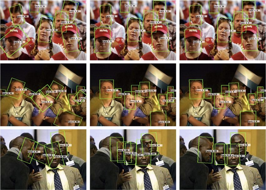
C V ISUALIZATION
Fig. 4 ad Fig. 5 show the visual comparison of three different loss functions on the different kinds
of datasets. Compared with Smooth L1 Loss, KFIoU loss is significantly better.
15You can also read