TAMP-S2GCNETS: COUPLING TIME-AWARE MUL-TIPERSISTENCE KNOWLEDGE REPRESENTATION WITH SPATIO-SUPRA GRAPH CONVOLUTIONAL NETWORKS FOR TIME-SERIES ...
←
→
Page content transcription
If your browser does not render page correctly, please read the page content below
Under review as a conference paper at ICLR 2022

TAMP-S2GCN ETS : C OUPLING T IME -AWARE M UL -
TIPERSISTENCE K NOWLEDGE R EPRESENTATION WITH
S PATIO -S UPRA G RAPH C ONVOLUTIONAL N ETWORKS
FOR T IME -S ERIES F ORECASTING

 Anonymous authors
 Paper under double-blind review

                                             A BSTRACT

         Graph Neural Networks (GNNs) are proven to be a powerful machinery for learn-
         ing complex dependencies in multivariate spatio-temporal processes. However,
         most existing GNNs have inherently static architectures, and as a result, do not ex-
         plicitly account for time dependencies of the encoded knowledge and are limited
         in their ability to simultaneously infer latent time-conditioned relations among en-
         tities. We postulate that such hidden time-conditioned properties may be captured
         by the tools of multipersistence, i.e, a emerging machinery in topological data
         analysis which allows us to quantify dynamics of the data shape along multiple
         geometric dimensions. We make the first step toward integrating the two rising
         research directions, that is, time-aware deep learning and multipersistence, and
         propose a new model, Time-Aware Multipersistence Spatio-Supra Graph Convo-
         lutional Network (TAMP-S2GCNets). We summarize inherent time-conditioned
         topological properties of the data as time-aware multipersistence Euler-Poincaré
         surface and prove its stability. We then construct a supragraph convolution mod-
         ule which simultaneously accounts for the extracted intra- and inter-dependencies
         in the data. Our extensive experiments on highway traffic flow, Ethereum token
         prices, and COVID-19 hospitalizations demonstrate that TAMP-S2GCNets out-
         performs the state-of-the-art tools in multivariate time series forecasting tasks.

1   I NTRODUCTION

Multivariate time series forecasting plays an integral role in virtually every aspect of societal func-
tioning, from biosurveillance to financial analytics to intelligent transportation solutions. In the last
few years, Graph Convolutional Networks (GCNs) have emerged as a powerful alternative to more
conventional time series predictive models. Despite their proven success, GCNs tend to be limited
in their ability to simultaneously infer latent temporal relations among entities (such as correlations
both within a time series and in-between time series or the joint spatio-temporal dependencies).
More generally, most existing GCNs architectures are inherently static and as such, do not explic-
itly account for time-conditioned properties of the encoded knowledge about the complex dynamic
phenomena.
At the same time, recent studies on integrating shape properties of the complex data into deep learn-
ing (DL) models indicate that topological representations, obtained using the tools of single param-
eter persistence, can bring an invaluable insight into the system organization and enhance the result-
ing graph learning mechanisms (Hofer et al., 2019; Carrière et al., 2020; Carlsson & Gabrielsson,
2020; Horn et al., 2021). (By shape here we broadly understand data properties which are invariant
under continuous deformations, e.g., stretching, bending, and twisting). However, in many appli-
cations, particularly, involving spatio-temporal processes, the data exhibit richer structures which
cannot be well encoded with a single parameter persistence. We postulate that many critical hid-
den time-conditioned interrelations which are inaccessible with other methods can be captured by
the emerging machinery of multipersistence. Multipersistence, or multiparameter persistence (MP)
generalizes the notion of single parameter persistence to a case when dynamics of the inherent data
shape is discerned along multiple geometric dimensions (Carlsson & Zomorodian, 2009). Despite

                                                   1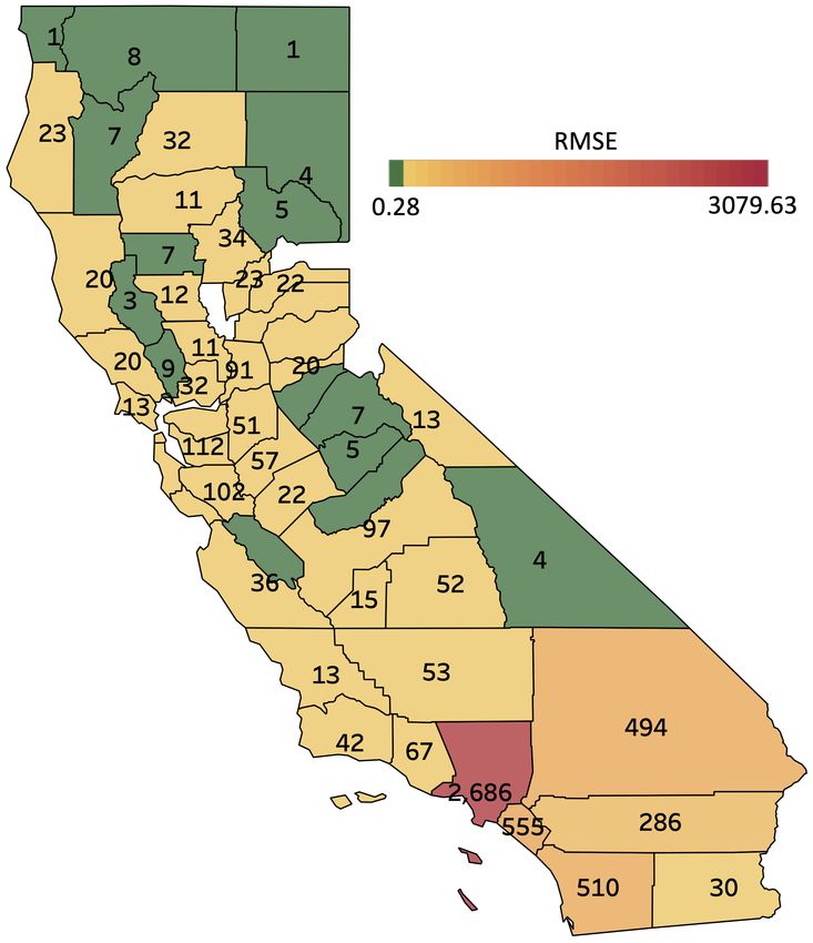
Under review as a conference paper at ICLR 2022

its premise, applications of MP in any discipline remain nascent at best (Riess & Hansen, 2020;
Kerber, 2020).
We make the first step on a path of bridging the two emerging directions, namely, time-aware DL
with time-conditioned MP representations of complex dynamic phenomena. By time-conditioned
MP representations, we mean the most salient topological properties of the data that manifest them-
selves over time. To summarize such time-conditioned topological properties, we first introduce a
dynamic Euler-Poincaré surface as a new MP summary. We then propose a directed multilayer supra
graph abstraction to represent a sequence of time-varying objects and develop a supragraph convolu-
tion module which allows us to simultaneously learn co-evolving intra- and inter-dependencies (i.e.,
spatial and temporal correlations) in the complex high-dimensional data.
The key novelty of this paper are summarized as follows:

• This is the first work to bridge the concepts of MP with the time-aware learning paradigm. Appli-
  cations of MP in any field of study are currently nascent.
• We introduce a new time-aware multipersistence invariant, a dynamic Euler-Poincaré surface. We
  prove its stability and show its substantial computational gains and high utility for encoding the
  time-conditioned knowledge.
• We propose a mathematical abstraction of directed multilayer supra graph for time-conditioned
  knowledge representation and construct a new Time-Aware Multipersistence Spatio-Supra Graph
  Convolutional Network (TAMP-S2GCNets) which simultaneously learns latent temporal inter-
  and intra-relations among entities in the complex high-dimensional data.
• We perform expansive forecasting experiments, in application to highway traffic flow, Ethereum
  token prices, and COVID-19 hospitalizations. Our findings demonstrate superior predictive per-
  formance, versatility and computational efficiency of TAMP-S2GCNets, compared to the state-
  of-the-art methods in multivariate time series forecasting.

2   R ELATED W ORKS

Multipersistence Despite that MP demonstrates very promising results in terms of improving ac-
curacy, tractability and robustness, applications of MP in ML are virtually non-existent (Wright &
Zheng, 2020; Riess & Hansen, 2020; Kerber, 2020). Some notable efforts in the direction to develop
MP summaries which are suitable for integration with ML models include Multiparameter Persis-
tence Kernel of Corbet et al. (2019), Multiparameter Persistence Landscapes (MP-L) of Vipond
(2020), and Multiparameter Persistence Images (MP-I) of Carrière & Blumberg (2020) which are
based on the concept of slicing, that is, restricting the MP module to an affine line (or single parame-
ter persistence) (Cerri et al., 2013; Landi, 2014). Such slicing methods enjoy a number of important
stability guarantees but tend to be computationally expensive even in static scenarios, which makes
them infeasible for time series forecasting tasks. In turn, the most recent results of Beltramo et al.
(2021) (i.e., Euler Characteristic Surfaces) and Coskunuzer et al. (2021) (i.e., Multiparameter Persis-
tence Grids) introduce pointwise MP representations, in application to static point clouds and graphs.
Such pointwise representations are weaker invariants but are substantially more computationally ef-
ficient. Integration of pointwise representation with ML models has not been yet investigated. Here
we propose the first time-aware pointwise MP representation, a dynamic Euler-Poincaré surface,
derive its theoretical properties and integrate it with GCN in time series forecasting tasks.
Spatial-Temporal Graph Models and Forecasting Recent studies (Li et al., 2018; Yu et al., 2018;
Yao et al., 2018) introduce graph convolution methods into spatio-temporal networks for multivari-
ate time series forecasting which, as a result, allows for better modeling of dependencies among
entities (Wu et al., 2019; Bai et al., 2020; Cao et al., 2020) and handling data heterogeneity. Despite
the GCN successes, designs of the existing spatial-temporal GCNs largely rely on the pre-defined
graph structures. As such, GCNs are restricted in their ability to explicitly integrate time dimen-
sion into the knowledge representation and learning mechanisms, thereby, limiting model adaptivity
to the dynamic environments and requiring more frequent retraining. Most recently, Chen et al.
(2021) propose a time-aware GCN, Z-GCNETs, for time series forecasting which integrates zigzag
persistence images based on a single filtration, as the primary time-conditioned topological repre-
sentation. In general, the zigzag concept can be combined with MP, but it requires more fundamental
advances in the theory of algebraic topology. As such, our time-aware MP learning approach may

                                                   2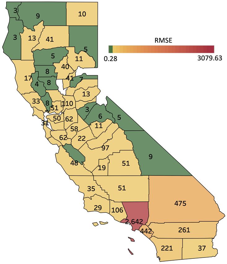
Under review as a conference paper at ICLR 2022

be viewed as complementary to zigzag persistence, while considering time-changing connections of
graph structures in dynamic networks.

3    T IME -AWARE M ULTIPERSISTENCE E ULER C HARACTERISTIC S URFACES
Spatio-Temporal Graph Construction We define a spatial network at time step t as Gt =
(Vt , Et , At , Xt ), where Vt is a set of nodes and Et is a set of edges. We let |Vt | = N and |Et | = Mt .
The adjacency matrix At ∈ RN ×N , and Xt = {xt,1 , xt,2 , . . . , xt,N }> ∈ RN ×FN is the node
feature matrix with feature dimension FN . To construct the spatial network Gt , we can build the
adjacency matrix At based on (i) the prior knowledge of graph structure: first-order neighbours, i.e.,
At,uv = 1 if the node u and node v have a connection in the dynamic graph at the time step t; and
(ii) the Radial Basis Function (RBF): degrees of similarity between instances (i.e., nodes) in Xt ,
i.e., At,uv = 1exp (−||xt,u −xt,v ||2 /γ)≤ , where γ denotes the length scale parameter and  denotes the
threshold parameter filters noisy edges. Let T be the total number of time steps. Given a sequence of
observations on a multivariate variable, X = {X1 , X2 , . . . , XT } ∈ RN ×FN ×T with T timestamps
and FN node attributes, we construct spatio-temporal networks G = {G1 , G2 , . . . , GT } via either
prior knowledge of network structure or applying RBF to the node feature matrix.
Single Parameter Persistence Persistent homology (PH) based on one parameter discerns shape
of the complex data along a single geometric dimension. The goal is to select some suitable pa-
rameter of interest and then to study a graph Gt not as a single object, but as a sequence of nested
subgraphs, or a graph filtration Gt1 ⊆ Gt2 . . . ⊆ Gtm = Gt , induced by this evolving scale pa-
rameter. Armed with such filtration, we can then assess which structural patterns (e.g., loops and
cavities) appear/disappear and record their lifespans. To make the counting process more efficient
and systematic, we build a simplicial complex Cit from each subgraph Gti , resulting in a filtration
C1t ⊆ C2t . . . ⊆ Cm t (e.g., clique complexes). For example, to construct such filtration, a common
method is to consider a filtering function f : Vt 7→ R and the corresponding increasing set of thresh-
olds {αi }m               i
           1 such that Ct = {∆ ∈ Ct : maxv∈∆ f (v) ≤ αi }. The resulting construction is called a
sublevel set filtration of f , and f can be selected, for instance, as degree, centrality, or eccentricity
function (Hofer et al., 2020; Cai & Wang, 2020). Similarly, f can be defined on the set of edges Et .
More details on a single filtration PH can be found in Appendix B.
Time-Aware Multiparameter Persistence (TAMP) Data in many applications, particularly, in-
volving spatio-temporal modeling, might be naturally indexed by multiple parameters, e.g., real
time traffic flow and optimal route in urban transportation analytics. Alternatively, the primary fo-
cus might be on discerning shape properties of the complex data along multiple dimensions. For
instance, to better predict cryptocurrency prices and manage cryptomarket investment performance,
we may need to evaluate structural patterns in cryptoasset dynamics not along one dimension but
simultaneously along the volume of transactions and transaction graph betweenness, as a measure
of joint perception of the cryptomarket volatility among the key investors. Such multidimensional
analysis of topological and geometric properties can be addressed using generalization of PH based
on a single filtration to a multifiltration case. That is, the MP idea is to simultaneously assess shape
characteristics of Gt based on a multivariate filtering function F : Vt 7→ Rd . As a result, e.g.,
for d = 2 and a set of nondecreasing thresholds {αi }m                       n
                                                               1 and {βj }1 , instead of a single filtration
                                                           αi ,βj
of complexes, we get a bifiltration of complexes {Ct              | 1 ≤ i ≤ m, 1 ≤ j ≤ n} such that if
                    αi ,βk      αi ,βl                                         α ,β
βk < βl , then Ct          ,→ Ct       and if αi < αj , then Cα    t
                                                                     i ,βk
                                                                           ,→ Ct j k . Finally, this bifiltra-
tion induces a bigraded MP module {Hk (Ctαi ,βk )}, where Hk is the k th homology group. Inspired
by Beltramo et al. (2021); Coskunuzer et al. (2021), we propose a new time-aware MP summary,
namely, a Dynamic Euler-Poincaré Surface.
Definition 3.1 (Dynamic Euler-Poincaré Surface). Let {Gt }Tt=1 be a series of time-varying graphs.
Let F = (f, g) be a multivariate filtering function F : Vt 7→ R2 with thresholds I = {(αi , βj ) |
                                       α ,β                                                          α ,β
1 ≤ i ≤ m, 1 ≤ j ≤ n}. Let Ct i j be the clique complex of the induced subgraph Gt i j =
F −1 ((−∞, αi ] × (−∞, βj ]), t = 1, 2, . . . , T and χ be the Euler–Poincaré characteristic. Then, a
                                                                                    α ,β
sequence of time-evolving m × n-matrices {Et }Tt=1 such that Etij = χ(Ct i j ) for 1 ≤ i ≤ m,
1 ≤ j ≤ n is called Dynamic Euler-Poincaré Surface (DEPS). (Figure 2 in Appendix C shows a toy
example how DEPS is computed.)
Theoretical Guarantees of DEPS Consider two graphs G + and G − , where time index t is sup-
pressed for brevity. Let F : V ± 7→ R2 be a multivariate filtering function with thresholds

                                                      3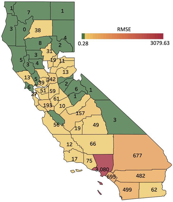
Under review as a conference paper at ICLR 2022
I = {(αi , βj ) | 1 ≤ i ≤ m, 1 ≤ j ≤ n}. Let C± be the clique complexes of G ± , and let
b ± = {C+ } be the bifiltration induced by (C± , F, I) as before. Let E± be the corresponding
C ij Pm Pn −
Euler-Poincaré Surfaces (i.e., m × n matrices). Then, set kE+ − E− k1,1 = i=1 j=1 |E+ij − Eij |
as the distance between E+ and E− , where k · k1,1 is the vectorized L1 matrix norm.
We now introduce an L1 -based MP metric instead of using L∞ -based metrics like, e.g., matching or
interleaving, due to the nature of our summaries E± (see Remark C.1 in Appendix C). Let Dkf (C± )
and Dkg (C± ) be the k th single parameter persistence diagrams (PDs) of C± for filtrations induced
by functions f, g : V ± 7→ R, respectively (see Appendix B). Let C± ±
i∗ and C∗j be clique complexes
± ±
corresponding to Gi∗ = f −1 ((−∞, αi ]) and G∗j = g −1 ((−∞, βj ]). Define the ith column dis-
g g −
tance for the k PDs as Di∗ (C , C ) = W1 (Dk (C+
th k b+ b−
i∗ ), Dk (Ci∗ )), where W1 is the Wasserstein-1
distance. Similarly, the j th row distance for k th PDs is Dk∗j (C b − ) = W1 (Df (C+ ), Df (C− )).
b +, C
k ∗j k ∗j
b ± is
Definition 3.2 (Weak L1 -metric for Multipersistence). The weak L1 -metric between C
D(C b − ) = max Dc (C
b +, C b − ), Dr (C
b +, C b −) ,
b +, C
b − ) = PM Pm Dk (C
b +, C
s.t. Dc (C b − ) and Dr (C
b +, C b − ) = PM Pn Dk (C
b +, C b − ).
b +, C
k=0 i=1 i∗ k=0 j=1 ∗j
Now, we can state our stability result for Euler-Poincaré Surfaces.
Theorem 3.1. Let G ± , F, C
b ± , E± be as defined above. Then, the Euler-Poincaré Surfaces are stable
with respect to the weak L1 -metric, i.e., kE+ − E− k1,1 ≤ C · D(C b − ) for some C > 0.
b +, C
The proof of the theorem is given in Appendix C. This stability result implies that the distances
between multiparameter PDs control the distance between the resulting Euler-Poincaré Surfaces.
By combining with the stability result for PDs (Cohen-Steiner et al., 2007), one can conclude that
the small changes in the MP filtering function F : Vt 7→ Rd or the small changes in the input data
can result only in a small change in DEPS surfaces. For further discussion on implications of the
stability result, please refer to Remark C.2.
4 T IME -AWARE M ULTIPERSISTENCE S PATIO -S UPRA G RAPH
C ONVOLUTIONAL N ETWORKS
Given T historical observations X T = {Xt−T , Xt−T +1 , . . . , Xt−1 }, the multivariate forecast-
ing model F(·) is learned to predict future observations in the next H + 1 time steps, i.e.,
{Xt , Xt+1 , . . . , Xt+H } = F(Xt−T , Xt−T +1 , . . . , Xt−1 ).
Graph Learning Architecture The graph representation learning of our MPS2GCNets is build
upon GCN. To learn node representation from graph topology and node features, the input of GCN-
based approaches contains the adjacency matrix At of the original input graph Gt and the node
feature matrix Xt . However, the prior knowledge of graph structure (1) might restrict the modeling
capacity (i.e., graph edges cannot encode the complex relationships between nodes) and (2) leads to
the neglect of neighboring information with high diversity. To avoid these limitations, inspired by
the adaptive dependency matrix (Wu et al., 2019; Chen et al., 2021), we learn the normalized self-
adaptive adjacency matrix S = {suv }N ×N with the pre-defined “cost” staying in the same node
based on the learnable node embedding Eφ = (e1,φ , e2,φ , . . . , eN,φ )> ∈ RN ×dc as
exp(ReLU(eu,φ e>
v,φ ))
P
exp(ReLU(e > , u 6= v,
u,φ ev,φ ))+exp (duu )
suv = v∈V\{u}
d
P uu
>
exp(ReLU(eu,φ ev,φ ))+exp (duu )
, u = v.
v∈V\{u}
Here hyperparameter duu is the “cost” of staying in the samePnode u and ReLU(·) = max(0, ·)
is an activation function, which guarantees suv ≥ 0. Since v suv = 1 and suv ≥ 0, we can
use S as the normalized Laplacian. Towards more effective and robust learning of both spatial and
spectral characteristics, we represent the graph diffusion as a matrix power series. That is, let S̃
be an N × N × K Laplacian tensor containing the power series {I, S, . . . , S K−1 } of S, where
I ∈ RN ×N is the identity matrix and K ≥ 2.
4Under review as a conference paper at ICLR 2022
Spatio-Temporal Feature Transformation Note that spatial and temporal domains contain inter-
dependent but highly heterogeneous types of information. Inspired by statistical factor analysis, we
facilitate signal extraction from these disparate informational sources, by mapping the original input
feature space into the high-level latent feature space, which can be written as follows
(`+1) (`)
Hi,F T = (X T Eφ ΘF T )> U , (1)
(`) dc ×P ×QFT T
where ΘF T ∈R and U ∈ R represent the learnable parameters.
4.1 S UPRAGRAPH C ONVOLUTIONAL M ODULE IN M ULTILAYER S UPRA G RAPH
We propose a novel supragraph convolutional module to simultaneously capture spatio-temporal
dependencies in dynamic networks. Our key approach is (i) to represent a sequence of time-varying
graphs recorded over a sliding time window, as a multilayer supra graph, instead of treating each
graph snapshot individually, and (ii) to learn the resulting multilayer supra graph with the random
walk exploration which allows us to encode the key details of the time-conditioned relationships
among nodes and to boost graph convolutions over multiple edge sets.
Sliding Window Historical Data as Multilayer Supra Graph Network To increase expres-
sive capability of spatio-temporal representation learning, we propose a novel directed mul-
tilayer supra graph. Particularly, we treat each graph within a sliding window G T =
{Gt−T , Gt−T +1 , . . . , Gt−1 } ∈ RN ×N ×T as a layer within a directed T -layered network. (Here
N is the number of nodes in each graph.) Since information in real world spatio-temporal pro-
cesses can propagate only from past to present to future, we consider directed multilayer supra
graph as abstraction for dynamic knowledge representation. That is, we assume that the informa-
tion (e.g., spatial features) is shared between layers ta and tb , whenever tb > ta , and time stamps
ta , tb ∈ {t − T , . . . , t − 1}. More specifically, we propose a strategy to create such kind of infor-
mation propagation channels by adding directed virtual edges (i.e., interlayer edges) between every
node in the layer ta and its counterparts in other “future” layers tb (tb > ta ).
Definition 4.1. A directed multilayer supra graph (DMSG) is a tuple, defined as: DMSG =
Gt−T , . . . , Gt−1 , IMta tb , where Gta = (Vta , Eta ), ta ∈ {t − T , . . . , t − 1} are network layers and
IMta tb (Identity Mapping) is an N × N matrix of node mappings, with IMtija tb : vita × vjtb 7→ [0, 1].
ta tb
That is, IMii is the identity mapping between node vi in the “past” layer ta and the ”future” layer
ta tb
tb (tb > ta ): IMii = 1.
The corresponding (r-th power) supra-adjacency matrix W = {wuv }N T ×N T for DMSG is then
t t r
(suv a a
) , ta = tb and |u − v| mod N 6= 0,
ab ta ta r
wuv = (duu ) , ta = tb and |u − v| mod N = 0, (2)
ta tb
duu , ta 6= tb and |u − v| mod N = 0,
ta ta r
where (suv ) is the r-th power of S ta ta which encodes the r-th step of a random walk among
ta ta r
nodes u and v in layer ta , (duu ) is the “cost” of staying in the same node u and in the same layer
ta after r random walk steps, and dtuu a tb
is the “cost” of jumping from the current node u in layer ta
to node u in layer tb . Finally, the generalized (r-th power) supra-Laplacian LSup ∈ RN T ×N T for
DMSG is then
D11 I+(S 11 )r D 12 I ··· D 1T I
0 D 22 I+(S 22 )r ··· D 2T I
LSup = . (3)
.. .. .. ..
. . . .
TT TT r
0 0 ··· D I+(S )
Supragraph Diffusion Convolutional Layer Armed with the (r-th power) supra-Laplacian in (3),
we now build a supragraph diffusion convolutional layer to encode both the graph structure and node
features from the temporal domain. That is, embedded node features are updated by message passing
and aggregation via intralayer and interlayer diffusion. The supragraph diffusion convolutional layer
is formulated as
(`+1) (`) (`)
Hi,Sup = (LSup Hi,Sup )> Eφ ΘSup , (4)
(`) (`+1)
where Hi,Sup ∈ RN T ×P and Hi,Sup ∈ RN T ×QSup are the input and output activations for layer `,
(0) (`)
Hi,Sup = X T , and ΘSup ∈ Rdc ×P ×QSup are the learnable parameters. In this case, the diffusion
on layer ta can extend to a fraction of nodes and propagate information of layer tb by interaction.
5Under review as a conference paper at ICLR 2022
4.2 S PATIAL G RAPH C ONVOLUTIONAL L AYER
To aggregate the features of each node with its multi-hops neighbourhoods to generate node embed-
dings, we now turn to constructing the spatial graph convolution via
(`+1) (`) (`)
Hi,Spa = (S̃Hi,Spa )> Eφ ΘSpa , (5)
(`) (`)
where ΘSpa ∈ Rdc ×K×P ×QSpa is the trainable weight, S̃ is the Laplacian tensor, Hi,Spa ∈ RN ×P
(`+1)
and Hi,Spa ∈ RN ×QSpa are the node representations at the `-th layer and (` + 1)-th layer, respec-
(0)
tively, and Hi,Spa = Xi , i.e., the node features at time step i. To reduce computational costs, we use
weight sharing matrix factorization instead of matrix entry assignments. As such, we timely update
the latest state of variables with back propagation algorithm and reduce the risk of over-fitting.
4.3 L EARNING T IME -AWARE M ULTIPERSISTENCE R EPRESENTATION OF T OPOLOGICAL
F EATURES
To fully utilize information delivered by the MP representation mechanism, we propose a CNN-
inspired Time-Aware Multipersistence Euler-Poincaré Surface Representation Learning (DEPSRL)
module which employs the CNN base model fθ (including convolutional and pooling layers) and
readout layer. In summary, the proposed DEPSRL module offers the following unique innova-
tions: (i) extracting features from the global information, (ii) learning the relationship from DEPS
sequences pre and post (i.e., treating the fixed-size sliding window as multi-channels), and (iii) ag-
gregating topological features to make a fixed size representation. The summarized output feature
of DEPSRL module is given by
(`+1)
Φi,T AM P = ⊕(fGAP (fθ1 ({Ei }Ti=1 )), fGMP (fθ2 ({Ei }Ti=1 ))), (6)
where fGAP (·), fGMP (·), and fθj , j = {1, 2}, are global average pooling, global max pooling, and
j-th CNN based model, respectively, and ⊕ denotes concatenation, where the fGAP (·) generates
summarized feature for each channel. We find that fGMP (·) strengthens the representation learning
(`+1)
of the time-conditioned multipersistence features. The matrix Φi,T AM P ∈ RQTAMP is the output
of the DEPSRL module. To further learn and fuse multiple latent representations form different
views (i.e., spatial information, spatio-temporal correlations, and persistent topological features),
we combine these embeddings to obtain the final embedding
(`+1) (`+1) (`+1) (`+1)
Zi,out = F (Hi,Spa , Υi , Hi,F T ). (7)
(`+1) P (`+1) (`+1)
Here Υi = (1/T H̃i,Sup )Φi,T AM P integrates global topological and global spatio-temporal
(`+1) (`+1)
information (i.e., we reshape Hi,Sup ∈ RN T ×QSup to H̃i,Sup ∈ RN ×T ×QSup and then average
(`+1)
H̃i,Sup over temporal dimension), F (·, ·, ·) is a dimension-wise concatenation function on embed-
P
dings along the output dimension, and i∈{Spa,Sup,FT} Qi = Qout . DEPSRL also allows for input
of E from different bifiltrations. For more details, please refer to Appendix D.2.
4.4 M ODELING S PATIO -T EMPORAL DYNAMICS
To encode spatio-temporal correlations among time series and get hidden state of nodes at a future
(`+1)
timestamp, we put the final embedding Zi,out into Gated Recurrent Units (GRU). The forward
propagation equations of GRU are as followsUnder review as a conference paper at ICLR 2022
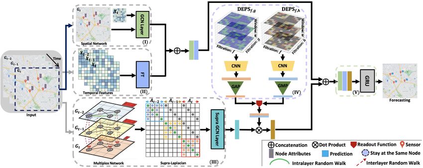
Figure 1: TAMP-S2GCNets consists of 5 components: (I) Spatial graph convolutional layer on Gt
extracts spatial information at time t (see Eq. 5). (II) Feature transformation (FT) learns representa-
tion of the spatio-temporal data X T over a sliding window of size T (see Eq. 1). (III) Supragraph
convolutional module captures joint spatio-temporal dependencies in X T (see Eq. 4). (IV) Detailed
architecture of the DEPSRL module (see Eqs. 6 and 7), where the DEPS with different types of mul-
tifiltrations can be learned by a CNN base model and global pooling mechanism. Here DEPS allows
us to learn the intrinsic graph structure both across multiple geometric dimensions and across time.
(V) The learned spatio-temporal dependencies are passed into GRU layer (see Eq. 8) for multi-step
forecasting. Note that the whole model can be trained in an end-to-end fashion.
5 E XPERIMENTS
Data Description We use three different types of datasets to examine the performance of the pro-
posed TAMP-S2GCNets on dynamic networks: (i) The transportation and traffic data of California
state from the freeway Performance Measurement System (PeMS). We use three well-studied traffic
networks from literature: PeMSD3, PeMSD4 and PeMSD8 (Chen et al., 2001), (ii) Digital transac-
tions between users in the Ethereum blockchain network. We extract dynamic networks from three
token assets: Bytom, Decentraland and Golem (Li et al., 2020), and (iii) The spread of coronavirus
disease COVID-19 at county-level in states of California (CA) and Texas (TX). More details on each
dataset and parameter settings are provided in Appendix D.1.
Experimental Settings We compare the presented TAMP-S2GCNets with 13 state-of-the-art base-
lines (see more details of baselines in Appendix D.2) on three evaluation metrics, i.e, Mean Absolute
Error (MAE), Root Mean Squared Error (RMSE), and Mean Absolute Percentage Error (MAPE).
For transportation networks, following Cao et al. (2020), we (i) split PeMSD3, PeMSD4, and
PeMSD8 datasets into a training set (60%), validation set (20%), and test set (20%) in chronologi-
cal order and (ii) use the one hour historical data to the next 15 minutes data. Following Chen et al.
(2021), we (i) split Bytom, Decentraland, and Golem token networks into training set (80%) and test
set (20%) in chronological order and (ii) use 7 days historical data to predict future 7 days data. For
COVID-19 datasets, in our experiments, we use daily data of 11 months of 2020, from February 1 to
December 31, and split the graph signals into training set, first 80% of days (268 days), and test set,
last 20% of days (67 days). Further specifics on experimental setup are provided in Appendix D.2.
The best results are in bold font and the results with dotted underline are the best performance
achieved by the runner-ups. We also perform a one-sided two-sample t-test between the best result
and the best performance achieved by the runner-up, where *, **, *** denote significant, statisti-
cally significant, highly statistically significant results, respectively. More detailed experiments on
all datasets are in Appendix E. The data and code implementation are available at https://www.
dropbox.com/sh/n0ajd5l0tdeyb80/AABGn-ejfV1YtRwjf_L0AOsNa?dl=0.
Computational Complexity Although, in general, MP is computationally costly, in our case, to
get the DEPS summary, we do not need to compute PDs as in other MP approaches, but only
Betti numbers of each filtration cell. In particular, while a computational cost for obtaining k th -
PD for a graph is O(M3k ), where Mk is the number k-simplices (Otter et al., 2017), obtaining
Euler Characteristics by sparse matrix methods has computational complexity of O(M0 + M1 +
M2 ) (Edelsbrunner & Parsa, 2014).
7Under review as a conference paper at ICLR 2022
5.1 E XPERIMENTAL R ESULTS
Transportation Traffic Flow Table 1 shows the performance comparison among 13 state-of-the-art
baselines on PeMSD3, PeMSD4, and PeMSD8 for multi-step traffic flow forecasting. Our TAMP-
S2GCNets consistently outperforms baseline models on all 3 datasets except for PeMSD3, which
underscore effectiveness of TAMP-S2GCNets in time series forecasting tasks. On PeMSD3, our
TAMP-S2GCNets achieves the best MAE and MAPE, and has an average 2.75% relative gain, com-
pared to the runner-up. The average relative gains of TAMP-S2GCNets over the runner-ups in MAE
and MAPE are 2.78% and 2.19% on the 3 datasets, respectively.
Ethereum Blockchain Prices Table 3 (left) summarizes the comparison results in MAPE on 3
Ethereum token networks (i.e., Bytom, Decentrland, and Golen). Table 3 indicates that TAMP-
S2GCNets is always better than baselines for all dynamic Ethereum networks. We find that, even
compared to the baseline which also integrates topological information (i.e., Z-GCNETs), TAMP-
S2GCNets is highly competitive, implying that the time-aware MP representation with DEPS is
capable of better encoding time-conditioned information than the zigzag idea based on one filtration.
COVID-19 Hospitalizations Table 2 shows results on 15-day ahead forecasting of COVID-19 hos-
pitalizations in the U.S. states of California (CA) and Texas (TX) at a county level basis (RMSE
is aggregated over each state). For the sake of room, here we only display the top runner models.
TAMP-S2GCNets yields significantly better forecasting performance, with relative gains of 1.5%-
24.5% (in CA) and 5.5%-46.7% (in TX).
Table 1: Forecasting performance on PeMSD3, PeMSD4 and PeMSD8, along with results on sta-
tistical significance. Standard deviations are suppressed for the sake of room and are reported in
Table 8 in Appendix E.
PeMSD3 PeMSD4 PeMSD8
Model
MAE RMSE MAPE (%) MAE RMSE MAPE (%) MAE RMSE MAPE (%)
FC-LSTM (Sutskever et al., 2014) 21.33 35.11 23.33 27.14 41.59 18.20 22.20 34.06 14.20
SFM (Zhang et al., 2017) 17.67 30.01 18.33 24.36 37.10 17.20 16.01 27.41 10.40
N-BEATS (Oreshkin et al., 2019) 18.45 31.23 18.35 25.56 39.90 17.18 19.48 28.32 13.50
DCRNN (Li et al., 2018) 18.18 30.31 18.91 24.70 38.12 17.12 17.86 27.83 11.45
LSTNet (Lai et al., 2018) 19.07 29.67 17.73 24.04 37.38 17.01 20.26 31.96 11.30
STGCN (Yu et al., 2018) 17.49 30.12 17.15 22.70 35.50 14.59 18.02 27.83 11.40
TCN (Bai et al., 2018) 18.23 25.04 19.44 26.31 36.11 15.62 15.93 25.69 16.50
∗
DeepState (Rangapuram et al., 2018) 15.59 20.21 18.69 26.50 33.00 15.40 19.34 27.18 16.00
GraphWaveNet (Wu et al., 2019) 19.85 32.94 19.31 26.85 39.70 17.29 19.13 28.16 12.68
DeepGLO (Sen et al., 2019) 17.25 23.25 19.27 25.45 35.90 12.20 15.12 25.22 13.20
AGCRN (Bai et al., 2020) 14.22 24.03 13.89 17.78
...... 29.17 11.79
. . . . . . . 14.59 23.06 9.29
Z-GCNETs (Chen et al., 2021) 14.20
...... 25.29 13.88
...... 18.05 29.08
...... 11.79
. . . . . . . 14.52
...... 23.00
...... 9.28
StemGNN (Cao et al., 2020) 14.32 21.64
...... 16.24 20.20 31.83 12.00 15.83 24.93 9.26
.....
∗∗ ∗ ∗∗
TAMP-S2GCNets (ours) 13.91 23.77 13.40 17.58 28.56 11.01 13.77 21.70 8.99
5.2 A BLATION S TUDIES
Contribution of TAMP-S2GCNets components We now conduct the ablation stud-
ies on PeMSD4 and PeMSD8 to evaluate contribution of different components of our
framework. (Ablation results on Golem and CA are in Table 9 in Appendix E.)
We compare our TAMP-S2GCNets with 4 Table 2: 15-day ahead forecasting results (RMSE) on
ablated variants, i.e., (i) TAMP-S2GCNets COVID-19 hospitalizations in CA and TX.
without DEPSRL module (w/o DEPSRL
module), (ii) TAMP-S2GCNets without
spatial graph convolutional layer (w/o Model CA TX
GCNSpa ), (iii) TAMP-S2GCNets with- DCRNN (Li et al., 2018) 492.10±2.96 90.47±2.28
out supragraph convolutional module (w/o AGCRN (Bai et al., 2020) 448.27±2.78 52.96±3.92
GCNSup ), and (iv) TAMP-S2GCNets with- StemGNN (Cao et al., 2020) ...............
377.25±3.91 ..............
51.00±2.60
out FT (w/o FT). As Table 3 (right panel) TAMP-S2GCNets (ours) ∗ 371.60±2.68 ∗ 48.21±3.17
shows, ablating each of above causes the
performance drops sharply in comparison with our full TAMP-S2GCNets model. Especially, on
PeMSD4, the supragraph convolutional module significantly improves the results as it simultane-
ously captures the spatial and temporal information. In addition, it is evident that DEPSRL mod-
8Under review as a conference paper at ICLR 2022
ule enhances the topological information learning ability in spatio-temporal domain, i.e., TAMP-
S2GCNets outperforms TAMP-S2GCNets w/o DEPSRL module with an average relative gain
3.92% on RMSE over PeMSD4 and PeMSD8. Besides, as expected, taking the advantages of
GCNSpa and FT, we improve the performance via capturing the graph structure in the spatial di-
mension and consolidating the processing of spatio-temporal correlations between node attributes,
respectively.
Table 3: Forecasting performance (MAPE in %) on Ethereum networks (left panel) and the TAMP-
S2GCNets ablation study on PeMSD4 and PeMSD8 (right panel).
Model Bytom Decentraland Golem Architecture MAE RMSE MAPE
TAMP-S2GCNets 17.58 28.56 11.01
DCRNN (Li et al., 2018) 35.36±1.18 27.69±1.77 23.15±1.91 W/o DEPSRL 17.89 ∗∗∗
29.99 ∗
11.07
∗∗ ∗∗∗ ∗∗∗
STGCN (Yu et al., 2018) 37.33±1.06 28.22±1.69 23.68±2.31 PeMSD4 W/o GCNSpa 19.41 30.90 11.21
∗∗∗ ∗∗∗ ∗∗∗
GraphWaveNet (Wu et al., 2019) 39.18±0.96 37.67±1.76 28.89±2.34 W/o GCNSup 20.61 31.82 12.64
∗ ∗∗∗ ∗∗∗
W/o FT 18.30 29.65 12.29
AGCRN (Bai et al., 2020) 34.46±1.37 26.75±1.51 22.83±1.91
TAMP-S2GCNets 13.77 21.70 8.99
Z-GCNETs (Chen et al., 2021) 31.04±0.78
... ... .. .. ... . 23.81±2.43
.. .. .. . . . . . . . . 22.32±1.42
............. W/o DEPSRL ∗∗∗
14.28 ∗∗
22.39 9.32
∗∗
StemGNN (Cao et al., 2020) 34.91±1.04 28.37±1.96 22.50±2.01 PeMSD8 W/o GCNSpa 14.16 22.29 9.40
∗
W/o GCNSup 13.99 21.91 9.07
∗ ∗∗∗ ∗∗ ∗∗∗ ∗∗∗
TAMP-S2GCNets (ours) 29.26±1.06 19.89±1.49 20.10±2.30 W/o FT 14.36 22.60 9.26
Table 4: MAPE (%) (standard deviation) of TAMP-S2GCNets with single- and multifiltrations
(left panel) and MAPE (%) and computation time for TAMP-S2GCNets with our DEPS, MP-I
of Carrière & Blumberg (2020) and MP-L of Vipond (2020) (right panel).
TAMP-S2GCNets on Bytom (Left) TAMP-S2GCNets on Bytom (Right)
Single filtration Multifiltration MP summary MAPE (%) Running time (s)
- Deg & Btwns: 30.02±1.05 MP-I (Carrière & Blumberg, 2020) 33.13 401.80
Deg: 30.56±1.08 Btwns & PowerTrns : 29.26±0.96 MP-L (Vipond, 2020) 32.19 517.11
Btwns: 30.80±1.70 Btwns & PowerVol : .29.27±0.78
............. DEPSDeg & Btwns 30.02 47.67
PowerTrns : 31.04±1.90 Deg & PowerTrns : 29.86±1.05 DEPSDeg & PowerTrns 29.86
...... 39.46
......
PowerVol : 30.79±1.61 Deg & PowerVol : 29.41±1.06 DEPSBtwns & PowerTrns 29.26 29.84
Contribution of Single vs. Multifiltration Persistence We consider sublevel filtrations based on
node degree (Deg), betweenness (Btwns), and graph diameter (power filtration) with edge weights
induced by number of transactions (PowerTrns ) and volume of transactions (PowerVol ). As Table 4
(left) shows, MP always outperforms single filtrations by a significant margin, both in terms of
prediction accuracy and variability. The results confirm our premise that MP is able (i) to capture
hidden time dependencies of high dimensional time-varying objects which are inaccessible with
one-parameter PH and (ii) to yield substantially more stable feature maps in dynamic scenarios.
Contribution of DEPS vs. the Existing MP Summaries Finally, we evaluate performance of the
new time-aware MP summary, i.e., DEPS, in comparison to the MP summaries based on the slic-
ing argument, namely, MP-I of Carrière & Blumberg (2020) and MP-L of Vipond (2020) as rep-
resentation input to TAMP-S2GCNets. As Table 4 (right panel) shows, comparing to MP-I and
MP-L, DEPS yields 9%-12% improvement in MAPE, and at least a 10 times decrease in com-
putational time (29.84s for DEPS vs. 401.80s for MP-I and 517.11s for MP-L). Such substantial
differences in computational costs are explained by the need of the slicing-based MP summaries to
search for the most suitable one-parameter PH representation of MP. In turn, DEPS is based on a
point-wise representation argument in linear algebra, and its high computational efficiency makes
DEPS the preferred choice for time-conditioned topological representation learning (see the running
time in Table 4). Since computational costs remain the major roadblock for MP applications, our
DEPS approach shows that MP tools based on scalable sparse matrix algorithms appear to be the
most promising direction for integration of MP into machine learning tasks.
6 C ONCLUSION
We have explored utility of MP to enhance knowledge representation mechanisms within the time-
aware DL paradigm. The developed TAMP-S2GCNets model is shown to yield highly competitive
forecasting performance on a wide range of datasets, with much lower computational costs. In
the future we plan to explore combination of MP with the zigzag persistence and to investigate
asymptotic distributional properties of point-wise MP invariants.
9Under review as a conference paper at ICLR 2022
E THICS S TATEMENT
We do not anticipate any negative ethical implications of the proposed methodology. In turn, we
believe that introduction of GCNs tools, coupled with multiparameter topological approaches, into
biosurveillance opens a new path for more accurate, timely, and robust tracking of infectious dis-
eases with high virulence such as COVID-19. In particular, multiparameter persistence allows for
extracting the most salient topological features along multiple geometric dimensions and, as such,
can be especially valuable to address disease dynamics as a function of multiple highly heteroge-
neous variables, e.g., socio-demographic, socio-environmental, and socio-economic factors. In turn,
GCNs and, more generally, geometric deep learning allow for capturing sophisticated nonlinear
spatio-temporal dependencies among factors which contribute to the disease spread. Hence, we pos-
tulate that in the next few years we can expect to see a new set of spatio-temporal biosurveillance
artificial intelligence algorithms, based on a combination of geometric deep learning, multiparame-
ter persistence, and more generally, tools of topological data analysis.
R EPRODUCIBILITY S TATEMENT
To support reproducibility of the results in the paper, we have submitted our datasets and codes
(see https://www.dropbox.com/sh/n0ajd5l0tdeyb80/AABGn-ejfV1YtRwjf_
L0AOsNa?dl=0) as the supplementary information.
R EFERENCES
U.S. Census Bureau: county adjacency file record layout. https://www.census.
gov/programs-surveys/geography/technical-documentation/
records-layout/county-adjacency-record-layout.html, a. Accessed:
2021-05-26.
U.S. Census Bureau: county population totals and components of change. https:
//www.census.gov/data/datasets/time-series/demo/popest/
2010s-counties-total.html, b. Accessed: 2021-05-26.
CovidActNow: u.s. covid risk & vaccine tracker. https://covidactnow.org, c. Accessed:
2021-05-26.
Etherscan: block explorer and analytics platform for ethereum, a decentralized smart contracts plat-
form. https://etherscan.io, d. Accessed: 2021-05-26.
Ethereum: community-run technology powering the cryptocurrency ether (ETH) and thousands of
decentralized applications. https://ethereum.org, e. Accessed: 2021-05-26.
JHU: covid-19 data from the johns hopkins university. https://github.com/
CSSEGISandData/COVID-19, f. Accessed: 2021-05-26.
Henry Adams, Tegan Emerson, Michael Kirby, Rachel Neville, Chris Peterson, Patrick Shipman,
Sofya Chepushtanova, Eric Hanson, Francis Motta, and Lori Ziegelmeier. Persistence images: A
stable vector representation of persistent homology. Journal of Machine Learning Research, 18
(8):1–35, 2017. URL http://jmlr.org/papers/v18/16-337.html.
Robert J Adler, Omer Bobrowski, Matthew S Borman, Eliran Subag, Shmuel Weinberger, et al.
Persistent homology for random fields and complexes. In Borrowing strength: theory powering
applications–a Festschrift for Lawrence D. Brown, pp. 124–143. 2010.
Lei Bai, Lina Yao, Can Li, Xianzhi Wang, and Can Wang. Adaptive graph convolutional recurrent
network for traffic forecasting. Advances in Neural Information Processing Systems, 33, 2020.
Shaojie Bai, J Zico Kolter, and Vladlen Koltun. An empirical evaluation of generic convolutional
and recurrent networks for sequence modeling. arXiv preprint arXiv:1803.01271, 2018.
Yuliy Baryshnikov and Robert Ghrist. Euler integration over definable functions. Proceedings of
the National Academy of Sciences, 107(21):9525–9530, 2010.
10Under review as a conference paper at ICLR 2022
Gabriele Beltramo, Rayna Andreeva, Ylenia Giarratano, Miguel O Bernabeu, Rik Sarkar, and Pri-
moz Skraba. Euler characteristic surfaces. arXiv:2102.08260, 2021.
Chen Cai and Yusu Wang. Understanding the power of persistence pairing via permutation test.
arXiv preprint arXiv:2001.06058, 2020.
Defu Cao, Yujing Wang, Juanyong Duan, Ce Zhang, Xia Zhu, Congrui Huang, Yunhai Tong, Bix-
iong Xu, Jing Bai, Jie Tong, and Qi Zhang. Spectral temporal graph neural network for multivari-
ate time-series forecasting. In Advances in Neural Information Processing Systems, volume 33,
pp. 17766–17778, 2020.
Gunnar Carlsson and Rickard Brüel Gabrielsson. Topological approaches to deep learning. In
Topological Data Analysis, pp. 119–146. Springer, 2020.
Gunnar Carlsson and Afra Zomorodian. The theory of multidimensional persistence. Discrete &
Computational Geometry, 42(1):71–93, 2009.
Mathieu Carrière and Andrew Blumberg. Multiparameter persistence image for topological machine
learning. Advances in Neural Information Processing Systems, 33, 2020.
Mathieu Carrière, Frédéric Chazal, Yuichi Ike, Théo Lacombe, Martin Royer, and Yuhei Umeda.
Perslay: A neural network layer for persistence diagrams and new graph topological signatures.
In AISTATS, pp. 2786–2796, 2020.
Andrea Cerri, Barbara Di Fabio, Massimo Ferri, Patrizio Frosini, and Claudia Landi. Betti num-
bers in multidimensional persistent homology are stable functions. Mathematical Methods in the
Applied Sciences, 36(12):1543–1557, 2013.
Chao Chen, Karl Petty, Alexander Skabardonis, Pravin Varaiya, and Zhanfeng Jia. Freeway perfor-
mance measurement system: mining loop detector data. Transportation Research Record, 1748
(1):96–102, 2001.
Yuzhou Chen, Ignacio Segovia-Dominguez, and Yulia R Gel. Z-gcnets: Time zigzags at graph con-
volutional networks for time series forecasting. International Conference on Machine Learning,
2021.
David Cohen-Steiner, Herbert Edelsbrunner, and John Harer. Stability of persistence diagrams.
Discrete & computational geometry, 37(1):103–120, 2007.
René Corbet, Ulderico Fugacci, Michael Kerber, Claudia Landi, and Bei Wang. A kernel for multi-
parameter persistent homology. Computers & graphics: X, 2:100005, 2019.
Baris Coskunuzer, Cuneyt Gurcan Akcora, Ignacio Segovia Dominguez, Zhiwei Zhen, Murat
Kantarcioglu, and Yulia R Gel. Smart vectorizations for single and multiparameter persistence.
arXiv:2104.04787, 2021.
M. di Angelo and G. Salzer. Tokens, types, and standards: Identification and utilization in
ethereum. In 2020 IEEE International Conference on Decentralized Applications and Infras-
tructures (DAPPS), pp. 1–10, 2020. doi: 10.1109/DAPPS49028.2020.00001.
Ensheng Dong, Hongru Du, and Lauren Gardner. An interactive web-based dashboard to track
covid-19 in real time. The Lancet Infectious Diseases, 20(5), May 2020. doi: 10.1016/
S1473-3099(20)30120-1.
Herbert Edelsbrunner and John Harer. Computational topology: an introduction. American Mathe-
matical Soc., 2010.
Herbert Edelsbrunner and Salman Parsa. On the computational complexity of betti numbers: re-
ductions from matrix rank. In Proceedings of the twenty-fifth annual ACM-SIAM symposium on
discrete algorithms, pp. 152–160. SIAM, 2014.
Robert Ghrist. Homological algebra and data. Math. Data, 25:273, 2018.
Allen Hatcher. Algebraic Topology. Cambridge University Press, 2002.
11Under review as a conference paper at ICLR 2022
Christoph Hofer, Florian Graf, Bastian Rieck, Marc Niethammer, and Roland Kwitt. Graph filtration
learning. In International Conference on Machine Learning, pp. 4314–4323. PMLR, 2020.
Christoph D Hofer, Roland Kwitt, and Marc Niethammer. Learning representations of persistence
barcodes. JMLR, 20(126):1–45, 2019.
Max Horn, Edward De Brouwer, Michael Moor, Yves Moreau, Bastian Rieck, and Karsten Borg-
wardt. Topological graph neural networks. arXiv:2102.07835, 2021.
Michael Kerber. Multi-parameter persistent homology is practical. 2020.
Michael Kerber and Alexander Rolle. Fast minimal presentations of bi-graded persistence modules.
In 2021 Proceedings of the Workshop on Algorithm Engineering and Experiments (ALENEX), pp.
207–220. SIAM, 2021.
Guokun Lai, Wei-Cheng Chang, Yiming Yang, and Hanxiao Liu. Modeling long-and short-term
temporal patterns with deep neural networks. In The 41st International ACM SIGIR Conference
on Research & Development in Information Retrieval, pp. 95–104, 2018.
Claudia Landi. The rank invariant stability via interleavings. arXiv:1412.3374, 2014.
Michael Lesnick and Matthew Wright. Computing minimal presentations and bigraded betti num-
bers of 2-parameter persistent homology. arXiv preprint arXiv:1902.05708, 2019.
Yaguang Li, Rose Yu, Cyrus Shahabi, and Yan Liu. Diffusion convolutional recurrent neural net-
work: Data-driven traffic forecasting. In International Conference on Learning Representations,
2018.
Yitao Li, Umar Islambekov, Cuneyt Akcora, Ekaterina Smirnova, Yulia R. Gel, and Murat Kantar-
cioglu. Dissecting ethereum blockchain analytics: What we learn from topology and geometry of
the ethereum graph? In Proceedings of the 2020 SIAM International Conference on Data Mining,
SDM 2020, pp. 523–531, 2020.
Boris N Oreshkin, Dmitri Carpov, Nicolas Chapados, and Yoshua Bengio. N-beats: Neural ba-
sis expansion analysis for interpretable time series forecasting. In International Conference on
Learning Representations, 2019.
Nina Otter, Mason A Porter, Ulrike Tillmann, Peter Grindrod, and Heather A Harrington. A roadmap
for the computation of persistent homology. EPJ Data Science, 6:1–38, 2017.
Syama Sundar Rangapuram, Matthias W Seeger, Jan Gasthaus, Lorenzo Stella, Yuyang Wang, and
Tim Januschowski. Deep state space models for time series forecasting. Advances in neural
information processing systems, 31:7785–7794, 2018.
Hans Riess and Jakob Hansen. Multidimensional persistence module classification via lattice-
theoretic convolutions. 2020.
Rajat Sen, Hsiang-Fu Yu, and Inderjit S Dhillon. Think globally, act locally: A deep neural net-
work approach to high-dimensional time series forecasting. In Advances in Neural Information
Processing Systems, volume 32, 2019.
Ilya Sutskever, Oriol Vinyals, and Quoc V Le. Sequence to sequence learning with neural networks.
In Advances in Neural Information Processing Systems, volume 27, 2014.
Ashleigh Linnea Thomas. Invariants and Metrics for Multiparameter Persistent Homology. PhD
thesis, Duke University, 2019.
Gugan C Thoppe, D Yogeshwaran, Robert J Adler, et al. On the evolution of topology in dynamic
clique complexes. Advances in Applied Probability, 48(4):989–1014, 2016.
Virginia Vassilevska, Ryan Williams, and Raphael Yuster. Finding the smallest h-subgraph in real
weighted graphs and related problems. In Automata, Languages and Programming, pp. 262–273.
Springer Berlin Heidelberg, 2006.
Oliver Vipond. Multiparameter persistence landscapes. Journal of Machine Learning Research, 21
(61):1–38, 2020.
12Under review as a conference paper at ICLR 2022
Matthew Wright and Xiaojun Zheng. Topological data analysis on simple english wikipedia articles.
arXiv:2007.00063, 2020.
Zonghan Wu, Shirui Pan, Guodong Long, Jing Jiang, and Chengqi Zhang. Graph wavenet for deep
spatial-temporal graph modeling. In Proceedings of the 28th International Joint Conference on
Artificial Intelligence, 2019.
Huaxiu Yao, Fei Wu, Jintao Ke, Xianfeng Tang, Yitian Jia, Siyu Lu, Pinghua Gong, Jieping Ye, and
Zhenhui Li. Deep multi-view spatial-temporal network for taxi demand prediction. In Proceed-
ings of the AAAI Conference on Artificial Intelligence, volume 32, 2018.
Bing Yu, Haoteng Yin, and Zhanxing Zhu. Spatio-temporal graph convolutional networks: a deep
learning framework for traffic forecasting. In Proceedings of the 27th International Joint Confer-
ence on Artificial Intelligence, pp. 3634–3640, 2018.
Liheng Zhang, Charu Aggarwal, and Guo-Jun Qi. Stock price prediction via discovering multi-
frequency trading patterns. In Proceedings of the 23rd ACM SIGKDD international conference
on knowledge discovery and data mining, pp. 2141–2149, 2017.
13Under review as a conference paper at ICLR 2022
A N OTATION
Frequently used notation is summarized in Table 5.
Table 5: The main symbols and definitions in this paper.
Notation Definition
Gt the spatial network at timestamp t
N the number of nodes
Mt the number of edges at timestamp t
X a sequence of observations on a multivariate variable
Xt node feature matrix at timestamp t
C simplicial complex
f filtering function for sublevel filtration
Mk number of k-simplices
Dk (C) k-dimensional persistence diagram
χ(C) Euler-Poincaré Characteristics
Hk (C) k th homology group
F (·, ·) multivariate filtering function
E± Euler-Poincaré Surfaces
{Et }Tt=1 Dynamic Euler-Poincaré Surface
(Σ, A, P) a probability space
F a filtration of σ-fields
W1 Wasserstein-1 distance
D(·, ·) the distance function for MP
B(·) the Betti function
Mk the number k-simplices
FN the feature dimension
T the sliding window size
F(·) the multivariate forecasting model
S the normalized self-adaptive adjacency matrix
Eφ the learnable node embedding
S̃ Laplacian tensor
K the length of Laplacian tensor S̃
L supra-Laplacian
Φ the output of DEPSRL module
F (·, ·, ·) the dimension-wise concatenation function
B S INGLE PARAMETER P ERSISTENT H OMOLOGY AND I TS S UMMARIES
All extracted topological features can be then summarized as a multiset in R2 , called persistence
diagram (PD): Dk (C) = {(bi , di ) ∈ R2 | bi < di }, where birth bi and death di mark the filtration
indexes at which the k-dimensional topological feature ρi appears and disappears, respectively. The
farther (bi , di ) from the diagonal is (that is, the more persistent ρi is), the likelier ρi is to contain
salient information on Gt . Multiplicity of (xb , yd ) ∈ D is the number of p-dimensional topological
features (p-holes) that are born and die at xb and yb , respectively. Features on the diagonal of D
have infinite multiplicity.
Another summary which may be particularly suitable in our context of modeling noisy time-evolving
objects is the Euler-Poincaré Characteristics (see Adler et al. (2010); Baryshnikov & Ghrist (2010)
on the Euler calculus and its applications, particular, in conjunction with sensor networks).
Definition B.1 (Euler-Poincaré Characteristics). For a given simplicial complex C, Euler-Poincaré
Characteristics χ(C) is defined as the alternating sum of the number of k-simplices of C. That is, if
PM
nk is the number of k-simplices in C, then χ(C) = k=0 (−1)k nk , where M is the dimension of
highest dimensional simplex in C. Note that Euler-Poincaré Characteristics is homotopy invariant,
14Under review as a conference paper at ICLR 2022
PM
and an alternative definition is χ(C) = k=0 (−1)k Bk (C) where Bk (C) is the k th Betti number
of C, i.e. rank of the k th homology group Hk (C) (Ghrist, 2018; Hatcher, 2002).
C P ROOF OF T HEOREM 3.1
In this section, we provide the proof of the stability theorem (Theorem 3.1). First, let us recall the
key notations we use. Let G + and G − be two graphs and let C± be the clique complexes of G ±
(Ghrist, 2018). Let F = (f, g) be a multivariate filter function, i.e. F : V ± → R2 , where V ± is the
set of nodes of G ± , and let I = {(αi , βj ) | 1 ≤ i ≤ m, 1 ≤ j ≤ n} be the corresponding thresholds
for F = (f, g).
Next, we define Wasserstein-p distance among PDs, i.e., the important concept we borrow from the
theory of single parameter persistence (Edelsbrunner & Harer, 2010).
Definition C.1 (Wasserstein-p distance). Let (C± , f ± , I ± ) be two single parameter filtrations, and
Dk (C± ) be the corresponding PDs for k-cycles (i.e, k-dimensional topological features). Let qj+ =
(b+ + +
j , dj ) ∈ Dk (C ) be the birth and death times of a k-dimensional topological feature ρj . Then,
Wasserstein-p distance between Dk (C+ ) and Dk (C− ) is defined as
X p1
−
+
Wp (Dk (C ), Dk (C )) = inf kqj+ − φ(qj+ )kp∞ , p ∈ Z+ , (9)
φ
j∈D(C+ )∪∆
where φ : Dk (C+ ) ∪ ∆ → Dk (C− ) ∪ ∆ is a bijection (matching) and ∆ is the diagonal set, i.e.,
∆ = {(b, b)|b ∈ R}, which contains k-cycles of infinite multiplicity. With ∆ in both sides, we
ensure the existence of these bijections even if the cardinalities |{qj+ }| and |{ql− }| are different.
When p = ∞, (9) corresponds to the bottleneck distance, i.e. W∞ . In the proof below, we use
p = 1, i.e. W1 -distance.
Armed the PD and Wasserstein-p distance concepts, we now turn to the main stability result for the
new MP summary. Let C b ± = {C± } be the bifiltration associated with (C± , F, I), i.e. C± is the
ij ij
±
clique complex of the induced subgraph Gij = F −1 ((−∞, αi ] × (−∞, βj ]). (Figure 2 illustrates
such bifiltration on graphs with degree and eccentricity functions.) Let E± be the the corresponding
Euler-Poincaré Surface, i.e. E± is an m × n-matrix with entries E± ±
ij = χ(Cij , ), where χ(.) is
+ −
the Euler Characteristics (See Figure 2), and D(C , C ) be the weak L1 -distance as defined in
Section 3 of the paper (see also Remark C.1 below for the motivation to use this new metric).
Proof of Theorem 3.1: We start from providing the outline of the proof. Notice that Euler-Poincaré
Surfaces is the alternating sum of Betti numbers {Bk }. Hence, the distance kE+ −E− k1,1 is bounded
by the difference of the corresponding Betti numbers for C b ± , i.e. Eqs. (10) and (11). By fixing i
and k, and by taking column distance Dc into consideration, our main assertion
kE+ − E− k1,1 ≤ C · D(C b − ),
b +, C C>0
−
then reduces to Eqs. (12) and (13). To relate the difference |B(C+ j ) − B(Cj )| to
+ − ±
W1 (D(C ), D(C )), we observe that the Betti number B(Cj ) is the sum of the number of bar-
codes in D(C± ), containing βj , i.e., #{r | βj ∈ [b± ±
r , dr )} (Eqs. (13) and (14)). Yet, the differences
of the number of barcodes containing βj for C+ and C− can be bounded by the Wasserstein-1 dis-
tances of D(C+ ) and D(C− ), i.e. Eqs. (15) and (16). Aggregating these terms on indices i and k
finishes the proof.
PM k
Now, we turn to derivations in details. Recall that χ(C) = k=0 (−1) Bk (C), where Bk (C)
th
is the k Betti number of C and M is the maximum homological dimension of C. Then, since
PM
E± ± ±
ij = χ(Cij ), we have Eij =
±
k=0 Bk (Cij ). Hence, for any i, j,
M
X M
X
− − −
|E+
ij − Eij | = | (−1)k [Bk (C+
ij ) − Bk (Cij )]| ≤ |Bk (C+
ij ) − Bk (Cij )|. (10)
k=0 k=0
15You can also read