Reengineering and optimization of GEOtop software package - MASTER IN HIGH PERFORMANCE COMPUTING
←
→
Page content transcription
If your browser does not render page correctly, please read the page content below
M ASTER IN H IGH P ERFORMANCE
              C OMPUTING

Reengineering and optimization of
    GEOtop software package

 Supervisors:
 Giacomo B ERTOLDI,
 Alberto S ARTORI,
 Stefano C OZZINI

                                         Candidate:
                                    Elisa B ORTOLI

                      4th EDITION
                      2017–2018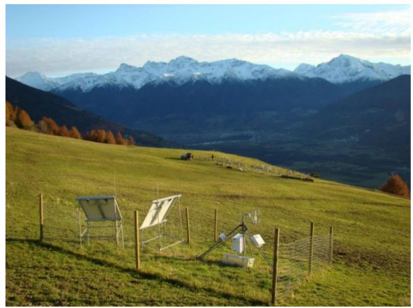
i

                   Acknowledgements
The research reported in this work was supported by OGS, CINECA and
EURAC Research under HPC-TRES program award number 2017-20.

The computational results presented have been achieved [in part] using the
Vienna Scientific Cluster (VSC).

For the test cases, data from the Long Term Ecological Research Area Mazia
Valley (South Tyrol, Italy) have been used.

Giacomo Bertoldi, Alberto Sartori and Stefano Cozzini are acknowledged for
the thesis supervision.

Siegfried Höfinger, Samuel Senorer, Martin Palma, Luca Cattani, Christian
Brida and Emanuele Cordano are acknowledged for their technical support.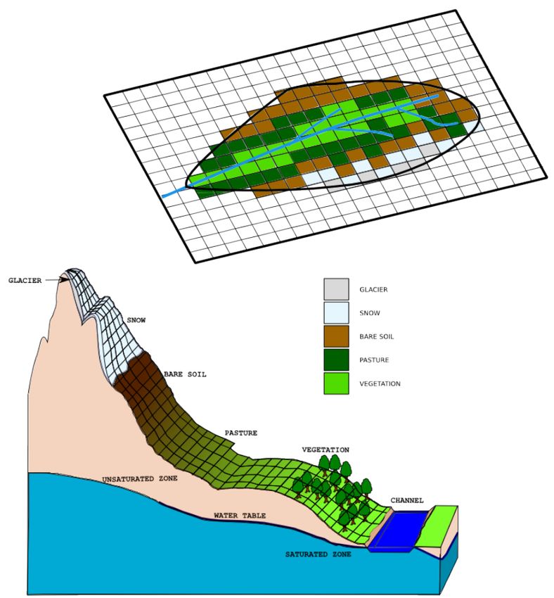
iii

Contents

Acknowledgements                                                                                                                i

1   Introduction                                                                                                                1

2   Model overview                                                                                                              3
    2.1 Landscape and equation discretization                          .   .   .   .   .   .   .   .   .   .   .   .   .   .    3
    2.2 Water and energy budgets . . . . . . .                         .   .   .   .   .   .   .   .   .   .   .   .   .   .    3
    2.3 Numerics . . . . . . . . . . . . . . . . .                     .   .   .   .   .   .   .   .   .   .   .   .   .   .    5
    2.4 Software package . . . . . . . . . . . .                       .   .   .   .   .   .   .   .   .   .   .   .   .   .    7
        2.4.1 Simulation flow chart . . . . .                          .   .   .   .   .   .   .   .   .   .   .   .   .   .    7
        2.4.2 Simulation types . . . . . . . .                         .   .   .   .   .   .   .   .   .   .   .   .   .   .    9

3   GEOtop 3.0                                                                                                                 11
    3.1 Background . . . . . . . .         .   .   .   .   .   .   .   .   .   .   .   .   .   .   .   .   .   .   .   .   .   11
    3.2 Easy to compile and run .          .   .   .   .   .   .   .   .   .   .   .   .   .   .   .   .   .   .   .   .   .   12
    3.3 Modular and flexible . . .         .   .   .   .   .   .   .   .   .   .   .   .   .   .   .   .   .   .   .   .   .   12
    3.4 Tested as much as possible         .   .   .   .   .   .   .   .   .   .   .   .   .   .   .   .   .   .   .   .   .   15
    3.5 Computationally efficient          .   .   .   .   .   .   .   .   .   .   .   .   .   .   .   .   .   .   .   .   .   18

4   Test cases                                                                                                                 21
    4.1 Matsch_B2_Ref_007 . . . . . . . . . . . . . . . . . . . . . . . . .                                                    22
    4.2 snow_dstr_SENSITIVITY . . . . . . . . . . . . . . . . . . . . .                                                        23
    4.3 Muntatschini_ref_005 . . . . . . . . . . . . . . . . . . . . . . . .                                                   24

5   Used architectures                                                                                                         25
    5.1 Local pc . . . . . . . . . . . . . . . . . . . . . . . . . . . . . . . .                                               25
    5.2 VSC-3 . . . . . . . . . . . . . . . . . . . . . . . . . . . . . . . . .                                                26

6   Profiling                                                                                                                  27
    6.1 Likwid-perfctr . . . . . . . . . . . . . . . . . . . . . . . . . . . .                                                 27
    6.2 Callgrind . . . . . . . . . . . . . . . . . . . . . . . . . . . . . . .                                                31
    6.3 Class Timer . . . . . . . . . . . . . . . . . . . . . . . . . . . . .                                                  39

7   Optimizations                                                                                                              43
    7.1 Maths optimization . . .       .   .   .   .   .   .   .   .   .   .   .   .   .   .   .   .   .   .   .   .   .   .   43
    7.2 OpenMP parallelization         .   .   .   .   .   .   .   .   .   .   .   .   .   .   .   .   .   .   .   .   .   .   44
    7.3 Automatic vectorization        .   .   .   .   .   .   .   .   .   .   .   .   .   .   .   .   .   .   .   .   .   .   46
    7.4 Combination . . . . . . .      .   .   .   .   .   .   .   .   .   .   .   .   .   .   .   .   .   .   .   .   .   .   46
iv

8    Optimization results                                                                                                      47
     8.1 Default 3.0 . . . . . . . .   .   .   .   .   .   .   .   .   .   .   .   .   .   .   .   .   .   .   .   .   .   .   47
     8.2 Maths optimization . . .      .   .   .   .   .   .   .   .   .   .   .   .   .   .   .   .   .   .   .   .   .   .   48
     8.3 OpenMP parallelization        .   .   .   .   .   .   .   .   .   .   .   .   .   .   .   .   .   .   .   .   .   .   49
     8.4 Vectorization . . . . . . .   .   .   .   .   .   .   .   .   .   .   .   .   .   .   .   .   .   .   .   .   .   .   53
     8.5 Combination . . . . . . .     .   .   .   .   .   .   .   .   .   .   .   .   .   .   .   .   .   .   .   .   .   .   54

9    Scientific validation                                                                                                     55
     9.1 B2 (1D test case) . . . . . . . . . . . . . . . . . . . . . . .                                       .   .   .   .   56
          9.1.1 basin.txt . . . . . . . . . . . . . . . . . . . . . . .                                        .   .   .   .   56
          9.1.2 point0001.txt . . . . . . . . . . . . . . . . . . . .                                          .   .   .   .   58
          9.1.3 psiz0001.txt . . . . . . . . . . . . . . . . . . . . .                                         .   .   .   .   60
     9.2 snow (3D test case) . . . . . . . . . . . . . . . . . . . . .                                         .   .   .   .   62
          9.2.1 snodepthN*.asc . . . . . . . . . . . . . . . . . . .                                           .   .   .   .   62
          9.2.2 snowdurationN00*.asc . . . . . . . . . . . . . . .                                             .   .   .   .   63
          9.2.3 snowmeltedN000*.asc . . . . . . . . . . . . . . .                                              .   .   .   .   63
          9.2.4 snowsublN00*.asc . . . . . . . . . . . . . . . . .                                             .   .   .   .   64
          9.2.5 Concluding remarks on the scientific validation                                                .   .   .   .   64

10 Conclusions and outlook                                                                                                     65

Bibliography                                                                                                                   67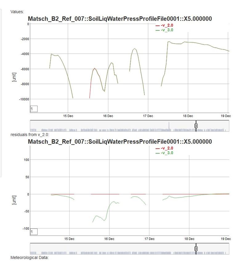
v
List of Figures
1.1 HPC Software Maturity . . . . . . . . . . . . . . . . . . . . . . 2
2.1 Geotop application . . . . . . . . . . . . . . . . . . . . . . . . . 4
2.2 Geotop grid . . . . . . . . . . . . . . . . . . . . . . . . . . . . . 5
2.3 Geotop flowchart . . . . . . . . . . . . . . . . . . . . . . . . . . 8
2.4 Geotop functions . . . . . . . . . . . . . . . . . . . . . . . . . . 10
3.1 Code coverage for 1D tests using gcov. . . . . . . . . . . . . . . 16
4.1 Area surrounding station B2: large view (from Bortoli, 2017) . 22
4.2 Analyzed area for snow test case (from Engel et al., 2017). . . . 23
4.3 View of Montacini study site. . . . . . . . . . . . . . . . . . . . 24
6.1 CPU cycles without execution for the three test cases . . . . . 30
6.2 Cache miss rations for the three test cases . . . . . . . . . . . . 30
6.3 Callgraph for B2 test case using GEOtop 2.0. . . . . . . . . . . 33
6.4 Callgraph for B2 test case using GEOtop 3.0. . . . . . . . . . . 34
6.5 Callgraph for snow test case using GEOtop 2.0. . . . . . . . . . 35
6.6 Callgraph for snow test case using GEOtop 3.0. . . . . . . . . . 36
6.7 Callgraph for Montacini test case using GEOtop 2.0. . . . . . . 37
6.8 Callgraph for Montacini test case using GEOtop 3.0. . . . . . . 38
8.1 Run time for GEOtop 2.0 and default 3.0 . . . . . . . . . . . . . 47
8.2 Run time for GEOtop 2.0 and 3.0 with math optimization . . . 48
8.3 Speed up using OpenMP: whole picture . . . . . . . . . . . . . 50
8.4 Speed up using OpenMP: zoom in . . . . . . . . . . . . . . . . 50
8.5 Speed up of the parallelized functions . . . . . . . . . . . . . . 51
8.6 Speed up of the parallelized functions . . . . . . . . . . . . . . 52
8.7 Run time for GEOtop 2.0 and 3.0 with vectorization . . . . . . 53
8.8 Run time for GEOtop 2.0 and 3.0 in the best case. . . . . . . . . 54
9.1 Examples of different simulated Tsurface between v2.0 and v3.0
for B2 test case. . . . . . . . . . . . . . . . . . . . . . . . . . . . 57
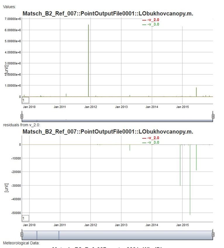
9.2 Example of different simulated LObukhovcanopy between v2.0
and v3.0 for B2 test case. . . . . . . . . . . . . . . . . . . . . . . 59
9.3 Differences in the simulatedSoilLiqWaterPressProfile between v2.0
and v3.0 for B2 test case. . . . . . . . . . . . . . . . . . . . . . . 61
9.4 Example of snowdepth map for snow test case. . . . . . . . . . 62
9.5 Example of snowduration map for snow test case. . . . . . . . 63
9.6 Example of snowmelted map for snow test case. . . . . . . . . 63
9.7 Example of snowduration map for snow test case. . . . . . . . 64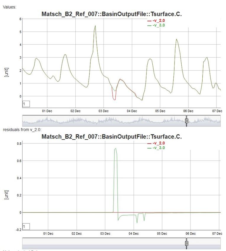
vii

List of Tables

 3.1   Output of Meson test for a 1D short test case. . . . . . . . . . .                       16

 5.1   CPU specifications of my local pc. . . . . . . . . . . . . . . . .                       25
 5.2   CPU specifications of the used node of VSC-3. . . . . . . . . .                          26

 6.1   Cycle activity for B2 test case. . . . . . . . . . . .   .   .   .   .   .   .   .   .   28
 6.2   L2 and L3 cache for B2 test case. . . . . . . . . . .    .   .   .   .   .   .   .   .   29
 6.3   Output of the class Timer for B2 test case. . . . .      .   .   .   .   .   .   .   .   40
 6.4   Output of the class Timer for snow test case. . .        .   .   .   .   .   .   .   .   40
 6.5   Output of the class Timer for Montacini test case.       .   .   .   .   .   .   .   .   41

 9.1   Results of outputs comparison between GEOtop v2.0 and v3.0                               55
 9.2   Tolerance units for each output variable. . . . . . . . . . . . .                        55
 9.3   Output variables (file basin.txt) whose values are different be-
       tween v2.0 and v3.0 for B2 test case. . . . . . . . . . . . . . . .                      56
 9.4   Output variables (file point.txt) whose values are different be-
       tween v2.0 and v3.0 for B2 test case. . . . . . . . . . . . . . . .                      58
 9.5   Statistics of differences, between v2.0 and v3.0, of the pressure
       head at variable depth (file psiz.txt) for B2 test case. . . . . . .                     60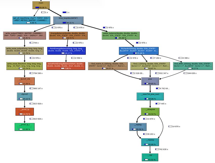
ix
List of Abbreviations
DEM Digital Elevation Model
IHSS Integrated Hydrologic Surface Subsurface
LSM Land Surface Models
LTER Long Term Ecological Research Site
OOP Object Oriented Approach
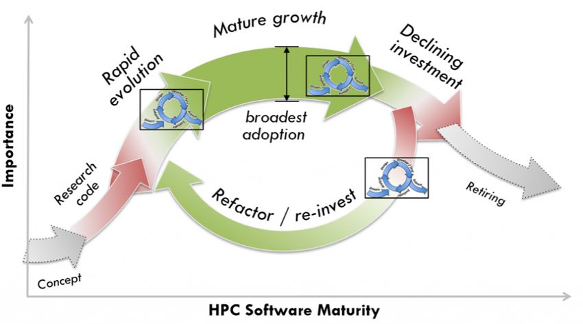
RAII Resource Acquisition Is Initialization1 Chapter 1 Introduction The GEOtop hydrological scientific package is an integrated hydrological model that simulates the heat and water budgets at and below the soil sur- face (Rigon, Bertoldi, and Over, 2006). It describes the three-dimensional water flow in the soil and the energy exchange with the atmosphere, con- sidering the radiative and turbulent fluxes. Furthermore, it reproduces soil freezing and thawing processes, and it simulates the temporal evolution of snow cover, soil temperature and moisture. The model can be applied both at the plot and the catchment scale to study the long term water budget and runoff production. The model has been applied to a variety of scientific prob- lems, ranging from estimation of runoff and water budget in small - medium chatchments (< 1000 m2 ), studies related to the water-soil-vegetation interac- tions, snow cover in mountain areas, climate change impact assessment (for a full reference list see http://geotopmodel.github.io/geotop/materials/ publication-list.html). One version of the model is currently used in an operational snow forecasting system (http://www.mysnowmaps.com). The core components of the package were presented in the 2.0 version (En- drizzi et al., 2014), which was released as Free Software Open-source project under GNU General Public License v3.0. The code was written in C lan- guage. However, despite the high scientific quality of the project, a modern software engineering approach was still missing. Such weakness hindered its computational efficiency, its scientific potential and its use both as a stan- dalone package and, more importantly, in an integrated way with other hy- drological software tools and earth system models. A poor engineering is typical issue of scientific softwares, whose goal is the creation of new scientific knowledge; the emphasis placed on software qual- ity (i.e., correctness of code, maintainability, and reliability) has been his- torically lower than seen in more traditional software engineering (Heaton and Carver, 2015). More in general, the scientific software community is fac- ing a crisis created by the confluence of disruptive changes in computing architectures and new opportunities for greatly improved data availability a simulation capabilities (See the scheme in Fig.1 taken from Ideas Produc- tivity project). There is therefore the need, in order to keep productive well established scientific softwares to perform a software refactoring to develop efficient codes for parallel architecture. A suitable test case is the GEOtop model, an integrated hydrological model which started to be developed in 2000, and, since them, continuously evolved to address a number of scien- tific and applied problems, but also increasing it complexity.
2                                                         Chapter 1. Introduction

          F IGURE 1.1: Schematic representation of the life cycle of a sci-
                entific software (from Ideas Productivity project).

The goal of this project is to perform a software re-engineering and refactor-
ing of the GEOtop model code to create a robust and stable scientific soft-
ware package, optimized for modern parallel clusters, open to the scientific
community, easily usable by researchers and experts, and interoperable with
other packages. Specifically, this thesis aims to:

    • restructure the code from C to C++, taking advantage of an Object-
      Oriented Programming;

    • clean the code, rewriting the old data structures;

    • optimize the maths, replacing the computationally expensive opera-
      tions with faster ones;

    • parallelize the code with OpenMP, to decrease run time.

The thesis is structured as follows. First, will be given a brief overview of the
model structure, code and numeric. Then, the software re-engineering work
will be described in detail. In order to test model performance three repre-
sentative experimental test cases have been selected among the large suite of
possible models configurations. For the selected test cases, a code profiling
has been performed. On the basis of those results a code optimization has
been performed, improving the efficiency of most expensive mathematical
operation and employing OpenMP parallelism for the thread-safe parts of
the code. Then, performances and differences of the re engineered 3.0 code
are compared with the original 2.0 version. Finally, future code develop-
ments towards a further code optimization are discussed.
3
Chapter 2
Model overview
GEOtop simulates the fluxes and budgets of energy and water on a landscape
defined by three-dimensional grid boxes, whose surfaces come from a digi-
tal elevation model (DEM) and whose lower boundaries are located at some
specified spatially varying depth, as shown in Fig. 2.1. Surface boundary
conditions are given by hydrometeorological measurements (rainfall, tem-
perature, wind velocity) (Bertoldi, 2004), regionalized with the approaches
described in Liston and Elder, 2006 or in Bavay and Egger, 2014, depending
on the code version. A general introduction on the model is given in Rigon,
Bertoldi, and Over, 2006. The users manual can be found online here (En-
drizzi et al., 2011). In this thesis only a brief overview will be given.
2.1 Landscape and equation discretization
GEOtop requires preprocessing of the catchment DEM to estimate drainage
directions, slopes, curvature, the channel network structure, shadowing, and
the sky view factor. Surface runoff is modeled to follow the terrain surface
according to a so-called D8 topology as in Orlandini et al., 2003. The DEM
identifies also the plan view of a three-dimensional grid on which all the
model’s equations are discretized. The grid cells are identified as hillslope or
river network cells. River network cells are treated the same as hillslope cells
except for the routing of surface runoff. For each cell, different land cover
and soil properties could be defined.
2.2 Water and energy budgets
The system of equations representing the water balance in the soil is:
ph
∂θw ρ ∂θ
+ i i =0 (2.1)
∂t ρw ∂t
fl
∂θw
+ ∇ · (−K ∇ H ) + Sw = 0 (2.2)
∂t
where dθ ph is the fraction of liquid water content in soil subject to phase
change, dθ f l is the fraction of liquid water content transferred by water flux,4 Chapter 2. Model overview
F IGURE 2.1: Classification of a slope surface in a mountain
basin based on the land cover (from Endrizzi et al., 2011).
ρi is the density of ice, θi is the fraction of ice in soil, K is the hydraulic con-
ductivity, H is the sum of the pressure and potential heads, Sw is the mass
sink term.
The equation representing the energy balance in a soil volume subject to
phase change is:
∂U ph
+ ∇ · G + Sen − ρw [ L f + cw ( T − Tre f )]Sw = 0 (2.3)
∂t
where U ph is the volumetric internal energy of soil subject to phase change,
t is time, ∇· is the divergence operator, G is the heat conduction flux, Sen is
the energy sink term, L f is the latent heat of fusion, ρw is the density of liquid
water in soil, T is the soil temperature and Tre f is the reference temperature
at which the internal energy is calculated.2.3. Numerics 5
F IGURE 2.2: 3D calculation grid and discretization on the x-z
plane; the red points, at the center of the cell, coincide with the
calculation grid points (from Endrizzi et al., 2011).
2.3 Numerics
In this section is reported a synthesis of the GEOtop model numerical ap-
proach, taken from Endrizzi et al., 2017. In order to reduce the complexity of
the numerical method, Eqs. (2.2) and (2.3) are linked in a time-lagged man-
ner, instead of solving them in a fully coupled way. Both equations have the
same form, which can be generalized as:
∂F (κ )
+ ∇ · (−κ (χ)∇χ) + S = 0 (2.4)
∂t
where χ is the unknown function of space and time, F a non-linear function
of the unknown, S is the sink term and κ is a conductivity function of the
unknown.
All the derivates are discretised as finite differences. Therefore the following
relation is obtained.
F (χin+1 ) − F (χin ) M κm
ij
−∑ (χm m
j − χi ) + Si = Gi (2.5)
∆t j
D ij
where the equation is written for the generic i − th cell; n represents the pre-
vious time step (known solution), n + 1 is the next time step (unknown solu-
tion), ∆t is the time step, j is the index of the M adjacent cells with which the
i cell can exchange fluxes, m represents a time instant between n and n + 1,
κij is the conductivity between the cell i and j, Dij is the distance between the
centres of the cells i and j, Si is the sink term and Gi is the residual that is to
be minimized to find a solution.
Eq. (2.5) is a system of N equations and the second term on the left-hand
side is the sum of the fluxes exchanged with the neighbouring cells. The
variables at the instant m are represented with a linear combination between
the instant n and n + 1.6 Chapter 2. Model overview
Several cases are possible:
• m = n: the method is fully explicit and unstable;
• m = n + 1/2: the method has a second order precision but might not
be always stable;
• m = n + 1: the method has a first order precision but is unconditionally
stable.
Since there are more concerns on stability than precision, the last is the chosen
method.
A solution of Eq. (2.5) is sought with a special Newton-Raphson method,
with the following sequence (Kelley, 2003):
χ n +1 = χ n + λ d d ( χ n ) (2.6)
where χ is the vector χi that appears in Eq. (2.5), d denotes the Newton
direction and λd is the path length (a scalar,2.4. Software package 7
2.4 Software package
2.4.1 Simulation flow chart
The model transforms the input given by the user into results, by solving the
energy and mass balance in the calculation domain (Endrizzi et al., 2017). As
reported in Fig. 2.3 GEOtop does the following activities:
• Read input data. In this phase the model reads: (i) the keywords and
parameters specified in the main configuration file called geotop.inpts;
(ii) the topographic maps, as the DEM, the land cover map, and, if avail-
able, the maps with soil type, river drainage networks, the maps with
the initial conditions; (iii) other optional parameters. If a parameter or
a map is not specified with the proper keyword, it assumes a default
value.
• Create and initialize mesh. It creates the calculation mesh according
to the grid size of the land cover map and the vertical nodes spacing
defined for the vertical grid. Then it initializes the temperature and
water pressure head of each node with the initial conditions and sets
the physical parameters according to what specified by the keywords.
• Read meteo data. During this phase, it incorporates the meteorological
input data for each available meteorological station: these data repre-
sent the forcing that will drive the simulation, producing the dynamic
boundary conditions for the surface nodes. Finally, GEOtop sets the ini-
tial simulation time to initialize the simulation counter: this will allow
to compare the current simulation time with the expected simulation
end time
At this point the time loop for the calculation and the printing routines be-
gin. In particular, at each calculation time step, GEOtop fulfills the following
tasks, as illustrated in Fig. 2.3:
• Distribute meteorological forcing. This allows to spatially distribute
the meteorological forcing, measured in discrete meteo station, in all
the calculation cells. This methodology is based on Liston and Elder,
2006, for the code version 2.0, or on the METEO-IO library (Bavay and
Egger, 2014) for the code version 2.1.
• Energy balance. In this phase the energy balance equation is solved.
This encompasses the calculation of the surface energy fluxes, the veg-
etation module, the snow/glacier module and the routine that the cal-
culates the soil temperatures and ice content.
• Water balance. In this phase the mass balance equation is solved. This
encompasses the calculation of the infiltration routine to determine the
pore water pressure and water content through a 3D Richards solver.
Eventually, the runoff and channel routing routines, based on a shallow-
water solver, will allow to determine the discharge at the basin outlet.8 Chapter 2. Model overview
• Write output. This phase is intended to print the point information and
the maps according to the desired output frequency.
• Update and check time. This phase updates the time with the calcu-
lation time step and compares the new time with the simulation end
time, to verify whether to stop the simulation or loop again. The model
uses a dynamic calculation time step. If the convergence criteria is not
reached either for the solution of the energy of the water budget, then
the time step is reduced. If the current simulation time exceeds the end
of the simulation, then the program stops and deallocates all the struc-
tures.
F IGURE 2.3: GEOtop flow chart: model point of view for ac-
complishing a simulation (Courtesy of E. Cordano).
In terms of model functions, the call structure is quite complex. The most
relevant functions calls are illustrated in the scheme of Fig. 2.4, which has
been obtained parsing the source code with Doxygen.2.4. Software package 9
2.4.2 Simulation types
The model can run with two different domain configurations:
• 1D: only vertical fluxes are considered, so mass and energy balance
are performed at local scale. Actually some processes are mainly 1-
dimensional (i.e., soil temperature and snow profiles), therefore they
can be investigated using GEOtop in a simplified manner. In such
a way the computational domain is reduced to one vertical column
aligned to a Cartesian grid. Examples of processes mainly character-
ized by 1D-dynamics are vertical water infiltration, plot scale estima-
tion of snow melt and vegetation processes.
• 3D: both vertical and lateral fluxes are taken into account so balances
are done at basin scale. Examples of processes mainly characterized
by 3D-dynamics are atmosphere-vegetation interactions, groundwater
movement, catchment scale water budgets. Usually this setup needs
more calculations so it is more CPU-intensive.
The model can be also run turning off or on the main processes, which are
the energy budget and the water budget calculation. For example, to sim-
ulate snow dynamics, only the energy budget is needed; to simulate water
infiltration, only the water budget. To simulate in complete way catchment
scale hydrological processes, a 3D calculation of both budgers is needed.
On a typical workstation, a full 3D one year simulation over a grid of about
200x200 pixels could require between 6 and 24 hours of computatio time. For
this reason, there is the need to optmize and parallelize the code in order to
cope with modern scientific and operational needs.10 Chapter 2. Model overview
F IGURE 2.4: Most relevant functions calls of GEOtop derived
from Doxygen. In yellow are underlined the functions linked
with the main physical processes modelled by GEOtop.11
Chapter 3
GEOtop 3.0
3.1 Background
The latest versions of GEOtop are:
• 2.0: written in C, released in 2014 as free software open-source project,
scientifically tested and published. This version is available on the
github repository https://github.com/geotopmodel/geotop at branch
se27xx. However, despite the high scientific quality of the project, a
modern software engineering approach was still missing.
• 2.1: developed from 2014, written in C++, open source and documented
on the same github repository but at branch master. This version, dif-
ferently from the 2.0, was developed from the beggining using the git
version-control system, and Travis-CI (https://docs.travis-ci.com/)
allowed to continuously check the correctness of the build over a wide
number of tests cases.
The main advantage of this new version is the possibility to use Me-
teoIO library (Bavay and Egger, 2014), that provides a uniform inter-
face to meteorological data (https://models.slf.ch/p/meteoio/); un-
fortunately, the output results are different compared to the validated
2.0 and only a few people were working on the scientific validation.
Besides, the code is neither modular nor flexible, and it is characterized
by code repetitions and unsolved bugs, difficult to find.
Hence a new version was needed that had to be scientifically validated, easy
to compile and run, modular and flexible, tested as much as possible and
computationally efficient. The code development will have to fulfill the so
called "best programming practices", a set of rules that have solid founda-
tions in research and experience, and that improve scientists’ productivity
and their software reliability (Wilson et al., 2014). These will be referred and
explained in details in the following sections, when describing the new fea-
tures of GEOtop 3.0; the code package can be found in the same github repos-
itory at branch v3.0.12 Chapter 3. GEOtop 3.0
3.2 Easy to compile and run
Using a build system tool to automate workflows can avoid errors and in-
efficiencies from repeating commands manually (Wilson et al., 2014); this
is one of the "best programming practices", and also a way to simplify the
code compiling, running and debugging. Meson build system tools (https:
//mesonbuild.com/) was used since it is fast, allows for modularity and it can
be easily coupled with gdb (https://www.gnu.org/software/gdb/). How-
ever, the usage of CMake (https://cmake.org/) was preserved to maintain
backward compatibility.
3.3 Modular and flexible
C++ programming language was chosen because, in addition to the facili-
ties provided by C (in which the scientifically validated GEOtop version was
written), it provides flexible and efficient facilities for defining new types
that closely match the concepts of the application: this technique for pro-
gram construction is called data abstraction(Stroustrup, 2013).
These user-defined types are named classes: they are an expanded concept of
data structures, containing a series of variables named members and a series
of procedures named methods. An object of a class contains type information
and it can be used in contexts in which its type cannot be determined at com-
pile time; programs using objects of such types are often called Object-based
or Object-Oriented. The advantages of OOP exploited in GEOtop 3.0 are the
following: (http://www.c4learn.com/cplusplus/oop-advantages/):
(1) it provides a clear modular structure for programs which makes it good
for defining abstract datatypes in which implementation details are
hidden;
(2) objects can also be reused within and across applications, lowering the
cost of development and decreasing potential mistakes;
(3) it makes software easier to maintain and modify, as new objects can be
created with small differences to existing ones;
(4) it has the feature of memory management through RAII (Resource Ac-
quisition Is Initialization) technique, which binds the life cycle of a re-
source (i.e., allocated heap memory) to the lifetime of an object (https:
//en.cppreference.com/w/cpp/language/raii), whose dedicated mem-
ory is allocated by a constructor and deallocated by a destructor, pre-
venting memory leaks.
(5) it is suitable for large projects and fairly efficient.
Moreover, another advantage of C++ is the possibility to write code in a way
that is independent of any particular type thanks to the usage of templates. A
template is a blueprint or formula for creating a generic class or a function,
than can be used with different data types (https://www.tutorialspoint.3.3. Modular and flexible 13
com/cplusplus/cpp_templates.htm): this avoids unnecessary code repeti-
tions and reduce potential mistakes, without penalties at runtime.
Additionally, C++ has a very rich function libraries, designed for portability.
All these new aspects and features, some of which could be considered "best
programming practices" (i.e., (1) makes the code easy to understand and (3)
allows for code reusage) were exploited in the new data structures:
• Vector, Matrix and Tensor (whose some parts are reported
in code boxes 3.4 and 3.5), used to conceptually define vectors, matrices
and tensors;
• RowView and MatrixView, used to respectively access a row
from an object of type Matrix and access a matrix from an object of
type Tensor.
These new classes were defined in a future perspective to allow a rewriting
of the linear algebra and a parallelization, not easily achievable using the
old data structures defined using the fluid turtle library (http://www.ing.
unitn.it/~rigon/FLUIDTURTLE/LIBRARIES/BASICS/).
Now, differently from GEOtop 2.0, the data structures can be accessed in a
uniform way by the user thanks to the operator overloading, and, in order to
prevent mistakes, only the interfaces are exposed, while the implementation
details (i.e., private class members) are hidden from outside of the class, ac-
cording to data-hiding technique (1).
Moreover in the new data structures some "special" operators were defined
not only to simply access an element of the structure (i.e., []) but also to per-
form a bound check (i.e. ()) as it will be explained in section 3.4.
Actually, in GEOtop 2.0, the element indexing was not equal for all the vari-
ables, whose first index could be 0 (like C/C++) or 1 (like Fortran); the latter
was the default choice (code boxes 3.2 and 3.3) so in the former case another
allocation function was used (code box 3.1). This error-prone technique led to
segmentation fault for some tests; the issues were solved, during the debug
phase, thanks exactly to the development of the () operator.
DOUBLEVECTOR ∗ new_doublevector0 ( long nh )
{
DOUBLEVECTOR ∗m;
m=(DOUBLEVECTOR ∗ ) malloc ( s i z e o f (DOUBLEVECTOR) ) ;
i f ( !m) t _ e r r o r ( " a l l o c a t i o n f a i l u r e i n DOUBLEVECTOR( ) " ) ;
m−>isdynamic=isDynamic ;
m−>n l = 0 ;
m−>nh=nh ;
m−>co= d v e c t o r (m−>nl , nh ) ;
r e t u r n m;
}
L ISTING 3.1: Vector allocation for GEOtop 2.0 using the first
index equal to 0 (alloc.c)14 Chapter 3. GEOtop 3.0
# d e f i n e NL 1 /∗ Numerical R e c i p e s a l l o c a t i o n r o u t i n e s allow t o have
a r b i t r a r y s u b s c r i p t s f o r v e c t o r and m a t r i x e s .
The f l u i d t u r t l e l i b r a r y r e s t r i c t t h i s freedom by
setting
t h e i r lower value t o NL ∗/
L ISTING 3.2: Definition of the lower bound for a data structure
in GEOtop 3.0 (turtle.h)
DOUBLEVECTOR ∗ new_doublevector ( long nh )
{
DOUBLEVECTOR ∗m;
m=(DOUBLEVECTOR ∗ ) malloc ( s i z e o f (DOUBLEVECTOR) ) ;
i f ( !m) t _ e r r o r ( " a l l o c a t i o n f a i l u r e i n DOUBLEVECTOR( ) " ) ;
m−>isdynamic=isDynamic ;
m−>n l =NL;
m−>nh=nh ;
m−>co= d v e c t o r (m−>nl , nh ) ;
r e t u r n m;
}
L ISTING 3.3: Vector allocation for GEOtop 2.0 using the first
index equal to 1 (alloc.c)
# i n c l u d e " matrix . h "
# i n c l u d e " matrixview . h "
t e m p l a t e < c l a s s T> c l a s s RowView ;
t e m p l a t e < c l a s s T> c l a s s MatrixView ;
t e m p l a t e < c l a s s T> c l a s s Tensor {
public :
...
/∗∗ Given a l a y e r ( k ) and a row ( i ) , i t g i v e s a l l t h e elements
∗∗ c o r r i s p o n d i n g t o d i f f e r e n t columns ∗/
RowView row ( c o n s t s t d : : s i z e _ t k , c o n s t s t d : : s i z e _ t i ) {
GEO_ASSERT_IN_RANGE( k , ndl , ndh ) ;
GEO_ASSERT_IN_RANGE( i , n r l , nrh ) ;
r e t u r n RowView { &co [ ( i −n r l ) ∗ n _ c o l + ( k−ndl ) ∗ ( n_row∗
n _ c o l ) ] , nch , n c l } ;
};
MatrixView matrix ( c o n s t s t d : : s i z e _ t k ) {
GEO_ASSERT_IN_RANGE( k , ndl , ndh ) ;
r e t u r n MatrixView { &co [ ( k−ndl ) ∗ ( n_row∗ n _ c o l ) ] , nrh , n r l
, nch , n c l } ;
};
L ISTING 3.4: Part of the header file tensor.h of GEOtop 3.0
showing modularity (1) and code reusage (2)3.4. Tested as much as possible 15
∗ constructor
∗ @param _ n r l , _nrh lower and upper bound f o r rows
∗ @param _ncl , _nch lower and upper bound f o r columns
∗ @param _ndl , _ndh lower and upper bound f o r depth
∗/
Tensor ( c o n s t s t d : : s i z e _ t _ndh , c o n s t s t d : : s i z e _ t _ndl ,
c o n s t s t d : : s i z e _ t _nrh , c o n s t s t d : : s i z e _ t _ n r l ,
c o n s t s t d : : s i z e _ t _nch , c o n s t s t d : : s i z e _ t _ n c l ) :
ndh { _ndh } , ndl { _ndl } , nrh { _nrh } , n r l { _ n r l } , nch { _nch } , n c l { _ n c l
},
n_dep { ndh−ndl + 1 } , n_row { nrh−n r l + 1 } , n _ c o l { nch−n c l + 1 } ,
co { new T [ ( ndh−ndl +1) ∗ ( nrh−n r l +1) ∗ ( nch−n c l +1) ] { } } { } // i n i t
to 0
Tensor ( c o n s t s t d : : s i z e _ t d , c o n s t s t d : : s i z e _ t r , c o n s t s t d : :
size_t c ) :
Tensor { d , 1 , r , 1 , c , 1 } { }
/∗∗ d e s t r u c t o r . d e f a u l t i s f i n e ∗/
~Tensor ( ) = d e f a u l t ;
L ISTING 3.5: Part of the header file tensor.h. of GEOtop 3.0
showing the application of RAII concept (4)
3.4 Tested as much as possible
Coverage analysis of a program can be a significant component in confident
assessment of overall software quality since it gives a clear measure of code
testing (Horgan, London, and Lyu, 1994), allowing to discover its untested
parts.
Gcov coverage testing tool (https://gcc.gnu.org/onlinedocs/gcc/Gcov.html)
together with Lcov graphical front-end, were used to find what lines of code
were actually executed. Actually Lcov collects gcov data for multiple source
files and creates HTML pages containing the source code annotated with cov-
erage information, also adding overview pages for easy navigation within
the file structure (http://ltp.sourceforge.net/coverage/lcov.php).
Analyzing the code coverage for all the 1D tests (Fig. 3.1) it was noticed that
many lines and functions were not used; for example in the source file blow-
ingsnow.cc, dealing with snow transport and deposition, < 30% of functions
were used: this could happen because it was not snowing or because some
functions should have been used but they were not.16 Chapter 3. GEOtop 3.0
F IGURE 3.1: Code coverage for 1D tests using gcov.
In order to improve code reliability, a testing suite was set, comprising:
(1) 1D and 3D short test cases, consisting in the check of effective run of the
executable with the all the inputs of 1D and 3D cases provided in the git
repository, plus a comparison of output results between the 3.0 and 2.0
version, making the test passing if the absolute and relative differences
were < 10−5 ;
(2) unit tests for all the new added code (i.e. constructors, initialization and
functions of the new data structures) using the Google test framework
(https://github.com/google/googletest);
(3) bound checking when accessing elements of the new data structures;
this is possible thanks to the access operator () that performs a range
check when the code is compiled in debug mode.
For istance, to run all the 1D and 3D short test cases (1) the command that
has to be typed in the build folder is:
meson test --suite geotop:1D --suite geotop:3D
and the output for every test will show the test name (i.e., Bro) and the sim-
ulation type (i.e., 1D) (see Tab. 3.1).
TABLE 3.1: Output of Meson test for a 1D short test case.
1/2 geotop:1D+Bro / 1D/Bro OK 11.13 s
2/2 geotop:1D+Bro / 1D/Bro.test_runner OK 3.48 s3.4. Tested as much as possible 17
Examples of unit tests (2) are provided in the code boxes 3.6 and 3.7 where
the correctness check is done in the expression EXPECT_EQ, performing a com-
parison between the first value, provided by the developer (since he/she al-
ready knows it for a simple case) and the second, calculated using the newly
written code; if the two values are different, a statement error will be printed
with both, allowing the developer to understand what happened.
TEST ( Matrix , c o n s t r u c t o r _ 2 a r g s ) {
Matrix < i n t > m{ 3 , 5 } ; // 3 x5 matrix
EXPECT_EQ ( s t d : : s i z e _ t { 3 } , m. n_row ) ;
EXPECT_EQ ( s t d : : s i z e _ t { 5 } , m. n _ c o l ) ;
}
L ISTING 3.6: Unit tests for the constructor of a Matrix.
TEST ( Matrix , i n i t i a l i z a t i o n ) {
Matrix < i n t > m{ 2 , 2 } ; // 2 x2 matrix
EXPECT_EQ ( 0 , m( 1 , 1 ) ) ;
EXPECT_EQ ( 0 , m( 1 , 2 ) ) ;
EXPECT_EQ ( 0 , m( 2 , 1 ) ) ;
EXPECT_EQ ( 0 , m( 2 , 2 ) ) ;
# i f n d e f NDEBUG
EXPECT_ANY_THROW( m( 0 , 0 ) ) ;
EXPECT_ANY_THROW( m( 3 , 3 ) ) ;
# else
EXPECT_NO_THROW( m( 0 , 0 ) ) ;
EXPECT_NO_THROW( m( 3 , 3 ) ) ;
# endif
}
L ISTING 3.7: Unit tests for the initialization of a Matrix.
Examples of the access operator (3) for the class Vector was developed as
shown in the code box 3.8 and 3.9; it can be noticed that the operator (), when
the compiling mode is:
• RELEASE: it returns just the element, recalling the operator [];
• DEBUG: it calls the range-checked access operator at, which uses the
macro GEO_ERROR_IN_RANGE, checking that the accessed index (i) is be-
twen the lower (nl) and upper (nh) bound of the vector.
/∗∗ range −checked a c c e s s o p e r a t o r ∗/
T &a t ( c o n s t s t d : : s i z e _ t i ) {
GEO_ERROR_IN_RANGE( i , nl , nh ) ;
return (∗ t h i s ) [ i ] ;
}
L ISTING 3.8: Definition of the range-checked access operator
for Vector.18 Chapter 3. GEOtop 3.0
T &o p e r a t o r ( ) ( c o n s t s t d : : s i z e _ t i )
# i f d e f NDEBUG
noexcept
# endif
{
# i f n d e f NDEBUG
return at ( i ) ;
# else
return (∗ t h i s ) [ i ] ;
# endif
}
L ISTING 3.9: Definition of the access operator for Vector.
3.5 Computationally efficient
Several optimizations were implemented: all of them can be activated by
a flag (as explained in Chapter 8) except one, that is the inline of all the
functions in the previous existing source files pedo.func.cc, containing pedo-
transfer functions and statistic functions, and util_math.cc, containing math-
ematical rules to solve a linear system.
Inline function is an optimization technique used by the compilers espe-
cially to reduce the execution time (http://www.cplusplus.com/articles/
2LywvCM9/). When the compiler inline-expands a function call, the func-
tion’s code gets inserted into the caller’s code stream: this can improve per-
formance, because the optimizer can procedurally integrate the called code
(https://isocpp.org/wiki/faq/inline-functions).
Since the functions in pedo.func.cc and util_math.cc are very much used and
are called thousands of time during a test run (see Chapter 7), they were put
in the correspondent header files pedo.func.h and util_math.h preceded by
the keywords inline. Examples of inlined functions are reported in the code
boxes 3.10 and 3.11.
i n l i n e double t h e t a _ f r o m _ p s i ( double psi , double i c e , long l ,
MatrixView &&pa , double pmin )
{
const double s = pa ( j s a t , l ) ;
const double r e s = pa ( j r e s , l ) ;
const double a = pa ( j a , l ) ;
const double n = pa ( j n s , l ) ;
const double m = 1. − 1./n ;
const double Ss = pa ( j s s , l ) ;
r e t u r n t e t a _ p s i ( psi , i c e , s , r e s , a , n , m, pmin , Ss ) ;
}
L ISTING 3.10: Function inline of theta_from_psi in pedo.func.h.3.5. Computationally efficient 19
i n l i n e double adaptiveSimpsons2 ( double ( ∗ f ) ( double x , void ∗p ) ,
void ∗ arg , // p t r t o f u n c t i o n
double a , double b , // i n t e r v a l [ a , b ]
double e p s i l o n , // e r r o r t o l e r a n c e
i n t maxRecursionDepth ) // r e c u r s i o n
cap
{
double c = ( a + b ) /2 , h = b − a ;
double f a = f ( a , arg ) , f b = f ( b , arg ) , f c = f ( c , arg ) ;
double S = ( h/6) ∗ ( f a + 4∗ f c + f b ) ;
r e t u r n adaptiveSimpsonsAux2 ( f , arg , a , b , e p s i l o n , S , fa , fb ,
fc ,
maxRecursionDepth ) ;
}
L ISTING 3.11: Function inline of adaptiveSimpsons2 in
util_math.h.21 Chapter 4 Test cases One of the major challenges in testing the GEOtop model code is related to the fact that this kind of integrated models can be used in a very wide range of operational conditions and spatial scales. Very different environments and climatic conditions can be considered. Addressed scientific topics range from the classical hydrologicals ones (i.e. runoff prediction) to ecological ones (i.e Evapotranspiration estimation), mountain cryospehere (i.e. snow processes). Typical model’s applications are climate change impacts or risks assessments, as floods or droughts or landslides instability problems. This implies that it is quite challenging to test all the parts of the code. Moreover, the performances and the relative use of the different parts of code depend on the specific pro- cess considered. In the GEOtop v.3 version a suite of more than 10 1D and 20 3D test cases are considered (https://github.com/geotopmodel/geotop/tree/v3.0/tests/), to cover the wide range of scientific problems than can be addressed by the GEOtop model. However, for in this thesis three test cases are analyzed: one 1D case, Matsch_B2_Ref_007, representative of a full calculation of the water and energy budget at local scale, and two 3D cases, snow_dstr_SENSITIVITY, with only the energy budget and snow processes in winter and Muntats- chini_ref_005, with both water and energy budget in summer. The three test cases were run for both a short and long time period for a detailed profiling and to check the optimization improvements on both short and long runs.
22 Chapter 4. Test cases
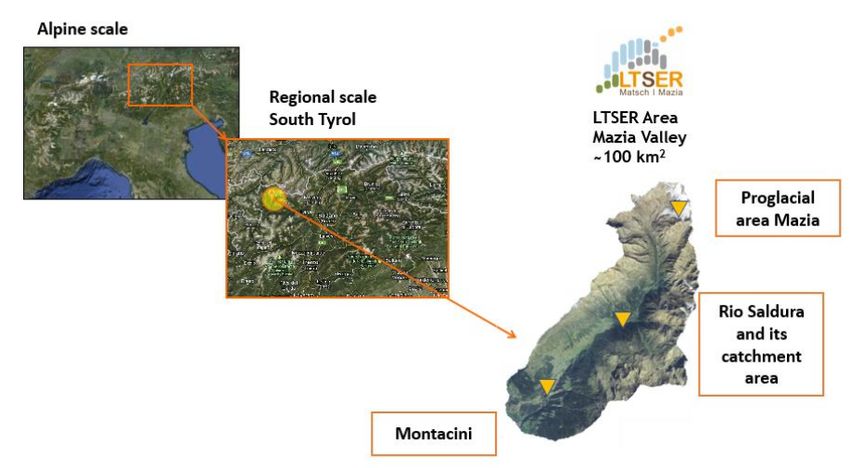
4.1 Matsch_B2_Ref_007
The test involves a hydro-meteorological stations named B2 and located in
Montacini, a Long Term Ecological Research site (LTER) of the Mazia Valley
(South Tyrol, Italy). The station is located at 1480 m a.s.l. in a mountain
meadow area and it is characterized by a sandy loam soil (Bortoli, 2017). The
GEOtop model has been already applied and scientifically validated against
field observations in the work of Della Chiesa et al., 2014 and of Bortoli, 2017.
The model has been employed in 1D mode activating the simulation of both
water and energy budgets. The simulated time is:
• 1 month for the short test (02/10/2009 00:00 - 02/11/2009 00:00);
• ~5 years for the long test (02/10/2009 00:00 - 31/12/2015 23:00).
F IGURE 4.1: Area surrounding station B2: large view (from Bor-
toli, 2017)
.4.2. snow_dstr_SENSITIVITY 23
4.2 snow_dstr_SENSITIVITY
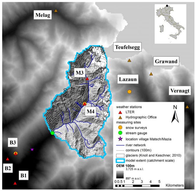
The test is about the simulation of snow processes in the upper Saldura
catchment, a small high-elevation catchment which is also part of the LTER
Mazia, located in the upper Venosta valley (South Tyrol, Italy) (Engel et al.,
2017). The input meteorological stations, indicated in Fig.4.2, are seven: B1,
B2, B3, M3, M4, belonging to EURAC in the framework of the LTER, and
Teufelsegg and Grawand, operated by the Hydrographic Office of the Au-
tonomous Province of Bolzano. The GEOtop model has been scientifically
validated against field observations in the work of Engel et al., 2017.
The model has been employed in 3D mode activating the simulation of only
the energy budget.
The study area is 61 km2 and the set cells are 10’140. The simulated time is:
• 1 day for the short test (26/03/2010 17:00 - 27/03/2010 17:00);
• 1 month for the long test (26/03/2010 17:00 - 26/04/2010 17:00).
F IGURE 4.2: Analyzed area for snow test case (from Engel et al.,
2017).24 Chapter 4. Test cases
4.3 Muntatschini_ref_005
The study area in this test is Montacini (Figure 4.3): it is characterized by ele-
vations between 900 and 2200 m a.s.l. and the main land covers are meadows
and pastures. The input meteorological stations are four: B1, B2, B3, P2, all
of them are LTER sites. The GEOtop model has been already applied and
scientifically validated against field observations in the work of Della Chiesa
et al., 2014 and of Bortoli, 2017.
The study area is ~4 km2 and the set cells are 15’600. The simulated time is:
• 1 day for the short test (26/03/2010 17:00 - 03/10/2009 00:00);
• 1 week for the long test (02/10/2009 00:00 - 09/10/2009 00:00).
F IGURE 4.3: View of Montacini study site.25
Chapter 5
Used architectures
5.1 Local pc
My local pc was used for profiling and for checking eventual improvements
of the optimization. The CPU and cache characteristics are reported in Tab.
5.1; the total RAM is 16 GB. From now it will be referred with the name of
CPU line Intel Core.
TABLE 5.1: CPU specifications of my local pc.
Architecture: x86_64
CPU op-mode(s): 32-bit, 64-bit
Byte Order: Little Endian
CPU(s): 8
On-line CPU(s) list: 0-7
Thread(s) per core: 2
Core(s) per socket: 4
Socket(s): 1
NUMA node(s): 1
Vendor ID: GenuineIntel
CPU family: 6
Model: 94
Model name: Intel(R) Core(TM) i7-6700HQ CPU @ 2.60GHz
Stepping: 3
CPU MHz: 800.007
CPU max MHz: 3500,0000
CPU min MHz: 800,0000
BogoMIPS: 5183.87
Virtualization: VT-x
L1d cache: 32K
L1i cache: 32K
L2 cache: 256K
L3 cache: 6144K
NUMA node0 CPU(s): 0-726 Chapter 5. Used architectures
5.2 VSC-3
The VSC-3 is an HPC system that was installed in summer 2014 at the Arsenal
TU building (Objekt 214) in Vienna by Opens external link in new window-
ClusterVision (http://vsc.ac.at/systems/vsc-3/).
It consists of 2020 nodes, each equipped with 2 processors belonging to the
Ivy Bridge-EP family and internally connected with an Intel QDR-80 dual-
link high-speed InfiniBand fabric.
VSC-3 was used to measure optimization improvements for long tests.
Compiling and running were done specifically on two nodes: n22-029 and
n23-030, having the same specifics reported in Tab. 5.2; the total RAM is 128
GB. From now it will be referred with the name of CPU line Intel Xeon.
TABLE 5.2: CPU specifications of the used node of VSC-3.
Architecture: x86_64
CPU op-mode(s): 32-bit, 64-bit
Byte Order: Little Endian
CPU(s): 32
On-line CPU(s) list: 0-31
Thread(s) per core: 2
Core(s) per socket: 8
Socket(s): 2
NUMA node(s): 2
Vendor ID: GenuineIntel
CPU family: 6
Model: 62
Model name: Intel(R) Xeon(R) CPU E5-2650 v2 @ 2.60GHz
Stepping: 4
CPU MHz: 1199.960
CPU max MHz: 3400,0000
CPU min MHz: 1200,0000
BogoMIPS: 5200.24
Virtualization: VT-x
L1d cache: 32K
L1i cache: 32K
L2 cache: 256K
L3 cache: 20480K
NUMA node0 CPU(s): 0-7,16-23
NUMA node1 CPU(s): 8-15,24-3127
Chapter 6
Profiling
In order to find and track performance bottlenecks, the code was profiled
with:
(1) likwid-perctr, that counts hardware performance events (https://github.
com/RRZE-HPC/likwid/wiki/likwid-perfctr)
(2) callgrind, that records the call history among functions in the program’s
run as a call-graph (http://valgrind.org/docs/manual/cl-manual.
html); this was used together with KCachegrind, a profile data visu-
alization (https://kcachegrind.github.io/html/Home.html).
Moreover, a class Timer(3) was implemeted with which it was possible to
measure the number of calls and time of some specific functions.
The profiling using (1) and (2) was done for both GEOtop versions 2.0 and
3.0 but considering only short tests due to the profiling overhead.
The analysis using (3) were performed only for GEOtop 3.0, since it involves
the addition of some lines of C++ code, but both short and long tests were
done.
All the profiling tests were performed only on Intel Core.
6.1 Likwid-perfctr
The analyzed groups during the runs for the short tests were:
• CYCLE_ACTIVITY, that measures cycle activities, giving an idea of the
stalls caused by data traffic in the cache hierarchy;
• L2CACHE, that measures L2 cache miss rate/ratio, telling how many of
the memory references required a cache line to be loaded from a higher
level;
• L3CACHE, that measures L3 cache miss/ratio.
The typed commands was:
likwid-perfctr -g CYCLE_ACTIVITY -C 0 -g L2CACHE -g L3CACHE ./geotop TEST_DIR
The output of the first run for B2 test case and GEOtop 3.0 is reported in Tabs.
6.1 and 6.2.28 Chapter 6. Profiling
TABLE 6.1: Cycle activity for B2 test case.
Group 1: CYCLE_ACTIVITY
+-----------------------------------+---------+-------------+
| Event | Counter | Core 0 |
+-----------------------------------+---------+-------------+
| INSTR_RETIRED_ANY | FIXC0 | 13075903238 |
| CPU_CLK_UNHALTED_CORE | FIXC1 | 6804707416 |
| CPU_CLK_UNHALTED_REF | FIXC2 | 5092016616 |
| CYCLE_ACTIVITY_STALLS_L2_PENDING | PMC0 | 24212141 |
| CYCLE_ACTIVITY_STALLS_LDM_PENDING | PMC1 | 170785944 |
| CYCLE_ACTIVITY_STALLS_L1D_PENDING | PMC2 | 29946993 |
| CYCLE_ACTIVITY_CYCLES_NO_EXECUTE | PMC3 | 876910168 |
+-----------------------------------+---------+-------------+
+--------------------------------------------+-----------+
| Metric | Core 0 |
+--------------------------------------------+-----------+
| Runtime (RDTSC) [s] | 2.0007 |
| Runtime unhalted [s] | 2.6253 |
| Clock [MHz] | 3463.7965 |
| CPI | 0.5204 |
| Cycles without execution [%] | 12.8868 |
| Cycles without execution due to L1D [%] | 0.4401 |
| Cycles without execution due to L2 [%] | 0.3558 |
| Cycles without execution due to memory [%] | 2.5098 |
+--------------------------------------------+-----------+6.1. Likwid-perfctr 29
TABLE 6.2: L2 and L3 cache for B2 test case.
Group 2: L2CACHE
+-----------------------+---------+-------------+
| Event | Counter | Core 0 |
+-----------------------+---------+-------------+
| INSTR_RETIRED_ANY | FIXC0 | 15334903216 |
| CPU_CLK_UNHALTED_CORE | FIXC1 | 6726320670 |
| CPU_CLK_UNHALTED_REF | FIXC2 | 5004954900 |
| L2_TRANS_ALL_REQUESTS | PMC0 | 1100691015 |
| L2_RQSTS_MISS | PMC1 | 217028917 |
+-----------------------+---------+-------------+
+----------------------+-----------+
| Metric | Core 0 |
+----------------------+-----------+
| Runtime (RDTSC) [s] | 2.0001 |
| Runtime unhalted [s] | 2.5950 |
| Clock [MHz] | 3483.4544 |
| CPI | 0.4386 |
| L2 request rate | 0.0718 |
| L2 miss rate | 0.0142 |
| L2 miss ratio | 0.1972 |
+----------------------+-----------+
Group 3: L3CACHE
+--------------------------+---------+------------+
| Event | Counter | Core 0 |
+--------------------------+---------+------------+
| INSTR_RETIRED_ANY | FIXC0 | 3703676320 |
| CPU_CLK_UNHALTED_CORE | FIXC1 | 1405487046 |
| CPU_CLK_UNHALTED_REF | FIXC2 | 1046429388 |
| MEM_LOAD_RETIRED_L3_HIT | PMC0 | 534619 |
| MEM_LOAD_RETIRED_L3_MISS | PMC1 | 3678 |
| UOPS_RETIRED_ALL | PMC2 | 4183712511 |
+--------------------------+---------+------------+
+----------------------+--------------+
| Metric | Core 0 |
+----------------------+--------------+
| Runtime (RDTSC) [s] | 0.4295 |
| Runtime unhalted [s] | 0.5422 |
| Clock [MHz] | 3481.3657 |
| CPI | 0.3795 |
| L3 request rate | 0.0001 |
| L3 miss rate | 8.791235e-07 |
| L3 miss ratio | 0.0068 |
+----------------------+--------------+30 Chapter 6. Profiling
The previous command was run three times to consider some statistics
and the average among the measurements were analyzed; the focus was on
CPU cycles without execution in total and only due to memory (Fig. 6.1) and
L2 and L3 cache misses (Fig. 6.2). Comparing GEOtop 2.0 and 3.0:
• CPU cycles without execution: decrease for all the test cases, more
markedly for Montacini;
• CPU cycles without execution due to memory: decrease for B2 and
Montacini but slightly increase for snow: anyway for the latter the in-
crease is of the same order of the measurement variations;
• L2 cache misses: decrease for snow and Montacini but increase for B2,
slightly but not within measurement tolerance;
• L3 cache misses: decrease for B2 but increase for snow and Montacini,
again more than the measurement variations.
F IGURE 6.1: CPU cycles without execution, total and only due
to memory, of the two GEOtop versions for the three test cases.
F IGURE 6.2: L2 and L3 cache miss ratios for the two GEOtop
versions of the three test cases.6.2. Callgrind 31
6.2 Callgrind
The command used to produce the output file needed to callgrind was:
valgrind --tool=callgrind --dump-instr=yes ./geotop TEST_DIR
where
• -dump-instr=yes specifies that event counting should be performed at
per-instruction granularity and allows for assembly code annotation
• TEST_DIR is the directory of the selected short test.
The command to read the file using Qcachegrind, included in KCachegrind
package, was:
./qcachegrind callgrind.out.0123
The call graph for the two GEOtop versions for a specific test case displayed
the same structure and more or less the same CPU cycles values, indicated
for every function inside the rectangular boxes, and the same number of calls,
showed over the box.
Analyzing B2 it can be noticed that for both 2.0 and 3.0 (Fig. 6.3 and 6.4):
• most of the CPU cycles is spent doing calculations (time_loop) and only
a few percent in reading the input (get_all_input)
• the water budget calculation dominates (water_balance, and precisely
Richards1D since B2 has a 1D setup) but I/O is important (write_output)
• pow() function is too expensive (50%)
Analyzing snow it can be noticed that, for GEOtop 2.0 (Fig. 6.5):
• most of the CPU cycles is now spent in reading the input (get_all_input),
and especially in computing the sky view factor from the given data;
• energy budget (EnergyBalance) plays anyway an important role (also
because water balance is not considered as explained in Chapter 4);
• the function AdaptiveSimpsonAux2 is called millions of time;
• pow() is present (20%).
Instead, for GEOtop 3.0, in which some functions were inlined (see Section
3.5) it can be noticed (Fig. 6.6):
• most of CPU cycle is spent in reading the input;
• all the functions involved in the energy balance and previously written
inside util_math.cc were not shown by the profiler, indicating that they
involved a low percentage of CPU cycles.32 Chapter 6. Profiling
Analyzing Montacini it can be noticed that, for GEOtop 2.0 (Fig. 6.7):
• water budget dominates (water_balance, and precisely Richards3D since
Montacini has a 3D setup);
• pow() is even more expensive than B2 (70%);
Instead, for GEOtop 3.0 (inline of some functions) it can be noticed (Fig. 6.8):
• water budget dominates but copy_snowvar3D appears in the callgraph;
• pow() is still significant in terms of CPU cycle percentage.6.2. Callgrind 33
F IGURE 6.3: Callgraph for B2 test case using GEOtop 2.0.34 Chapter 6. Profiling
F IGURE 6.4: Callgraph for B2 test case using GEOtop 3.0.6.2. Callgrind 35
F IGURE 6.5: Callgraph for snow test case using GEOtop 2.0.36 Chapter 6. Profiling
F IGURE 6.6: Callgraph for snow test case using GEOtop 3.0.6.2. Callgrind 37
F IGURE 6.7: Callgraph for Montacini test case using GEOtop
2.0.38 Chapter 6. Profiling
F IGURE 6.8: Callgraph for Montacini test case using GEOtop
3.0.6.3. Class Timer 39
6.3 Class Timer
A new class Timer was written to measure the number of calls and CPU time,
both in absolute values and in percentage compared to the total run, of some
relevant functions pointed out by the profiling (and/or already known by
GEOtop users and developers to be expensive). In this section the three short
test cases were analyzed.
c l a s s Timer {
void print_summary ( ) ;
high_resolution_clock : : time_point t _ s t a r t ;
s t d : : map< s t d : : s t r i n g , ClockMeasurements > t im es ;
public :
Timer ( ) : t _ s t a r t { h i g h _ r e s o l u t i o n _ c l o c k : : now ( ) } { }
~Timer ( ) {
# i f n d e f MUTE_GEOTIMER
print_summary ( ) ;
# endif
}
c l a s s ScopedTimer ;
};
L ISTING 6.1: Class Timer measuring function calls and CPU
times.
For B2 can be noticed that:
• the results obtained by callgrind regarind water_balance and I/O are
confirmed;
• atm_transmittance is the most called function, justifying its inline;
• about 18% of the time is used by input file readings and data structure
filling, an action which is done only at the beginning of the simulation;
• about 25% of the time is used by output file readings and data structure
filling, an action done at the output time step, which is usually longer
than the internal calculation time step;
• about 54% of the time is taken by the two main computational tasks
water and energy balance. Those functions are called every computa-
tion time steps. This means that, the longer is the simulation period,
the bigger is the cumulative time required by those functions.
For snow it can be noticed that:
• even if Callgrind indicated that most of the CPU cycles were spent in
reading the input, the most expensive part on a time basis is the energy
balance, summing up to the 57% of the simulation time;
• atm_transmittance is again the most called function, and this time it has
more influence in the total CPU time than for B2;
• sky_view_factor is quite time-expensive, even if not as much as in terms
of CPU cycles. However, this function is called only once at the begin-
ning of the simulation.40 Chapter 6. Profiling
TABLE 6.3: Output of the class Timer for B2 test case.
+---------------------------------------------+------------+------------+
| Total CPU time elapsed since start | 1.98s | |
| | | |
| Section | no. calls | CPU time | % of total |
+---------------------------------+-----------+------------+------------+
| atm_transmittance | 44730 | 0.04s | 1.9% |
| copy_snowvar3D | 5952 | 0.02s | 1.0% |
| SolvePointEnergyBalance | 2994 | 0.19s | 9.6% |
| Richards1D | 2976 | 0.68s | 34.4% |
| water_balance | 2976 | 0.68s | 34.6% |
| write_output | 2976 | 0.49s | 24.7% |
| EnergyBalance | 2976 | 0.39s | 19.6% |
| PointEnergyBalance | 2976 | 0.37s | 18.4% |
| find_matrix_K_1D | 2976 | 0.30s | 15.2% |
| write_snow_file | 2980 | 0.29s | 14.9% |
| get_all_input | 1 | 0.37s | 18.5% |
+---------------------------------+-----------+------------+------------+
Actually CPU cycles can have difference time duration, so there is no guar-
antee that the relative importance of a function in terms of CPU cycles is the
same of its relevance on CPU times basis.
TABLE 6.4: Output of the class Timer for snow test case.
+---------------------------------------------+------------+------------+
| Total CPU time elapsed since start | 9.04s | |
| | | |
| Section | no. calls | CPU time | % of total |
+---------------------------------+-----------+------------+------------+
| atm_transmittance | 3102463 | 2.90s | 32.1% |
| PointEnergyBalance | 6781 | 5.18s | 57.3% |
| SolvePointEnergyBalance | 6781 | 0.54s | 6.0% |
| write_snow_file | 24 | 0.00s | 0.00% |
| copy_snowvar3D | 4 | 0.03s | 0.3% |
| EnergyBalance | 1 | 5.18s | 57.3% |
| get_all_input | 1 | 3.77s | 41.7% |
| sky_view_factor | 1 | 3.35s | 37.1% |
| write_output | 1 | 0.01s | 0.00% |
+---------------------------------+-----------+------------+------------+6.3. Class Timer 41
For Montacini it can be noticed that:
• water_balance is the most time-consuming function, having higher rel-
evance in terms of CPU-time than CPU-cycles;
• copy_snowvar3D appears but with less importance in time than cycles;
• atm_transmittance is again the most called function but it does not af-
fect too much the total CPU time.
• Input/Output functions require a relatively small amount of time.
TABLE 6.5: Output of the class Timer for Montacini test case.
+---------------------------------------------+------------+------------+
| Total CPU time elapsed since start | 86.5s | |
| | | |
| Section | no. calls | CPU time | % of total |
+---------------------------------+-----------+------------+------------+
| atm_transmittance | 3135930 | 2.32s | 2.7% |
| PointEnergyBalance | 143064 | 21.00s | 24.3% |
| SolvePointEnergyBalance | 143064 | 10.16s | 11.7% |
| find_f_3D | 52 | 13.96s | 16.2% |
| copy_snowvar3D | 48 | 0.99s | 1.1% |
| Richards3D | 24 | 63.18s | 73.1% |
| water_balance | 24 | 63.24s | 73.1% |
| find_matrix_K_3D | 24 | 40.98s | 47.4% |
| EnergyBalance | 24 | 21.17s | 24.5% |
| write_output | 24 | 0.51s | 0.6% |
| get_all_input | 1 | 0.45s | 0.5% |
+---------------------------------+-----------+------------+------------+
The output measurements for long tests are instead discussed in Chapter 8,
since it will be used to compare GEOtop 3.0 with and without optimizations,
activated by flags.
The measurements are active by default; if someone is not interested in,
he/she has to type in the build directory
meson configure -DMUTE_GEOTIMER=true
and nothing regarding time will be printed.You can also read