Supplement of Weakened impact of the Atlantic Niño on the future equatorial Atlantic and Guinea Coast rainfall
←
→
Page content transcription
If your browser does not render page correctly, please read the page content below
Supplement of Earth Syst. Dynam., 13, 231–249, 2022
https://doi.org/10.5194/esd-13-231-2022-supplement
© Author(s) 2022. CC BY 4.0 License.

Supplement of
Weakened impact of the Atlantic Niño on the future
equatorial Atlantic and Guinea Coast rainfall
Koffi Worou et al.

Correspondence to: Koffi Worou (koffi.worou@uclouvain.be)

The copyright of individual parts of the supplement might differ from the article licence.
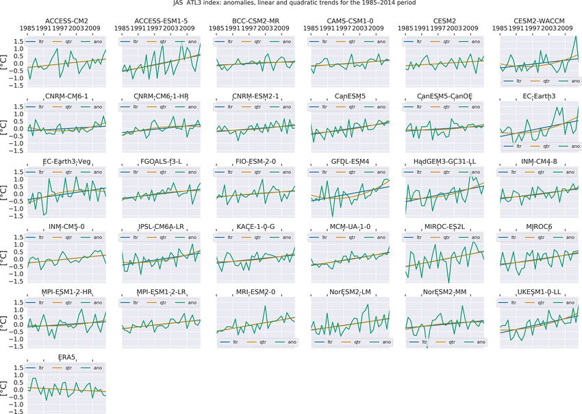
1

Supplement

S1   Supplement figures

Figure S1. SST indices of the Atlantic Niño: JAS mean of monthly SST anomalies averaged over the Atlantic Niño area, for the 1985–
2014 period (green curves). The linear (blue curves) and quadratic (orange curves) trends are superimposed on each panel. SST outputs from
CMIP6 historical simulations (30 GCMs) and the ERA5 reanalysis are considered.
2

Figure S2. Residuals of the detrended JAS ATL3 SST indices after removing the linear trend (blue curves) and the quadratic trend (orange
curves). The displayed 1985–2014 time series are from 30 CMIP6 models and ERA5.
3

Figure S3. JAS mean of monthly rainfall anomalies averaged over the Guinea Coast, for the 1985–2014 period (green curves). The linear
(blue curves) and quadratic (orange curves) trends are superimposed on each panel. Rainfall outputs from CMIP6 historical simulations
(30 GCMs) and the ERA5 reanalysis are considered.
4

Figure S4. Residuals of the detrended JAS Guinea Coast rainfall indices after removing the linear trend (blue curves) and the quadratic
trend (orange curves). The displayed 1985–2014 time series are from 30 CMIP6 models and ERA5.

Figure S5. Monthly rainfall anomalies of Guinea Coast regressed onto the JJA (a) and JAS (b) standardized ATL3 SST index over the
1985–2014 period. Outputs from 30 CMIP6 historical simulations and ERA5 are analyzed. Gray vertical bands indicate the SST season
considered in each case.

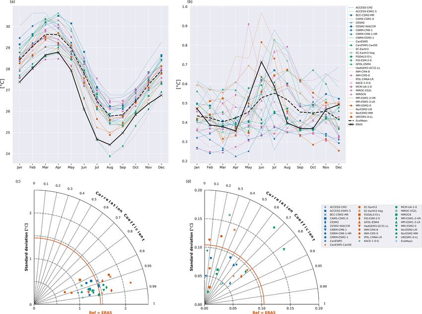
5

Figure S6. Annual cycle of the (a) rainfall intensity and (b) rainfall standard deviation in Guinea Coast. In (a) and (b), thick lines represent
the annual cycle of the multimodel ensemble mean (dashed line) and ERA5 (black line marked with a cross). The other lines represent the
annual cycle in each of the 30 GCMs. Taylor diagram of the (c) rainfall annual cycle, and (d) rainfall standard deviation annual cycle in the
GCB area, where ERA5 is chosen as the reference. The annual cycle is computed for the 1985–2014 period.

Figure S7. Mean biases (relative to ERA5) of the ensemble mean of 22 GCMs for the JAS SST (in colors), rainfall (in contours) and 10 m
horizontal wind (arrows) over 1985–2014. Among the 30 GCMs used in this study, these 22 models correspond to the ones that have the
10 m horizontal wind components for both the historical and SSP5–8.5 simulations.
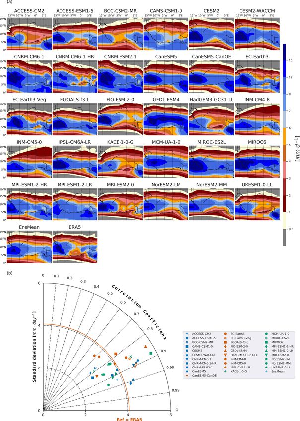
6

Figure S8. (a) 1985–2014 JAS rainfall mean in 30 GCMs and in ERA5. (b) Taylor diagram of the JAS rainfall mean over West Africa
(4–20◦ N), where the mean JAS rainfall spatial distributions in the models are compared to the one in ERA5.
7

Figure S9. Annual cycle of the (a) sea surface temperature and (b) sea surface temperature standard deviation in the ATL3 area. In (a)
and (b), thick lines represent the annual cycle of the multimodel ensemble mean (dashed line) and ERA5 (black line marked with a cross).
The other lines represent the annual cycle in each of the 30 GCMs. Taylor diagram of the (c) SST annual cycle and (d) SST standard deviation
annual cycle in the ATL3 area, where ERA5 is chosen as the reference. The annual cycle is computed for the 1985–2014 period.

Figure S10. Position in latitude of the maximum JAS rainfall associated with the JAS ATL3 SST index in the tropical Atlantic (zonal
average over 70◦ W and 10◦ E, blue boxplot) and West Africa (zonal average between 20◦ W and 10◦ E, dark gold boxplot). The boxplots
represent the distribution of the positions computed in each of the 30 models. The black line inside each box represents the median value of
the models, and the outliers are represented by the diamond-shaped symbols. The other horizontal lines represent the mean positions obtained
in the multi-model ensemble mean (green line) and ERA5 (dashed orange line).
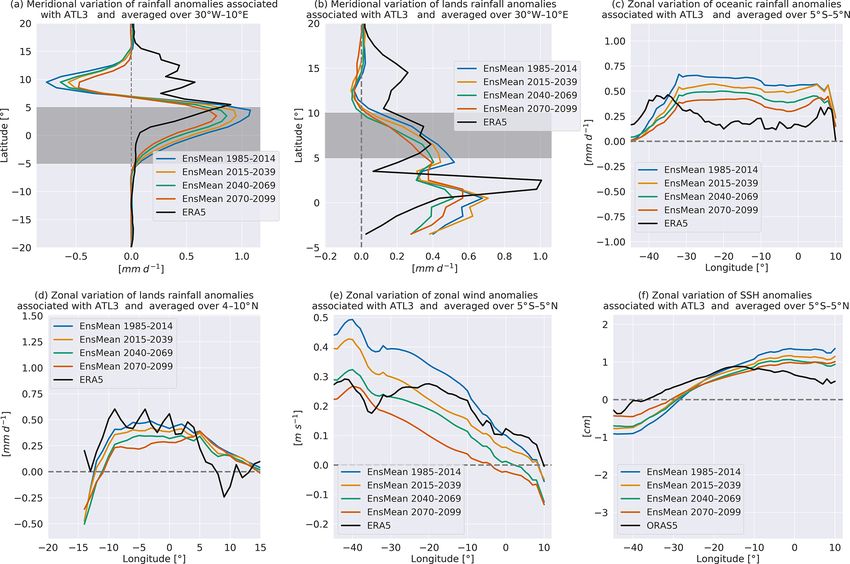
8

Figure S11. Sign-dependent average of the JAS rainfall regressed coefficients onto the standardized JAS ATL3 SST index over the Guinea
Coast box (a) and the equatorial Atlantic box (b) for the 30 GCMs over the present-day, near-term, mid-term and long-term periods. The
sign-dependent average value in ERA5 is computed for the 1985–2014 period.

Figure S12. Rainfall anomalies associated with the standardized JAS ATL3 SST index and averaged over 30 ◦ W and 10◦ E for oceanic
areas (a) and land areas (b). Gray bands in (a) and (b) represent the equatorial Atlantic and Guinea Coast regions, respectively. Zonal
variation of the JAS rainfall anomalies associated with the standardized JAS ATL3 SST index and averaged over the equatorial Atlantic (c)
and Guinea Coast regions (d). Zonal variation of the JAS 850 hPa zonal wind (e) and sea surface height anomalies (f) associated with the
standardized JAS ATL3 SST index and averaged over the equatorial Atlantic. In each panel, the solid black line represents ERA5 or ORAS5
for 1985–2014, and the other solid lines represent the ensemble mean of the 30 GCMs for the present and future periods.
9

Figure S13. Monthly stratified Niño3 index regressed onto the standardized JAS ATL3 SST index for different periods. The 1985–2014 pe-
riod is considered for ERA5 (black curve). The other curves correspond to the ensemble mean response of 30 CMIP6 models over four
different periods: 1985–2014, 2015–2039, 2040–2069 and 2070–2099.

Figure S14. JAS Niño3 index correlation with the JAS ATL3 SST index over four different periods. 30 CMIP6 models and the reanalysis
ERA5 are analyzed. Significant regression coefficients at 90 % confidence level (Student test) are highlighted with a black box.
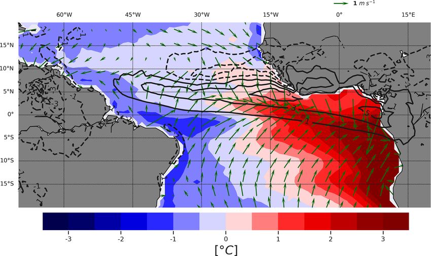
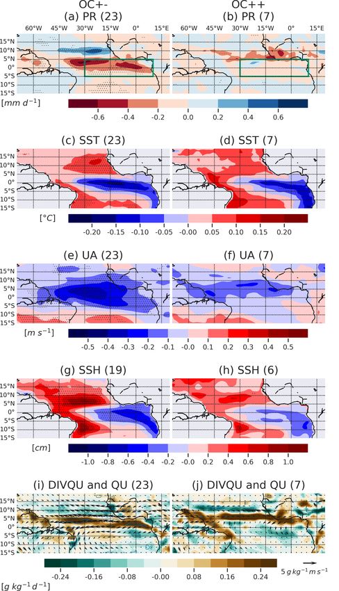
10

Figure S15. Long-term changes of the JAS rainfall (a, b), SST (c, d), 850 hPa zonal wind (e, f), sea surface height (g, h), moisture flux
(vectors) and moisture flux divergence (in colors) (i, j) regression patterns associated with the standardized JAS ATL3 SST index, relative
to the present-day climate (2070–2099 minus 1985–2014). Stippling in (a)–(h) and contours in (i)–(j) indicate areas where the mean change
(in colors) is significant at 95 % level according to a two-sided Welch t-test and where at least two thirds of the models agree on the sign of
the change. The number of models in each group is indicated in parentheses.
11

Figure S16. 1985–2014 regression maps of the JAS rainfall, SST, 850 hPa zonal and meridional moisture flux, DIV200/850, SSH, 850 hPa
moisture flux and moisture flux divergence anomalies onto the standardized JAS ATL3 SST index, for the GC+−, GC++, OC+−, OC++
and the 30 GCMs EnsMean groups. Stippling indicates areas where the regression coefficients are significant at 95 % confidence level for at
least 50 % of the models in each group, and where more than 80 % of the models agree on the sign of the regression coefficient. The number
of models in each group is indicated in parentheses.
12

Figure S17. 2070–2099 regression maps of the JAS rainfall, SST, 850 hPa zonal and meridional moisture flux, DIV200/850, SSH, 850 hPa
moisture flux and moisture flux divergence anomalies onto the standardized JAS ATL3 SST index, for the GC+−, GC++, OC+−, OC++
and the 30 GCMs EnsMean groups. Stippling indicates areas where the regression coefficients are significant at 95 % confidence level for at
least 50 % of the models in each group, and where more than 80 % of the models agree on the sign of the regression coefficient. The number
of models in each group is indicated in parentheses.
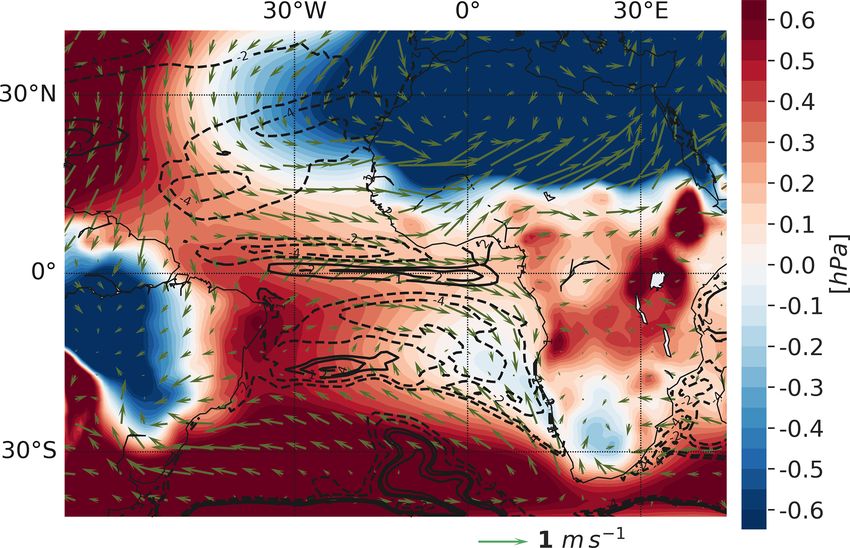
13

Figure S18. 1985–2014 (a, b) and 2070–2099 (c, d) regression maps of the JAS rainfall anomalies onto the standardized JAS ATL3 SST
index for the GC−− (a, c) and GC−+ (b, d) groups. Stippling indicates areas where the regression coefficients are significant at 95 %
confidence level for at least 50 % of the models in each group, and where more than 80 % of the models agree on the sign of the regression
coefficient. The number of models in each group is indicated in parentheses.

Figure S19. Long-term mean state change (2070–2099 minus 1985–2014) of the sea level pressure (in colors), 10 m horizontal wind (arrows)
and mixed layer depth (in contours in m). These changes are computed for the JAS season and averaged over 22 GCMs (Table 1).
14

S2    Supplement tables

Table S1. Multi-model averages of the JAS Guinea Coast rainfall, EAB rainfall, EAB SST, EAB 850 hPa zonal wind, EAB DIV200/850
and EAB SSH anomalies related to the JAS EAM in the GC++, GC+− and Ensmean groups.

                                                               GC++      GC+−     EnsMean   Unit
                               GCR             1985–2014          0.40     0.56      0.37   mm d−1
                                               2070–2099          0.49     0.10      0.24   mm d−1
                                               % of change       22.63   −83.01    −34.81
                               OCR             1985–2014         0.55      0.67      0.62   mm d−1
                                               2070–2099         0.42      0.33      0.40   mm d−1
                                               % of change     −22.93    −50.74    −35.95
                               SST             1985–2014         0.33      0.33      0.33   ◦C
                                               2070–2099         0.28      0.26      0.27   ◦C
                                               % of change     −15.22    −20.68    −18.50
                               UA              1985–2014         0.22      0.31      0.24   m s−1
                                               2070–2099         0.12      0.03      0.05   m s−1
                                               % of change     −44.18    −89.74    −79.44
                               DIV200/850      1985–2014         0.04      0.06      0.05   d−1
                                               2070–2099         0.03      0.02      0.03   d−1
                                               % of change     −32.88    −61.60    −49.81
                               ZOS             1985–2014         0.75      1.02      0.87   cm
                                               2070–2099         0.68      0.73      0.66   cm
                                               % of change      −9.40    −28.46    −23.42

Table S2. Models in the different categories for the 2015–2039 period.

     GC++               GC+−                   GC−+              GC−−                 OC+                OC−
     CAMS-CSM1-0        ACCESS-ESM1-5          CNRM-CM6-1        ACCESS-CM2           BCC-CSM2-MR        ACCESS-CM2
     CanESM5-CanOE      BCC-CSM2-MR            INM-CM4-8         HadGEM3-GC31-LL      CAMS-CSM1-0        ACCESS-ESM1-5
     EC-Earth3          CESM2                  KACE-1-0-G        INM-CM5-0            CESM2              CESM2-WACCM
     EC-Earth3-Veg      CESM2-WACCM                                                   CNRM-CM6-1         CNRM-CM6-1-HR
     FGOALS-f3-L        CNRM-CM6-1-HR                                                 CNRM-ESM2-1        CanESM5-CanOE
     GFDL-ESM4          CNRM-ESM2-1                                                   CanESM5            EC-Earth3
     MPI-ESM1-2-HR      CanESM5                                                       EC-Earth3-Veg      FGOALS-f3-L
     MRI-ESM2-0         FIO-ESM-2-0                                                   HadGEM3-GC31-LL    FIO-ESM-2-0
     NorESM2-LM         IPSL-CM6A-LR                                                  MIROC6             GFDL-ESM4
                        MCM-UA-1-0                                                    NorESM2-LM         INM-CM4-8
                        MIROC-ES2L                                                    UKESM1-0-LL        INM-CM5-0
                        MIROC6                                                                           IPSL-CM6A-LR
                        MPI-ESM1-2-LR                                                                    KACE-1-0-G
                        NorESM2-MM                                                                       MCM-UA-1-0
                        UKESM1-0-LL                                                                      MIROC-ES2L
                                                                                                         MPI-ESM1-2-HR
                                                                                                         MPI-ESM1-2-LR
                                                                                                         MRI-ESM2-0
                                                                                      NorESM2-MM
15
Table S3. Models in the different categories for the 2040–2069 period.
GC++ GC+− GC−+ GC−− OC+ OC−
CanESM5 ACCESS-ESM1-5 CNRM-CM6-1 ACCESS-CM2 CAMS-CSM1-0 ACCESS-CM2
EC-Earth3 BCC-CSM2-MR HadGEM3-GC31-LL INM-CM5-0 CESM2 ACCESS-ESM1-5
EC-Earth3-Veg CAMS-CSM1-0 INM-CM4-8 KACE-1-0-G CNRM-CM6-1 BCC-CSM2-MR
IPSL-CM6A-LR CESM2 CNRM-ESM2-1 CESM2-WACCM
MPI-ESM1-2-LR CESM2-WACCM EC-Earth3-Veg CNRM-CM6-1-HR
MRI-ESM2-0 CNRM-CM6-1-HR KACE-1-0-G CanESM5
CNRM-ESM2-1 MCM-UA-1-0 CanESM5-CanOE
CanESM5-CanOE MRI-ESM2-0 EC-Earth3
FGOALS-f3-L FGOALS-f3-L
FIO-ESM-2-0 FIO-ESM-2-0
GFDL-ESM4 GFDL-ESM4
MCM-UA-1-0 HadGEM3-GC31-LL
MIROC-ES2L INM-CM4-8
MIROC6 INM-CM5-0
MPI-ESM1-2-HR IPSL-CM6A-LR
NorESM2-LM MIROC-ES2L
NorESM2-MM MIROC6
UKESM1-0-LL MPI-ESM1-2-HR
MPI-ESM1-2-LR
NorESM2-LM
NorESM2-MM
UKESM1-0-LL
Table S4. Models in the different categories for the 2070–2099 period.
GC++ GC+− GC−+ GC−− OC+ OC−
ACCESS-ESM1-5 CAMS-CSM1-0 CNRM-CM6-1 ACCESS-CM2 BCC-CSM2-MR ACCESS-CM2
BCC-CSM2-MR CESM2 HadGEM3-GC31-LL KACE-1-0-G CESM2 ACCESS-ESM1-5
CanESM5 CESM2-WACCM INM-CM4-8 CNRM-CM6-1 CAMS-CSM1-0
CanESM5-CanOE CNRM-CM6-1-HR INM-CM5-0 CanESM5 CESM2-WACCM
EC-Earth3 CNRM-ESM2-1 MIROC6 CNRM-CM6-1-HR
EC-Earth3-Veg FGOALS-f3-L MRI-ESM2-0 CNRM-ESM2-1
GFDL-ESM4 FIO-ESM-2-0 NorESM2-MM CanESM5-CanOE
IPSL-CM6A-LR MIROC-ES2L EC-Earth3
MCM-UA-1-0 MIROC6 EC-Earth3-Veg
MPI-ESM1-2-LR MPI-ESM1-2-HR FGOALS-f3-L
MRI-ESM2-0 NorESM2-LM FIO-ESM-2-0
UKESM1-0-LL NorESM2-MM GFDL-ESM4
HadGEM3-GC31-LL
INM-CM4-8
INM-CM5-0
IPSL-CM6A-LR
KACE-1-0-G
MCM-UA-1-0
MIROC-ES2L
MPI-ESM1-2-HR
MPI-ESM1-2-LR
NorESM2-LM
UKESM1-0-LLYou can also read