SHCal20 SOUTHERN HEMISPHERE CALIBRATION, 0-55,000 YEARS CAL BP
←
→
Page content transcription
If your browser does not render page correctly, please read the page content below
Radiocarbon, Vol 62, Nr 4, 2020, p 759–778                                    DOI:10.1017/RDC.2020.59
               © 2020 by the Arizona Board of Regents on behalf of the University of Arizona. This is an Open Access
               article, distributed under the terms of the Creative Commons Attribution licence (http://creativecommons.
               org/licenses/by/4.0/), which permits unrestricted re-use, distribution, and reproduction in any medium,
               provided the original work is properly cited.

               SHCal20 SOUTHERN HEMISPHERE CALIBRATION, 0–55,000 YEARS CAL BP
               Alan G Hogg1,2* • Timothy J Heaton3 • Quan Hua4 • Jonathan G Palmer2,5                                                         •
               Chris SM Turney2,5 • John Southon6 • Alex Bayliss7 • Paul G Blackwell3 •
               Gretel Boswijk8 • Christopher Bronk Ramsey9 • Charlotte Pearson10 •
               Fiona Petchey1,11 • Paula Reimer12 • Ron Reimer12 • Lukas Wacker13
               1
                Waikato Radiocarbon Laboratory, University of Waikato, Private Bag 3105, Hamilton, New Zealand
               2
                ARC Centre of Excellence for Australian Biodiversity and Heritage, School of Biological, Earth and Environmental
               Sciences, University of New South Wales, Sydney, NSW 2052, Australia
               3
                School of Mathematics and Statistics, University of Sheffield, Sheffield S3 7RH, UK
               4
                Australian Nuclear Science and Technology Organisation, Locked Bag 2001, Kirrawee DC, NSW 2232, Australia
               5
                Chronos 14Carbon-Cycle Facility and Changing Earth, University of New South Wales, Sydney, NSW 2052, Australia
               6
                Department of Earth System Science, University of California, Irvine, CA 92697-3100, USA
               7
                Historic England, 4th Floor, Cannon Bridge House, 25 Dowgate Hill, London, EC4R 2YA, UK
               8
                School of Environment, University of Auckland, New Zealand
               9
                Research Laboratory for Archaeology and the History of Art, University of Oxford, 1 South Parks Road, Oxford
               OX1 3TG, UK
               10
                 The Laboratory of Tree-Ring Research, University of Arizona, Tucson, AZ 85721-0400, USA
               11
                 ARC Centre of Excellence for Australian Biodiversity and Heritage, College of Arts, Society and Education, James
               Cook University, PO Box 6811, Cairns, Queensland 4870, Australia
               12
                 Centre for Climate, the Environment & Chronology (14CHRONO), School of Natural and Built Environment,
               Queen’s University Belfast, Belfast BT7 1NN, UK
               13
                 Laboratory of Ion Beam Physics, HPK, H29, Otto-Stern-Weg 5, CH-8093 Zürich, Switzerland

               ABSTRACT. Early researchers of radiocarbon levels in Southern Hemisphere tree rings identified a variable North-
               South hemispheric offset, necessitating construction of a separate radiocarbon calibration curve for the South. We
               present here SHCal20, a revised calibration curve from 0–55,000 cal BP, based upon SHCal13 and fortified by the
               addition of 14 new tree-ring data sets in the 2140–0, 3520–3453, 3608–3590 and 13,140–11,375 cal BP time
               intervals. We detail the statistical approaches used for curve construction and present recommendations for the use
               of the Northern Hemisphere curve (IntCal20), the Southern Hemisphere curve (SHCal20) and suggest where
               application of an equal mixture of the curves might be more appropriate. Using our Bayesian spline with errors-
               in-variables methodology, and based upon a comparison of Southern Hemisphere tree-ring data compared with
               contemporaneous Northern Hemisphere data, we estimate the mean Southern Hemisphere offset to be 36 ± 27 14C
               yrs older.

               KEYWORDS: carbon cycle, Inter-Tropical Convergence Zone (ITCZ), interhemispheric gradient (IHG), North-South
               hemispheric offset, Southern Ocean, tropical and sub-tropical radiocarbon calibration.

               1. HISTORY OF SOUTHERN HEMISPHERE CALIBRATION
               The conversion of terrestrial radiocarbon (14C) ages into calendar time requires a calibration
               curve that accurately reflects past atmospheric 14C levels. Tree rings offer unsurpassed accuracy
               and resolution if derived from a replicated tree-ring chronology and if adequately pretreated, so
               that the dated fraction faithfully captures atmospheric 14C concentrations at the time of
               growth, unaffected by variable lignin contents or species-specific differences (McCormac
               et al. 1998a).

               Whilst a major focus of the radiocarbon community has been the calibration of the timescale,
               early work soon demonstrated there was an offset in atmospheric 14C concentrations between
               the hemispheres. Some of the earliest measurements of Southern Hemisphere (SH) tree rings

               *Corresponding author. Email: alan.hogg@waikato.ac.nz.

Downloaded from https://www.cambridge.org/core. IP address: 46.4.80.155, on 17 Dec 2021 at 23:18:57, subject to the Cambridge Core terms of use,
available at https://www.cambridge.org/core/terms. https://doi.org/10.1017/RDC.2020.59
760 A G Hogg et al.

               indicated depleted 14C levels with SH tree rings giving older values compared to
               contemporaneous tree rings from the Northern Hemisphere (NH). This was probably a
               result of higher sea-air 14CO2 flux from the larger expanse of SH oceans (Lerman et al.
               1970; Rodgers et al. 2011). Lerman et al. (1969, 1970) measured a North-South (N-S)
               hemispheric offset of ~ 36–42 14C yrs and Vogel et al. (1986, 1993) measured additional
               Netherlands/South Africa sample pairs and obtained a value of 41 ± 5 14C yrs†. Vogel et al.
               (1993) recommended using this constant to create a calibration curve for SH mid-latitudes,
               based upon the data of Stuiver and Pearson (1993) for the NH.

               Subsequently, paired decadal measurements made from contemporaneous British oak
               (Quercus petraea) and New Zealand (NZ) cedar (Libocedrus bidwillii) or silver pine
               (Manoao colensoi) tree rings from 1000–0 cal BP by Queen’s University Belfast (identifier
               UB) and Waikato University (identifier Wk), showed there were differences between the
               structural forms of the radiocarbon calibration curves for each hemisphere. They
               demonstrated that the N-S offset was not constant but varied with time, with a periodicity
               of approximately 130 cal yrs, and amplitudes ranging from 8–80 14C yrs (McCormac et al.
               1998a, 1998b; Hogg et al. 2002). Building on this work, McCormac et al. (2002) published
               the first iteration of SHCal (SHCal02) covering the interval 1000–100 cal BP, compiled
               from data sets derived from NZ (Wk, UB; McCormac et al. 1998a, 1998b; Hogg et al.
               2002), Chile (Quaternary Isotope Lab, identifier QL; Stuiver and Braziunus 1998),
               Tasmania (QL; Stuiver and Braziunus 1998) and South Africa (Pretoria, identifier Pta;
               Vogel et al. 1993). The combined SH data sets showed a mean offset of 41 ± 14 14C yrs for
               the interval 1000–100 cal BP and in the absence of additional measured SH data, the
               authors recommended this value be applied to IntCal98 (Stuiver et al. 1998) for the period
               outside this range. The SH calibration was extended to 11,000 cal BP by McCormac et al.
               (2004) using the same random walk model and parameters as for IntCal04 (Reimer et al.
               2004, Buck and Blackwell 2004). SHCal04 contained the SHCal02 data sets and IntCal04
               data with a modeled offset beyond the range of the SH measurements. The modeled offset
               ranged from 55 to 58 14C yrs with uncertainties increasing from ±7.9 14C yrs at 1000 cal BP
               to ±25 14C yrs at 11,000 cal BP.

               In parallel with the above studies, Hua et al. (2004a) obtained 16 decadal sample pairs
               (Australian Nuclear Science & Technology Organisation, identifier OZ) from Tasmania
               (Huon pine, Lagarostrobos franklinii) and Thailand (Pinus merkusii) for the interval
               325–175 cal BP to investigate the 14C content of the atmosphere sampled by tropical
               trees. The mean offset between Tasmania (older) and Thailand was 30 ± 8 14C yrs.
               Further back in time, Hua et al. (2009) analysed 134 tree-ring samples (OZ) from four
               Younger Dryas (YD)-age Tasmanian Huon pine subfossil logs (SRT-779, -781, -782, -783)
               extracted from alluvial sediments along Stanley River in Northwest Tasmania (Australia).
               Ring-width measurements, supplemented by 14C wiggle-matching against IntCal04 data
               (utilizing a 40 14C-yrs constant N-S offset) produced a 617-yrs-long floating chronology,
               spanning the calendar age interval of 12,679–12,072 (± 11) cal BP. Zimmerman et al. (2010)
               obtained new decadal measurements (Center for AMS, identifier CAMS) from a Huon pine
               tree-ring series for the interval 2115–855 cal BP. However, Hogg et al. (2011) obtained data
               (Wk) for a similar interval from NZ kauri (Agathis australis: 2145–955 cal BP) tree-ring
               series (Boswijk et al. 2014) and suggested some of the equivalent Huon pine data had
               underestimated uncertainties, with some data points (1205–1075 cal BP) that could be too

               †
                All uncertainties given are 1σ unless stated otherwise.

Downloaded from https://www.cambridge.org/core. IP address: 46.4.80.155, on 17 Dec 2021 at 23:18:57, subject to the Cambridge Core terms of use, available at
https://www.cambridge.org/core/terms. https://doi.org/10.1017/RDC.2020.59
SHCal20 Southern Hemisphere Calibration 761
young. This was confirmed by re-measurement of nine Huon pine decadal samples (Wk) from the
interval 1175–1095 cal BP (Hogg et al. 2013a).
Building on the above studies and new datasets from the NH, the 2013 iteration of the SH curve
was extended from 0 to 50,000 cal BP (Hogg et al. 2013b). The resulting SHCal13 was a
compilation of the SH data sets described above, and based upon IntCal13 data (Reimer
et al. 2013), corrected for a N-S offset, beyond the range of the measured data sets. The
calibration curve was constructed using a Markov Chain Monte Carlo (MCMC)
implementation of the random walk model, with transitional regions where the variance
depends upon the measured (SH data) and modeled (IntCal13 data adjusted by the N-S
offset) data sets (Heaton et al. 2009; Niu et al. 2013).
There are some aspects of SHCal13 that have potentially important implications for SHCal20:
1. The value of 129 ± 14 BP from Pretoria (identifier Pta) for 100 cal BP (1850 CE) that was
used in SHCal04 and SHCal13 is incorrect. The correct value of 155 ± 11 BP (Hogg et al.
2019) is used in SHCal20.
2. Of the four YD-age subfossil Huon pine 14C data sets in Hua et al. (2009), only SRT-779
agreed closely with contemporaneous YD-age subfossil New Zealand kauri (see further
details below). For this reason, the other three Huon pine data sets (SRT-781, -782, and
-783) have been omitted from SHCal20.
2. NEW SOUTHERN HEMISPHERE DATA SETS
2.1 High-resolution data relating to the 774 and 993 CE cosmic events
Miyake et al. (2012, 2013) discovered two large and rapid increases in atmospheric
14
C concentration (Δ14C) from Japanese tree rings dated to 1176/5 cal BP (774/5 CE)
and 957/6 cal BP (993/4 CE). Corresponding anomalous 10Be and 36Cl events recorded
in ice cores (Mekhaldi et al. 2015) suggest extreme fluxes from high-energy solar particles
were responsible. The NH expression of these events has been detailed in several studies (see
Büntgen et al. 2018 and references therein). Güttler et al. (2015) measured Δ14C levels in NZ
kauri, showing their global nature. Annual or biennial SH Δ14C data from seven tree-ring
series, six relating to the 774 CE event (four from NZ and one each from Chile and
Tasmania) and one to the 993 CE event (NZ)—Table 1 are available from the Büntgen et al.
(2018) study (ETH/AMS facility, identifier ETH, alpha-cellulose). They calculated offsets
to contemporaneous NH data of ~30 14C yrs (in terms of Δ14C, these offsets equate to
4.0 ± 0.4‰ in 774 CE and 3.5 ± 0.7‰ in 993 CE). These data are available from the
SHCal database (http://intcal.org/shcal20/— datasets 9-1, 9-2, 9-3, 9-4, 9-5, 9-6). The
high-resolution SH data compare well with existing SH decadal data (Figures 1A and 1B).
2.2 New 450–0 cal BP data sets
Four new data sets in the interval 450–0 cal BP have been included in SHCal20 (see Table 2).
Data set 3-7 contains 22 Wk decadal solvent-extracted alpha-cellulose high precision
radiometric analyses spanning the interval 1725–1935 CE and first given in McCormac
et al. (1998a). This group of analyses was accidentally omitted from SHCal04 and SHCal13
but is included in SHCal20.
Downloaded from https://www.cambridge.org/core. IP address: 46.4.80.155, on 17 Dec 2021 at 23:18:57, subject to the Cambridge Core terms of use, available at
https://www.cambridge.org/core/terms. https://doi.org/10.1017/RDC.2020.59762 A G Hogg et al.
Table 1 Summary of new high-resolution SH tree-ring chronologies/data sets including the
time span, block interval (number of yrs [i.e. rings] per analysis) and total number of analyses (N).
From Büntgen et al. (2018).
Block
Series IDa Location Species/Lat.,long. Time span interval N
9-1. Dargaville, NZ Agathis australis 950–960 CE 0.5-1 24
DAR01 35°55’S, 173°48’E 1000–990 cal BP
(HAR010a)
9-1. Dargaville, NZ Agathis australis 770–780 CE 0.5-1 24
DAR01 35°55’S, 173°48’E 1180–1170 cal
(HAR010a) BP
9-2. Dargaville, NZ Agathis australis 770–780 CE 1 11
DAR06 35°55’S, 173°48’E 1180–1170 cal
(HAL025a) BP
9-3. Dargaville, NZ Agathis australis 1770–780 CE 1 11
DAR07 35°55’S, 173°48’E 1180–1170 cal
(HAL025b) BP
9-4. Moana, NZ Manoao colensoi 770–780 CE 1 11
NEW01 42°30’S, 171°38’E 1180–1170 cal
(LC122) BP
9-5. El Asiento, Chile Austrocedrus chilensis 770–780 CE 1 11
PAT02 32°39’S, 70°49’W 1180–1170 cal
(ELA1-2) BP
9-6. Stanley R., Lagarostrobos 770–780 CE 1 11
TAS01 Tasmania franklinii 1180–1170 cal
(SRT554A) 41°45’S, 145°14’E BP
a
Series numbers 9-1 to 9-6 correspond with “Set No.” and “Division” in SHCal database (http://intcal.org/shcal20).
Data sets 3-8 and 3-9 are composed from Wk decadal alpha-cellulose AMS analyses spanning
the interval 1705–1945 CE and published in Turney et al. (2016). This publication also contained
complementary data from Lake Tay (Western Australia) and Campbell Island (NZ). The Lake
Tay data set was not considered for SHCal20 because of suspicions that the very high resin
content characteristic of the Callitris columellaris trees may have resulted in translocation
of 14C across ring boundaries. The Campbell Island Dracophyllum longifolium data, also
omitted, was systematically older than contemporaneous measurements from mid-latitude
SH locations, probably as a result of its high latitude Southern Ocean location. See Hogg et al.
(2019) for a discussion of both the Lake Tay and Campbell Island data sets. Data set 3-10
contains duplicated Wk five-ring alpha-cellulose AMS analyses spanning the interval 1652–1827
CE and published in Hogg et al. (2019).
Hogg et al. (2019) presented a new Bayesian spline method for calibration curve construction
(see below) and tested it on 11 SH data sets. The four new data sets presented here had relative
offsets from the mean of ~ 6 to –6 14C yrs indicating their suitability for inclusion in SHCal20.
2.3 New 3608–3453 cal BP data sets
Two new single tree ring data sets in the interval 3608–3453 cal BP have been included in
SHCal20 (see Table 3). Data set 7-1 contains 16 University of Arizona AMS Facility
Downloaded from https://www.cambridge.org/core. IP address: 46.4.80.155, on 17 Dec 2021 at 23:18:57, subject to the Cambridge Core terms of use, available at
https://www.cambridge.org/core/terms. https://doi.org/10.1017/RDC.2020.59SHCal20 Southern Hemisphere Calibration 763
A
1400
3-1. ORS872, TKP07
1380 3-6. SRT440
9-1. DAR01
1360 9-2. DAR06
9-3. DAR07
1340 9-4. NEW01
Radiocarbon determination (BP)
9-5. PAT02
9-6. TAS01
1320
SHCal13
1300
1280
1260
1240
1220
1200
1180
1160
1180 1175 1170 1165
Calendar age (calBP)
Figure 1A Southern Hemisphere tree-ring 14C data relating to the 774 CE event. Tree-
ring series include: 3-1 (Wk, Manoao colensoi, Oroko Swamp, NZ and Libocedrus bidwillii,
Takapari Forest Park, NZ); 3-6 (Wk, Lagarostrobos franklinii, Stanley River, Tasmania,
Australia); 9-1, 9-2, 9-3 (ETH, Agathis australis, Dargaville, NZ); 9-4 (ETH, Manoao
colensoi, Moana, NZ); 9-5 (ETH, Austrocedrus chilensis, El Asiento, Chile); 9-6 (ETH,
Lagarostrobos franklinii, Stanley River, Tasmania, Australia).
analyses (identifier AA) spanning the interval 3608–3590 cal BP and 65 AA analyses spanning
3520–3453 cal BP. Pearson et al. (2020 in this issue) compare a sub-set of these data with single
year measurements (AA) from Irish oak and North American bristlecone pine, and provide
additional fine scale information on the N-S offset during this period.
The two new AA data sets are plotted with SHCal13 in Figure 2.
2.4 New Younger Dryas-age measurements
Hogg et al. (2016a, 2016b) presented a floating 14C chronology containing 1022 measurements
from NZ kauri trees spanning the interval ~11,285–9990 14C yrs BP (mean 1σ uncertainty =
±28 14C yrs). The kauri trees were located in Northland, at Towai (series name 8-1, CRW003)
and Dargaville (series name 8-2, FIN11). The Towai decadal samples (~11,285–10,070 14C BP)
were derived from a well replicated and securely cross-matched tree-ring chronology (1451
rings, 91 radial strips derived from 37 trees with an average cross-correlation coefficient
between all series of 0.71, Palmer et al. 2016). The 778 analyses were determined principally
by University of California, Irvine (identifier UCI, holo-cellulose, AMS), Wk (alpha-
cellulose, high precision liquid scintillation spectroscopy) and Oxford University (identifier
OxA, alpha-cellulose, AMS) with a few additional analyses by ETH (alpha-cellulose, AMS)
and University of Heidelberg (identifier Hd, holo-cellulose, Gas Proportional Counting - GPC).
The Dargaville decadal samples (~10,305–9990 14C yrs BP) were obtained from a single tree
(FIN11, two measured radii, estimated 533 rings), with the 244 analyses undertaken by UCI
Downloaded from https://www.cambridge.org/core. IP address: 46.4.80.155, on 17 Dec 2021 at 23:18:57, subject to the Cambridge Core terms of use, available at
https://www.cambridge.org/core/terms. https://doi.org/10.1017/RDC.2020.59764 A G Hogg et al.
B
1200
3-1. ORS872, TKP07
1180 3-6. SRT440
4-1. ORS872
6-2. SRT44
1160 9-1. DAR01
SHCal13
Radiocarbon determination (BP)
1140
1120
1100
1080
1060
1040
1020
1000
980 975 970 965 960 955 950 945 940 935 930 925
Calendar age (calBP)
Figure 1B Southern Hemisphere tree-ring 14C data relating to the 993 CE event. Tree-
ring series include: 3-1 (Wk, Manoao colensoi, Oroko Swamp, NZ and Libocedrus
bidwillii, Takapari Forest Park, NZ); 3-6 (Wk, Lagarostrobos franklinii, Stanley River,
Tasmania, Australia); 4-1 (UB, Manoao colensoi, Oroko Swamp, NZ); 6-2 (CAMS,
Lagarostrobos franklinii, Stanley River, Tasmania, Australia); 9-1 (ETH, Agathis
australis, Dargaville, NZ).
(holo-cellulose, AMS) and Wk (alpha-cellulose, predominantly high precision liquid scintillation
spectroscopy).
The Towai and Dargaville 14C data sets were wiggle-matched against contemporaneous NH
data contained within IntCal13, being careful to avoid aberrant sections of the curve (see Hogg
et al. 2016a for details), returning calendar age estimates of ~13,134–11,695 cal BP (Towai) and
~11,870–11,367 cal BP (Dargaville). More recent unpublished higher resolution NH pine
(Pinus sylvestris) and NZ kauri measurements by ETH have indicated that the Towai kauri
YD 14C data set should be shifted towards older ages by 10 ± 3 cal yrs resulting in a final
calendar age range of ~13,144–11,705 ± 3 cal BP (Sookdeo et al. 2019 in this issue, 2020).
This shift also affects the Dargaville series, with an adjusted calendar age range of
~11,880–11,377 ± 5 cal BP. Both Towai and Dargaville data sets have been included in
SHCal20 on the basis of a recent decision made by the IntCal Working Group to accept
wiggle-matched data from pre-Holocene floating trees.
The four YD-age Huon pine samples analysed by Hua et al. (2009) were compared with the
Towai kauri series by Hogg et al. (2016a). The four trees could not be cross-matched by
dendrochronology alone and required additional linking by 14C wiggle-matching (Hua
et al., 2009); of the four, only SRT-779 agreed closely with the well-replicated Towai
chronology (n = 24; Acomb = 126.4%; An = 14.4%. χ2 -test: df = 23 T = 15.018 (5% 35.173) -
see Hogg et al. 2016a for model details) and is retained for SHCal20. For more information
on the chronological issues associated with some of the YD-age Huon pine 14C series and
ultimately their exclusion from SHCal20, please refer to Hogg et al. (2016a, 2016b).
Downloaded from https://www.cambridge.org/core. IP address: 46.4.80.155, on 17 Dec 2021 at 23:18:57, subject to the Cambridge Core terms of use, available at
https://www.cambridge.org/core/terms. https://doi.org/10.1017/RDC.2020.59https://www.cambridge.org/core/terms. https://doi.org/10.1017/RDC.2020.59
Downloaded from https://www.cambridge.org/core. IP address: 46.4.80.155, on 17 Dec 2021 at 23:18:57, subject to the Cambridge Core terms of use, available at
Table 2 Summary of new 450–0 cal BP SH tree-ring chronologies/data sets showing the time span, block interval (number of yrs [i.e. rings]
per analysis) and total number of analyses (N). Dating methods: HPLSC—high precision liquid scintillation counting; AMS—accelerator
mass spectrometry.
Time span
ID Location Species/Lat.,long. (mid-points) Block interval N Notes
3-7. Hihitahi Forest Libocedrus bidwillii 1725–1935 CE 10 22 McCormac et al. (1998a)
H4702 Park, NZ 39°32’S, 175°44’ 224.5–14.5 cal BP HPLSC
solv. extr. α-cellulose
3-8. Hihitahi Forest Libocedrus bidwillii 1705–1945 CE 10 45 Turney et al. (2016)
H4702, TKP144# Park, NZ 39°32’S, 175°44’ 244.5–4.5 cal BP AMS
SHCal20 Southern Hemisphere Calibration 765
α-cellulose
3-9. DBY225^ Doughboy Bay, Halocarpus biformis 1705–1945 CE 10 45 Turney et al. (2016)
Stewart Isl., 47°01’S, 167°42’E 244.5–4.5 cal BP AMS
NZ α-cellulose
3-10. SPC002 Auckland, NZ Agathis australis‡ 1652–1827 CE 5 72 Hogg et al. (2017, 2019)
298–123 cal BP AMS¶
solv. extr. α- cellulose
^1915–1945 decades given preliminary multiple solvent (acetone) extractions.
¶duplicate analyses.
#1931–1950 decades from Takapari FP (40°04’S, 175°59’E).
solv. extr. = solvent (acetone) extracted.
‡
kauri derived from the upper North Island of NZ but exact geographic location unknown.766 A G Hogg et al.
Table 3 Summary of new 3608–3453 cal BP SH tree-ring chronologies/data sets showing
the time span, block interval (number of yrs [i.e. rings] per analysis) and total number of
analyses (N).
Time span Block
ID Location Species/Lat.,long. (mid-points) interval N Notes
7-1. Gibsons Agathis australis 3608–3590 cal 1 16 Pearson et al.
GIB102 Farm 35°54’S, 173°48’E BP (2020 in this
Dargaville, 3520–3453 cal 1 65 issue), AMS,
NZ BP holo-cellulose
3500
7-1
SHCal13
3450
Radiocarbon determination (BP)
3400
3350
3300
3250
3200
3650 3600 3550 3500 3450 3400
Calendar age (calBP)
Figure 2 New single-ring 14C data sets (7-1) in the interval 3608–3453 cal BP. Series 7-1
(AA, Agathis australis, Dargaville NZ).
The YD-age data sets included in SHCal20 are shown graphically in Figure 3. The new YD
measurements refine the shape of the SH atmospheric curve from ~13,100–11,400 cal BP.
Hogg et al. (2016a) showed that the 14C calibration curve IntCal13, and as a consequence
SHCal13, was clearly too young from ~12,200–11,900 cal BP. This time interval had
previously been occupied by an incorrectly linked larch tree-ring series from Ollon,
Switzerland (Ollon505, also termed VOD505, Hogg et al. 2013c). They also showed that
the YD-B chronology was incorrectly linked by dendrochronology to NH Holocene data
and this caused the ~10,400 BP 14C plateau in IntCal13 and SHCal13 to be ~5 decades too
short, thus shifting the two 14C peaks seen at around 12,500 cal BP towards older calendar
ages by about 50 cal yrs. This finding has recently been confirmed with new
dendrochronological and 14C measurements on NH trees (Sookdeo et al. 2019, 2020).
Downloaded from https://www.cambridge.org/core. IP address: 46.4.80.155, on 17 Dec 2021 at 23:18:57, subject to the Cambridge Core terms of use, available at
https://www.cambridge.org/core/terms. https://doi.org/10.1017/RDC.2020.59SHCal20 Southern Hemisphere Calibration 767
8-1 CRW003
8-2 FIN11
11,200 5-1 WM SRT779
SHCal13
11,000
Radiocarbon determination (BP)
10,800
10,600
10,400
10,200
10,000
13,000 12,500 12,000 11,500
Calendar age (calBP)
Figure 3 Southern Hemisphere YD-age tree-ring 14C data sets. Tree-ring series include:
8-1 (UCI, Wk and OxA, Agathis australis, Towai, NZ; 8-2 (UCI and Wk, Agathis australis,
Dargaville NZ); 5-1 (OZ, Lagarostrobos franklinii, Stanley River, Tasmania, Australia).
3. CALIBRATION CURVE CONSTRUCTION
We would ideally wish to create a complete, annually resolved, SHCal20 calibration curve
based solely upon direct SH observations and without requiring any modeling assumptions
about the nature of the N-S hemispheric offset to be made. Such a curve would be entirely
independent from the NH IntCal20 curve (Reimer et al. 2020 in this issue). With our new
and existing datasets this is achievable in four distinct time periods: those covering the SH
trees dated by dendrochronology of approximately 2140–0, 3520–3453, and 3608–3590 cal
BP; and that covering the floating SH trees of approximately 13,140–11,375 cal BP.
However outside these time periods we are lacking direct SH observations, and so in order
to create the SHCal curve, we will need to include information from the corresponding NH
IntCal20 curve. This requires us to make a simple statistical model of the N-S atmospheric
radiocarbon offset to transfer information from the NH data.
We aim to provide a construction method where, for the four time periods listed above with
dense SH data, the SHCal20 curve is the exact curve one would obtain using only that SH data.
These SH-data-based sections of curve are then used to learn about the nature of the N-S
hemispheric offset and extrapolate to extend SHCal20 over the complete 0–55 cal kBP
(thousands of calibrated years before present) time range. The construction process is
shown in Figure 4. The concept is similar to that used for SHCal13 although the new
SHCal20 methodology incorporates and estimates the N-S offset, and hence the final SH
calibration curve, more rigorously.
3.1 Creating a curve where we have SH observations
We commence by creating a preliminary SH calibration curve based only on the available SH
data using the same Bayesian spline with errors-in-variables methodology of IntCal20; see
Downloaded from https://www.cambridge.org/core. IP address: 46.4.80.155, on 17 Dec 2021 at 23:18:57, subject to the Cambridge Core terms of use, available at
https://www.cambridge.org/core/terms. https://doi.org/10.1017/RDC.2020.59768 A G Hogg et al.
A
B C
D E
F
Figure 4 A step-by-step illustration of SHCal20 curve construction. Panel A: The SH
14
C observations covering the four distinct time periods where direct measurements are
available. We initially fit a Bayesian spline to this observed SH 14C data. In the periods
where we have sufficient direct SH observations, this spline fit is SHCal20; outside these
times, in periods where we not have direct SH observations and this initial spline is not
informative, we instead base SHCal20 on importing information from the NH by
modeling the N-S hemispheric offset. Panel B: A zoomed-in section with a posterior
realization of the initial spline fitted to the SH 14C observations, the rug indicates the
knot locations. Where we do not have direct SH observations this initial fitted spline is
deleted (red dashed line) leaving an incomplete part SH-realization (red solid line). Panel
C: The incomplete part SH-realization (red solid line) is paired with a complete 0–55 cal
kBP NH IntCal20 spline realization (blue solid line). Panel D: In periods where we have
direct SH data the offset between the selected part SH- and complete NH- spline
realizations is calculated (black solid line) and extended to the missing periods (green
solid line) by modeling, conditional on the black calculated values, as an AR(1) process.
Panel E: The completed, AR(1)-simulated, offset is added back to the NH-realization
providing a completed 0–55 cal kBP SH-realization (red solid line). Due to construction,
in periods where SH data is available this completed SH-realization will be identical to
the initial part SH-realization. Panel F: This process is repeated with multiple (part
SH- and complete NH-) spline realizations to provide an ensemble of AR(1)-completed
SH-realizations which are summarized to provide the SHCal20 curve. (Please see
electronic version for color figures.)
Downloaded from https://www.cambridge.org/core. IP address: 46.4.80.155, on 17 Dec 2021 at 23:18:57, subject to the Cambridge Core terms of use, available at
https://www.cambridge.org/core/terms. https://doi.org/10.1017/RDC.2020.59SHCal20 Southern Hemisphere Calibration 769
Histogram of Posterior for τ with square root scaled additive error ηi~N(0, τ2f(θi))
SIRI−based Prior
3000
Density
1000
0
0.000 0.002 0.004 0.006 0.008 0.010
τ
Figure 5 Histogram of the posterior for τ, the level of over-dispersion in the SHCal20
data. We model Fi , the observed value of F14C in (annual) datum i with calendar age θi ,
as Fi f θi ϵi
ηi . Here
f θi is the underlying atmospheric F14C level
at θi cal BP
in the SH; ϵi N 0; σ 2i the laboratory reported uncertainty; and ηi N 0; τ 2 f θi the
over-dispersion used to model any potential further additional variability seen in the
SHCal20 data. Note that, p as for IntCal20, our model for this over-dispersion/additional
variability scales with f θi , the square root of F14C. We also show the SIRI-based
prior in red. As expected, this SIRI-based prior on the level of over-dispersion is larger
than our posterior due to the screening criteria for SHCal20 data. The posterior
estimate is dominated by the SHCal20 data rather than the prior.
Heaton et al. (2020 in this issue) for further details. For the three distinct time periods covered
by the observed SH trees dated by dendrochronology (approximately 2140–0, 3520–3453,
3608–3590 cal BP) we select the same knots for our spline, both in terms of number and
location, as used in IntCal20. This includes the specific, additional knots placed around
774/5 CE and 993/4 CE used to enable representation of the rapid Miyake “cosmic” events
(Miyake et al. 2012, 2013). This matched knot selection with the NH IntCal20 curve
enables equitable comparisons on the N-S hemispheric offset to be made and, since the
density of the SH data is lower than the density of the data from the NH, is sufficient for
us to capture the detail within the available SH 14C observations. For the floating SH tree
rings (approximately 13,140–11,375 cal BP) we use the same number of knots as in the
corresponding section of the IntCal20 curve but space them evenly over the interval. Such
a placement allows the Bayesian method to explore the exact calendar location of these
floating trees equitably—an uneven knot spacing introduces bias as the method will tend to
align the trees so that wiggles in the underlying levels of 14C fit with higher knot density
(Heaton et al. 2020 in this issue). Outside these time periods, where no SH data are
present, we reduce the number of knots in our spline.
Repeat observations on same-sample material are combined as for IntCal20. We also place the
same prior on the additive over-dispersion, obtained from the Sixth International Radiocarbon
Intercomparison (SIRI, Scott et al. 2017), as used for IntCal20 (see Heaton et al. 2020 in this
issue, for details on how this prior was constructed). This over-dispersion attempts to identify
and quantify any potential additional variability in 14C determinations beyond the laboratory-
quoted uncertainty (e.g. growing season, intra-hemispheric regional effects, species) to ensure
we do not obtain an over-precise calibration curve. Our SIRI-based prior, together with the
posterior we obtain from the SHCal20 data, are shown in Figure 5.
The MCMC Bayesian spline curve fitting process was run for 50,000 iterations with the first
25,000 discarded as “burn-in” (for an introduction to Bayesian analysis and MCMC, see
Downloaded from https://www.cambridge.org/core. IP address: 46.4.80.155, on 17 Dec 2021 at 23:18:57, subject to the Cambridge Core terms of use, available at
https://www.cambridge.org/core/terms. https://doi.org/10.1017/RDC.2020.59770 A G Hogg et al.
Gelman et al. 2013). Due to the predominantly Gibbs update steps, and after a visual
assessment of various individual parameters, this length of run was felt to be sufficient to
achieve convergence. The output was then thinned, saving only every 10th iteration, to
reduce auto-correlation in the fitted location of the floating trees.
The described approach provides curve estimates in these four time intervals based only upon
the SH data in such a way that still allows us to share information on 14C variability over
time (as represented by the spline’s smoothing parameter) between the disjoint intervals
and jointly estimate the level of over-dispersion. After thinning, we obtain from this
MCMC 2500 posterior part-realizations (so called since they only cover these four
disjoint time intervals) of the SH atmosphere (Figure 4B) together with corresponding
posterior estimates for the over-dispersion in 14C within the SH. We call these sections
of the curve SH-data-based.
Outside of these four time intervals however, the above approach does not work since we do
not have SH data on which to base an estimate. To create a complete SH curve from 0–55 cal
kBP we need to rely upon importing information from the NH curve based upon a model for
the N-S offset. However, we wish to do this in such a way that ensures that, in these four
specific intervals, our final SHCal20 curve still corresponds to these SH-data-based estimates.
3.2 Extending the SH curve by modeling
We model the evolution of the N-S offset over time as a first-order autoregressive (AR(1))
process. This time-varying process models Xt , the N-S offset at calendar age t, as linearly
dependent upon the size of the offset in the previous year, with the addition of a stochastic/
random component. Specifically,
Xt μ φXt1 μ ϵt ;
where the ϵt are considered independent and identically distributed from a N 0; σ 2e distribution.
Here μ denotes the mean N-S offset and the parameter φ encapsulates the N-S offset’s
dependence over time. We aim to learn about this offset based upon both our SH-data-
based curve and our corresponding IntCal20 curve. We can then extrapolate the NH curve
accordingly in the time periods where SH data are lacking.
Each of the 2500 SH-data-based part-realizations is paired with a randomly drawn NH curve
realization from the IntCal20 posterior (Figure 4C). Unlike the SH part-realizations, each of
these NH realizations extend from 0–55 cal kBP. In the SH-data sections, the offset between the
NH and SH realization is calculated and an AR(1) process is fitted to these observed values
using maximum likelihood. We then form, conditional on the observed offset in the SH-data
sections, predictions for the N-S offset for the calendar ages outside the range of the SH-data
covering the complete 0–55 cal kBP period (Figure 4D). To create a full SH-realization this
offset is then added to the NH realization (Figure 4E).
This approach provides 2500 complete SH-realizations (Figure 4F) which, in the SH-data-
based regions, are identical to their corresponding part SH-realization. Outside they transition
smoothly to an offset version of their paired NH realization, with the size of that offset
realization dependent and determined according to our best, maximum likelihood, estimate.
Downloaded from https://www.cambridge.org/core. IP address: 46.4.80.155, on 17 Dec 2021 at 23:18:57, subject to the Cambridge Core terms of use, available at
https://www.cambridge.org/core/terms. https://doi.org/10.1017/RDC.2020.59SHCal20 Southern Hemisphere Calibration 771
3.3 Adding in over-dispersion and creating predictive intervals
Finally we add back in our SH-data-based measure of over-dispersion to these 2500 complete
SH-realizations to create predictive intervals for the complete SHCal20 curve. This over-
dispersion aims to assess any potential additional 14C variability, seen within observed SH
tree-ring determinations with identical calendar ages, beyond that quoted by the
laboratories. Such additional 14C variability is to be expected since laboratories are only
able to quantify those elements within their control and could occur as a consequence of
intra-hemispheric regional differences in 14C levels; between-tree, species or growing season
differences; or inter-laboratory differences. By incorporating this additional variability into
predictive intervals on the calibration curve we aim to ensure we do not provide overly
precise calendar age estimates. For more details see Heaton et al. (2020 in this issue).
We note that the level of over-dispersion estimated from the SHCal20 data (shown in Figure 5)
is smaller than that within the NH (Heaton et al. 2020 in this issue: Figure 5). This could be due
to the smaller range of potential sources of additional variability within the collated SHCal20
tree rings when compared to the NH IntCal20 data. The SH 14C tree-ring measurements
generally have fewer overlapping trees in any time period, come from a smaller number of
laboratories, cover a smaller number of tree species, and arise from a smaller set of
locations. However, alternatively it might be that there is less additional variation in 14C
levels within the SH, perhaps due to reduced regional effects. As a consequence of this
reduced over-dispersion with the SH tree rings, as we extend past ~40 cal kBP the
published SHCal20 curve has slightly narrower predictive intervals than IntCal20.
3.4 Model robustness: An alternative approach with sampling importance resampling (SIR)
The above approach of randomly pairing NH and SH curve realizations does not fully
incorporate all the information one could extract from the offset model, as it does not take
into account possible dependence between the uncertainties in the two curves. Specifically,
we may end up with pairings whereby the calculated offset does not agree well with an
AR(1) process in which case we have the potential to overestimate the uncertainty in the
predicted offset and consequently the final SHCal20 curve.
To investigate if this was a genuine concern, we therefore also considered an alternative, more
statistically rigorous sampling importance resampling (SIR) approach, whereby each SH part-
realization was compared to all of the 2500 NH realizations stored for IntCal20. The
maximised likelihood of the observed offset between the SH part-realization and each of
these NH realizations was calculated under the AR(1) model to provide an importance
weight for each match of the SH part-realization to all the NH realizations. The specific
NH realization with which to pair the SH part-realization was then randomly chosen
according to these importance weights. The offset was then extrapolated as for the random
pairing but now with a pair that best approximates an AR(1) process. As for the random
pairing, this SIR approach ensures that the complete SHCal20 realizations agree with their
corresponding part-realization.
This SIR approach was however extremely slow to run since, unlike the random pairing, it
required calculation of the maximised likelihood for all possible combinations of SH and
NH realizations. Further, and more significantly, this SIR approach gave a very small
effective sample size with the same few NH realizations being chosen repeatedly. In the
older pre-Holocene time periods where the underlying NH data have considerable calendar
Downloaded from https://www.cambridge.org/core. IP address: 46.4.80.155, on 17 Dec 2021 at 23:18:57, subject to the Cambridge Core terms of use, available at
https://www.cambridge.org/core/terms. https://doi.org/10.1017/RDC.2020.59772 A G Hogg et al.
Mean of Hemispheric Offset SD of Hemispheric Offset
0.20
0.20
Density
Density
0.10
0.10
0.00
0.00
32 34 36 38 40 22 26 30 34
Mean offset (14C yrs ) Offset sd (14C yrs )
Figure 6 Histograms of the estimated means and standard deviations (sd) of the
AR(1) processes used to model the N-S hemispheric offset.
age uncertainty and a large posterior sample is required to accurately represent the curve, the
SIR approach consequently failed. The value of the NH calibration curve in these older time
periods is almost independent of its value in the calendar periods (e.g. 2000–0 cal BP) where the
weighting was performed, and the offset observed. As a result of this independence, during
these older periods where we have no direct SH data, the SH curve should simply be a
constant offset from IntCal20 since for these older times we are reliant upon the NH curve
and our offset model to provide the SH estimate. This was not the case for the SIR based
estimate. The random pairing approach did however create an SH curve estimate with a
constant offset from IntCal20 as we extend back beyond our observed SH data and
towards 55 cal kBP indicating that random pairing worked appropriately for these older
time periods.
Further, in regions where the underlying NH curve is based on trees dated by dendro-
chronology and a small posterior sample is sufficient to reliably summarize the curve, the
SIR approach was indistinguishable from the random pairing method. This suggests the
random pairing approach is robust and does not introduce additional uncertainty,
providing confidence in the reconstruction.
Finally, we note that it would be possible to construct both the NH and SH curves
simultaneously, combining data from both hemispheres and a model for the offset into a
joint curve creation. This is a consideration for future curve updates although it would
raise the issue of potential asymmetry (which hemisphere should be considered offset?) and
that, even in regions where SH data were dense, the SH curve would be influenced by the
NH data. Such an integrated MCMC approach may also re-introduce some of the mixing
difficulties seen in the random walk approach of IntCal13 making curve estimation much
more computationally intensive.
3.5 Value of the N-S offset
Each of the 2500 pairings of NH and SH curve realizations provides a slightly different
estimate of the N-S offset. This will result in us estimating 2500 different AR(1) processes
each with its own mean and standard deviations. In Figure 6, we present the estimated
mean offsets and standard deviation over time for all these 2500 realized offsets. Based
Downloaded from https://www.cambridge.org/core. IP address: 46.4.80.155, on 17 Dec 2021 at 23:18:57, subject to the Cambridge Core terms of use, available at
https://www.cambridge.org/core/terms. https://doi.org/10.1017/RDC.2020.59SHCal20 Southern Hemisphere Calibration 773
upon these 2500 paired curves we estimate the mean N-S offset to be 36 14C yrs with a standard
deviation of 27 14C yrs (i.e. 36 ± 27 14C yrs).
For time intervals based upon IntCal20 data adjusted for the N-S hemispheric offset, we
recommend that readers also consult the complementary IntCal20 paper (Reimer et al.
2020 in this issue) which details the differences between IntCal20 and IntCal13.
A comparison of the SHCal13 and SHCal20 curves without the underlying data for clarity is
given in Supplementary Material (Figure S1).
4. SHCal20 CALIBRATION FOR TROPICAL AND SUBTROPICAL REGIONS
4.1 The Inter-Tropical Convergence Zone (ITCZ) and inter-hemispheric air mass mixing
The youngest portions of IntCal20 and SHCal20 curves are based on tree rings from temperate
latitudes of each hemisphere. An obvious question is which calibration curve should be used in
the tropics and subtropics given no long tree-ring 14C records for these regions are currently
available.
Several studies suggest that atmospheric 14C over tropical and subtropical regions could be
influenced by north-south air-mass mixing as a result of monsoon circulation. Hua et al.
(2004a, 2004b) and Hua and Barbetti (2007) discussed influences of SH air masses on
atmospheric 14C over northern tropical and subtropical regions during the pre-bomb and
post-bomb periods. Similarly, Hua et al. (2012) reported monsoonal influences of NH air
masses on atmospheric 14C over a southern tropical island (latitude 5°S) in Indonesia
during the post-bomb period. The use of either IntCal20 or SHCal20 curve for regions
which are influenced by monsoon circulation, might be therefore inappropriate, and a
mixed curve accounting for north-south air-mass mixing can be used for these regions. This
approach is similar to that for tropical South America proposed by Marsh et al. (2018).
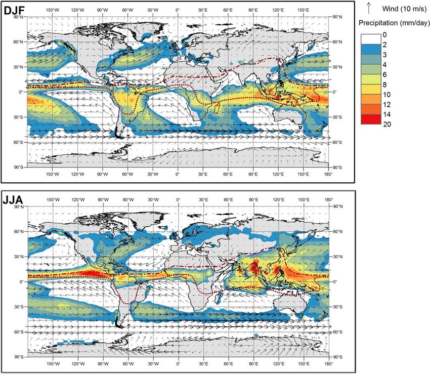
Monsoon circulation can result in air-mass mixing and high precipitation (McGregor and
Nieuwolt 1998; Zhang and Wang 2008), and in several monsoon regions the bands of
highest summer precipitation approximately follow the position of the ITCZ (Figure 7).
However, climate model simulations and reanalysis data indicate that not all areas
experiencing high precipitation are strongly influenced by air masses from the opposing
hemisphere. In particular, reanalysis data for the past 3 decades (Figure 7) shows that the
intrusion of NH air into the southeast trending South Pacific Convergence Zone (SPCZ) is
sharply truncated (but see Section 4.2). We therefore consider it more prudent to use wind
data and the seasonal ITCZ positions rather than precipitation to estimate the zonal
boundaries of the areas in which IntCal20, SHCal20 and a mixed curve are used.
We therefore recommend the use of (i) IntCal20 for areas north of the ITCZ in June–August
(dashed lines in Figure 7) which receive NH air masses all year round, (ii) SHCal20 for areas
south of ITCZ in December–February (dotted lines in Figure 7) which see SH air masses all
year round, and (iii) a mixed curve for areas between the two seasonal ITCZ positions shown in
Figure 7, which receive northern air masses in December–February and southern air masses in
June–August.
The degree of north-south air-mass mixing for the mixed curve is another issue. For vegetation,
which grows almost all year round, the degree of air-mass mixing should be 50%:50%
(northern:southern air masses). For seasonal vegetation, the degree of air-mass mixing
Downloaded from https://www.cambridge.org/core. IP address: 46.4.80.155, on 17 Dec 2021 at 23:18:57, subject to the Cambridge Core terms of use, available at
https://www.cambridge.org/core/terms. https://doi.org/10.1017/RDC.2020.59774 A G Hogg et al.
Figure 7 World map showing means of winds (1981–2010) and precipitation (1979–2018) at 925 hPa for two
different periods: December–February (top panel) and June–August (bottom panel). These data are derived from
the NCEP reanalysis wind (https://www.esrl.noaa.gov/psd/data/gridded/data.ncep.reanalysis.derived.pressure.html)
and the CMAP precipitation (Xie and Arkin 1997), respectively. Dotted and dashed lines represent the ITCZ
during December–February and June–August, respectively.
might be different than the above value. However, Hua and Barbetti (2007) estimated a 52 ± 13%
contribution of southern air masses to northern tropical and subtropical regions influenced by
monsoons during the boreal summer months, which was based on atmospheric and tree-ring 14C
data during the bomb-peak period. We thus recommend a simple approach with 50%:50% of
north-south air-mass mixing for the mixed curve, and age calibration using that curve can be
easily carried out using the “Mix_curve” command in OxCal program (Bronk Ramsey, 2009)
or selected as a curve option in CALIB 8.2 (Stuiver et al. 2020).
4.2 Past ITCZ variations
As the mean seasonal positions of the ITCZ and the strength of monsoon circulation change at
different timescales (inter-annual, decadal, centennial, etc.; e.g., Haug et al. 2001), the
boundaries of the mixed-curved areas in the past can be different from those shown in
Figure 7, which are based on the modern meteorological data. At least for the remote past,
Downloaded from https://www.cambridge.org/core. IP address: 46.4.80.155, on 17 Dec 2021 at 23:18:57, subject to the Cambridge Core terms of use, available at
https://www.cambridge.org/core/terms. https://doi.org/10.1017/RDC.2020.59SHCal20 Southern Hemisphere Calibration 775
the use of IntCal, SHCal or a mixed curve for a particular region in the tropics and subtropics
becomes less critical for many studies when the maximum 14C offsets of these curves, which are
the N-S offsets of 36 ± 27 14C yrs (based upon our estimates in Section 3.5) are negligible
compared to the ages of the events to be dated.
However, this may not be the case for researchers studying human expansion over short time
scales. For example, Goodwin et al. (2014) have reconstructed Pacific climate and in particular
wind field patterns associated with changing El Niño and La Niña events, over the last ~1000
yrs, using a general circulation climate model extensively calibrated with paleoclimate data.
Their model showed large variations on decadal and longer timescales in the mixing of NH
air into the South Pacific via the SPCZ, dependent on the state of the Pacific Decadal
Oscillation and the decadal-scale predominance of El Niño vs La Niña events, with
minimal mixing in some bi-decades and a mixed region extending as far as 30°S across
most of the Pacific in others.
It seems highly likely that similarly detailed wind field reconstructions in other areas will also
show significant variations in the past boundaries of the zone covered by the movement of the
ITCZ. Until new tree-ring 14C data sets are created from within the tropics and subtropics, only
approximations for the boundaries of the mixed region and the regional balance of northern
and southern air masses within it are possible, and researchers wishing to calibrate radiocarbon
data from these regions should be mindful of these limitations. Future research efforts should
focus on 14C measurement on tree rings from these areas in order to construct proper
calibration curves for these regions, and to gain a better understanding of regional 14C
offsets and their temporal variations.
5. HIGH SOUTHERN LATITUDES
De Pol-Holz et al. (2017) have suggested that an additional high latitude SH region should be
distinguished, as the region south of the peak intensity of the Southern Westerly Winds (~50°S)
is influenced by the release of old carbon from the Southern Ocean due to upwelling and air-sea
gas exchange. Turney et al. (2016) and Hogg et al. (2019) also found lower 14C levels from
Campbell Island (53°S) tree rings, supporting this finding. We have not implemented such
a feature in this version of SHCal, but researchers calibrating measurements from the
subantarctic SH should be aware of the likelihood that a small and likely time-varying
offset exists. As more calibration data from southern South America and subantarctic
islands in the Southern Ocean become available, we anticipate that a separate high latitude
Region 1 will likely be incorporated into future versions of SHCal.
ACKNOWLEDGMENTS
TJ Heaton is supported by a Leverhulme Trust Fellowship RF-2019-140\9, “Improving the
Measurement of Time Using Radiocarbon”. We would like to thank Stuart Hankin and
Jagoda Crawford for the preparation of Figure 7, and Duncan Christie and Ed Cook for
providing additional information on the tree ring dating of PAT02 (dataset 9-5) and
TAS01 (dataset 9.6) respectively.
SUPPLEMENTARY MATERIAL
To view supplementary material for this article, please visit https://doi.org/10.1017/RDC.2020.59
Downloaded from https://www.cambridge.org/core. IP address: 46.4.80.155, on 17 Dec 2021 at 23:18:57, subject to the Cambridge Core terms of use, available at
https://www.cambridge.org/core/terms. https://doi.org/10.1017/RDC.2020.59776 A G Hogg et al.
REFERENCES
Boswijk G, Fowler A, Palmer J, Fenwick P, Hogg A, Hogg A, Palmer J, Boswijk G, Turney C. 2011. High-
Lorrey A, Wunder J. 2014. The late Holocene precision radiocarbon measurements of tree-ring
kauri chronology: assessing the potential of a dated wood from New Zealand: 195 BC–AD
4500-yrs record for palaeoclimate reconstruc- 995. Radiocarbon 53(3):529–542.
tion. Quaternary Science Reviews 90:128–142. Hogg A, Turney C, Palmer J, Cook E, Buckley B.
Bronk Ramsey CB. 2009. Bayesian analysis of 2013a. Is there any evidence for regional 14C
radiocarbon dates. Radiocarbon 51:337–360. offsets in the Southern Hemisphere? Radiocarbon
Buck CE, Blackwell PG. 2004. Formal statistical 55(4):2029–2034.
models for estimating radiocarbon calibration Hogg AG, Hua Q, Blackwell PG, Niu M, Buck CE,
curves. Radiocarbon 46: 1093–1102. Guilderson TP, Heaton TJ, Palmer JG, Reimer PJ,
Büntgen U, Wacker L, Galván JD, Arnold S, Reimer RW, Turney CS. 2013b. SHCal13 Southern
Arseneault D, Baillie M, Beer J, Bernabei M, Hemisphere calibration, 0–50,000 years cal BP.
Bleicher N, Boswijk G, et al. 2018. Tree rings Radiocarbon 55(4):1889–1903.
reveal globally coherent signature of cosmogenic Hogg A, Turney C, Palmer J, Southon J, Kromer B,
radiocarbon events in 774 and 993 CE. Nature Bronk Ramsey C, Boswijk G, Fenwick P,
Communications 9:3605. doi: 10.1038/s41467- Noronha A, Staff R, Friedrich M. 2013c. The
018-06036-0. New Zealand kauri (Agathis australis) research
De Pol-Holz R, Santos GM, Ancapichun S, Southon J, project: a radiocarbon dating intercomparison
Collado S, Aravena JC, Christie D, Lara D, of Younger Dryas wood and implications for
Le Quesne C, Creasman PP, Reimer P. 2017. IntCal13. Radiocarbon 55(4):2035–2048.
Radiocarbon content in annual tree-rings from Hogg A, Southon J, Turney C, Palmer J, Ramsey CB,
western South America: The “Bomb” period Fenwick P, Boswijk G, Büntgen U, Friedrich M,
1950–2015 AD. 14th International AMS Helle G, Hughen K. 2016a. Decadally resolved
Conference, University of Ottawa, Canada, lateglacial radiocarbon evidence from New
August 14-18 2017 (abstr.) Zealand kauri. Radiocarbon 58(4):709–733.
Gelman A, Carlin JB, Stern HS, Rubin DB. 2013. Hogg A, Southon J, Turney C, Palmer J, Bronk
Bayesian data analysis. 3rd ed. Chapman and Hall. Ramsey C, Fenwick P, Boswijk G, Friedrich M,
Goodwin ID, Browning SA, Anderson AJ. 2014. Helle G, Hughen K, Jones R, et al. 2016b.
Climate windows for Polynesian voyaging to Punctuated shutdown of Atlantic Meridional
New Zealand and Easter Island. PNAS 111(41): Overturning Circulation during Greenland
14716–14721. doi: 10.1073/pnas.1408918111. Stadial 1. Nature Scientific Reports 6:25902. doi:
Güttler D, Adolphi F, Beer J, Bleicher N, Boswijk G, 10.1038/srep25902.
Christl M, Hogg A, Palmer J, Vockenhuber C, Hogg A, Gumbley W, Boswijk G, Petchey F,
Wacker L, Wunder J. 2015. Rapid increase Southon J, Anderson A, Roa T, Donaldson L.
in cosmogenic 14C in AD 775 measured in New 2017. The first accurate and precise calendar
Zealand kauri trees indicates short-lived increase dating of New Zealand Māori Pā, using Otāhau
in 14C production spanning both hemispheres. Pā as a case study. Journal of Archaeological
Earth and Planetary Science Letters 411:290–297. Science: Reports (12):124–133.
Haug GH, Hughen KA, Sigman DM, Peterson LC, Hogg A, Heaton T, Bronk Ramsey C, Boswijk G,
Röhl U. 2001. Southward migration of the Palmer J, Turney C, Southon J, Gumbley W.
Intertropical Convergence Zone through the 2019. The influence of calibration curve
Holocene. Science 293(5533):1304–1308. construction and composition on the accuracy
Heaton TJ, Blackwell PG, Buck CE. 2009. A and precision of radiocarbon wiggle-matching
Bayesian approach to the estimation of radio- of tree rings, illustrated by Southern Hemisphere
carbon calibration curves: The IntCal09 atmospheric data sets from AD 1500–1950.
methodology. Radiocarbon 51(4):1151–1164. Radiocarbon 61:1265–1291.
Heaton TJ, Blaauw M, Blackwell PG, Bronk Ramsey Hua Q, Barbetti M, Zoppi U, Fink D, Watanasak M,
CB, Reimer PJ, Scott EM. 2020. The IntCal20 Jacobsen GE. 2004a. Radiocarbon in tropical
approach to radiocarbon calibration curve tree rings during the Little Ice Age. Nuclear
construction: a new methodology using Bayesian Instruments and Methods in Physics Research B
splines and errors-in-variables. Radiocarbon 62. 223–224:489–494.
This issue. doi: 10.1017/RDC.2020.46. Hua Q, Barbetti M, Zoppi U. 2004b. Radiocarbon in
Hogg AG, McCormac FG, Higham TF, Reimer PJ, annual tree rings from Thailand during the
Baillie MG, Palmer JG. 2002. High-precision prebomb period, AD 1938–1954. Radiocarbon
radiocarbon measurements of contemporaneous 46:925–932.
tree-ring dated wood from the British Isles and Hua Q, Barbetti M. 2007. Influence of atmospheric
New Zealand: AD 1850–950. Radiocarbon circulation on regional 14CO2 differences. Journal
44(3):633–640. of Geophysical Research 112:D19102.
Downloaded from https://www.cambridge.org/core. IP address: 46.4.80.155, on 17 Dec 2021 at 23:18:57, subject to the Cambridge Core terms of use, available at
https://www.cambridge.org/core/terms. https://doi.org/10.1017/RDC.2020.59You can also read