Sensitivity of simulations of Zambian heavy rainfall events to the atmospheric boundary layer schemes
←
→
Page content transcription
If your browser does not render page correctly, please read the page content below
Sensitivity of simulations of Zambian
heavy rainfall events to the atmospheric
boundary layer schemes
Article

Published Version

Creative Commons: Attribution 4.0 (CC-BY)

Open Access

Bopape, M.-J. M., Waitolo, D., Plant, R. S. ORCID:
https://orcid.org/0000-0001-8808-0022, Phaduli, E., Nkonde,
E., Simfukwe, H., Mkandwire, S., Rakate, E. and Misha, R.
(2021) Sensitivity of simulations of Zambian heavy rainfall
events to the atmospheric boundary layer schemes. Climate, 9
(2). 38. ISSN 2225-1154 doi:
https://doi.org/10.3390/cli9020038 Available at
http://centaur.reading.ac.uk/95301/

It is advisable to refer to the publisher’s version if you intend to cite from the
work. See Guidance on citing .

To link to this article DOI: http://dx.doi.org/10.3390/cli9020038

Publisher: MDPI

All outputs in CentAUR are protected by Intellectual Property Rights law,
including copyright law. Copyright and IPR is retained by the creators or other
copyright holders. Terms and conditions for use of this material are defined in
the End User Agreement .

www.reading.ac.uk/centaur

CentAUR

Central Archive at the University of Reading
Reading’s research outputs online
climate
Article
Sensitivity of Simulations of Zambian Heavy Rainfall Events to
the Atmospheric Boundary Layer Schemes
Mary-Jane M. Bopape 1 , David Waitolo 2, * , Robert S. Plant 3 , Elelwani Phaduli 1 , Edson Nkonde 2 ,
Henry Simfukwe 4 , Stein Mkandawire 4 , Edward Rakate 5 and Robert Maisha 1

                                           1   South African Weather Service, Private Bag X097, Pretoria 0001, South Africa;
                                               Mary-Jane.Bopape@weathersa.co.za (M.-J.M.B.); Elelwani.Phaduli@weathersa.co.za (E.P.);
                                               Robert.Maisha@weathersa.co.za (R.M.)
                                           2   Zambia Meteorological Department, P.O. Box 50065, Lusaka, Zambia; edson.nkonde@mtc.gov.zm
                                           3   Department of Meteorology, University of Reading, Reading RG6 6ET, UK; r.s.plant@reading.ac.uk
                                           4   Zambia Research and Education Network, School of Education Building First Floor, University of Zambia,
                                               West Wing P.O. Box 32379, Lusaka, Zambia; henry.simfukwe@zamren.zm (H.S.);
                                               mkandaws@zamren.zm (S.M.)
                                           5   Centre for High Performance Computing, Council for Scientific and Industrial Research, P.O. Box 395,
                                               Pretoria 0001, South Africa; ERakate@csir.co.za
                                           *   Correspondence: david.waitolo@mtc.gov.zm

                                           Abstract: Weather forecasting relies on the use of numerical weather prediction (NWP) models,
                                           whose resolution is informed by the available computational resources. The models resolve large
                                           scale processes, while subgrid processes are parametrized. One of the processes that is parametrized
                                           is turbulence which is represented in planetary boundary layer (PBL) schemes. In this study, we
                                           evaluate the sensitivity of heavy rainfall events over Zambia to four different PBL schemes in the
                                 Weather Research and Forecasting (WRF) model using a parent domain with a 9 km grid length and

                                           a 3 km grid spacing child domain. The four PBL schemes are the Yonsei University (YSU), nonlocal
Citation: Bopape, M.-J.M.; Waitolo, D.;    first-order medium-range forecasting (MRF), University of Washington (UW) and Mellor–Yamada–
Plant, R.S.; Phaduli, E.; Nkonde, E.;
                                           Nakanishi–Niino (MYNN) schemes. Simulations were done for three case studies of extreme rainfall
Simfukwe, H.; Mkandawire, S.;
                                           on 17 December 2016, 21 January 2017 and 17 April 2019. The use of YSU produced the highest
Rakate, E.; Maisha, R. Sensitivity of
                                           rainfall peaks across all three cases; however, it produced performance statistics similar to UW that
Simulations of Zambian Heavy
                                           are higher than those of the two other schemes. These statistics are not maintained when adjusted for
Rainfall Events to the Atmospheric
Boundary Layer Schemes. Climate
                                           random hits, indicating that the extra events are mainly random rather than being skillfully placed.
2021, 9, 38. https://doi.org/              UW simulated the lowest PBL height, while MRF produced the highest PBL height, but this was not
10.3390/cli9020038                         matched by the temperature simulation. The YSU and MYNN PBL heights were intermediate at the
                                           time of the peak; however, MYNN is associated with a slower decay and higher PBL heights at night.
Received: 16 December 2020                 WRF underestimated the maximum temperature during all cases and for all PBL schemes, with a
Accepted: 4 January 2021                   larger bias in the MYNN scheme. We support further use of the YSU scheme, which is the scheme
Published: 23 February 2021                selected for the tropical suite in WRF. The different simulations were in some respects more similar
                                           to one another than to the available observations. Satellite rainfall estimates and the ERA5 reanalysis
Publisher’s Note: MDPI stays neu-
                                           showed different rainfall distributions, which indicates a need for more ground observations to assist
tral with regard to jurisdictional clai-
                                           with studies like this one.
ms in published maps and institutio-
nal affiliations.
                                           Keywords: flooding; weather forecasting; high performance computing; boundary layer scheme

Copyright: © 2021 by the authors. Li-
censee MDPI, Basel, Switzerland.           1. Introduction
This article is an open access article          During the period 1995 to 2015, floods accounted for 47% of all weather-related
distributed under the terms and con-
                                           disasters, affecting about 2.3 billion people [1]. Of the high impact events discussed in
ditions of the Creative Commons At-
                                           the State of the Climate in Africa 2019 report [2], flooding events were the most reported.
tribution (CC BY) license (https://
                                           Loss of life due to storms is higher in lower-income countries, which account for 89% of
creativecommons.org/licenses/by/
                                           the deaths, despite these countries experiencing just over a quarter of all the storms [1].
4.0/).

Climate 2021, 9, 38. https://doi.org/10.3390/cli9020038                                                      https://www.mdpi.com/journal/climate
Climate 2021, 9, 38 2 of 31
Adverse impacts of extreme weather and climate events on society can be reduced in the
presence of accurate and actionable early warnings, especially for rainfall [3].
In Zambia, the provision of weather and climate services is a mandate of the Zambia
Meteorological Department (ZMD) [4]. ZMD was established on 1st January 1967 as a
specialized agency with a core responsibility to provide meteorological services to aviation.
Due to increases in the severity and frequency of extreme weather events, ZMD is now
facing increasing demands for meteorological products and services. Sectors such as
agriculture, water, energy and health, along with the Disaster Management Unit, need
meteorological information for the purposes of planning, decision-making and policy
formulation for mitigation and adaptive strategies against extreme weather events and
climate change.
To provide weather forecasts, ZMD runs the Weather Research and Forecasting
(WRF) [5] numerical weather prediction (NWP) model, which has been running since
December 2019. The grid length used is 14 km. Forecasters also have access to Meteo
France ARPÉGE [6] (Action de Recherche Petite Echelle Grande Echelle) and the United
Kingdom Met Office (UKMO) Unified Model (UM) [7] outputs through a PUMA 2015
forecaster workstation. In addition forecasters also use output from the Global Fore-
cast System (GFS) [8] and the European Centre for Medium-Range Weather Forecast
(ECMWF) integrated forecasting system (IFS) [9] global products via the Internet. Other
platforms such as TAMSAT (Tropical Applications of Meteorology using SATellite data
and ground-based observations) [10], SWFDP (Severe Weather Forecasting Demonstration
Project) [11] and PUMA/MESA (Monitoring for Environment and Security in Africa) 2015
synergie (Eumetcast l (https://www.eumetsat.int/website/home/Data/DataDelivery/
EUMETCast/index.html) system) are used as well. There are 68 automatic weather stations
dotted around the country transmitting real time data every 15 min, of which 10 transmit
to the World Meteorological Office (WMO) website [12]. Venäläinen et al. [4] conducted a
situational analysis of ZMD and recommended a number of changes, including an increase
in the number of observing stations, a weather radar system and a forecast post-processing
system to assist the organization to produce early warnings.
Increases in available computational resources have resulted in an increase in res-
olution used by NWP models over the last few decades [13]. The ECMWF and UKMO
run global NWP models with grid spacings of 9 and 10 km, respectively. The two or-
ganizations announced large investments in their high performance computing (HPC)
systems of 80 million euro [14] and £1.2 billion [15] during early 2020. The African con-
tinent has largely lagged behind with developments in HPC; however, the situation has
started to improve. Through the Southern African Development Community (SADC)
Cyber-Infrastructure (CI) Framework, High Performance Computing systems have been
deployed in a number of countries within SADC, including Zambia [16].
The HPC system in Zambia is hosted by the University of Zambia at the Zambia
Research and Education Network (ZAMREN) HPC facility, and this is the system in use for
the current study. The availability of an HPC system in Zambia provides an opportunity
for ZMD to conduct NWP research to understand atmospheric processes, and to also
determine a suitable configuration for simulating weather and climate in Zambia [17].
Kanno et al. [18] did a 10 year climate simulation with WRF version 3.2 and found the
model overestimated rainfall on three sites in the southern province of Zambia. The
representations of subgrid processes such as clouds and turbulence are thought to be
responsible for much of the uncertainty in weather and climate simulations [19].
Turbulence plays an important role in the development, evolution and diurnal cycle
of the planetary boundary layer (PBL) and in the mixing of momentum, heat, moisture
and cloud water [20]. Turbulence is produced by a number of atmospheric processes,
including buoyant convection, shear forces and cloud-related radiative processes [21].
In most NWP models, turbulence is not resolved, but is parametrized using column-
based PBL schemes [19], within which the PBL height is considered as a key quantity [22].
Qian et al. [23] showed that the choices of PBL and surface layer schemes have largeClimate 2021, 9, 38 3 of 31
impacts on the simulation of surface moisture flux, convection initiation and precipitation
over the tropical ocean. There are two main forms of parametrization within PBL schemes:
local treatments influence only the model levels immediately adjacent to a given level, and
nonlocal treatments are designed to represent the impacts of large eddies such as those in
convective PBLs [19].
A number of studies have been conducted in different parts of the globe to assess the
performances of different PBL schemes. Jahn and Gallus [24] found the Yonsei University
(YSU) [25] and Mellor–Yamada–Nakanishi–Niino (MYNN) [26] PBL schemes to have
similar performances when simulating wind speed, but with a warm potential temperature
and dry specific humidity bias in YSU compared to MYNN when simulating the Great
Plains Low-Level jet. Bélair et al. [27] found a local turbulent kinetic energy (TKE)0based
scheme to underestimate the rapid evolution of the PBL in clear moderate and shear-driven
convective cases in Montreal. There was more sensitivity to a dry bias in the formulation
of the turbulent length scales than to the introduction of a nonlocal term. Cohen et al. [28]
compared two local, two non-local and one hybrid local–nonlocal scheme in simulations
of United States cold season severe thunderstorms, and concluded that the local schemes
produce overly weak vertical mixing and that nonlocal schemes overmix the boundary
layer. Comin et al. [29] found nonlocal schemes to perform better in Brazil than local
schemes when simulating an extreme rainfall event. When comparing a local, a hybrid
local–nonlocal and non-local schemes, Hu et al. [30] found the local scheme to produce
larger cold and moist biases than the other two over the South Central United States.
de Lange et al. [31] compared four PBL schemes in WRF over the Highveld of South
Africa for June and November 2016 and found the performance to not only be site-specific
but variable-specific also. They recommended the use of local schemes for winter; all
simulations were better in general compared to November. In this study we compare
the performances of four planetary boundary layer schemes in simulating three heavy
rainfall events over the southern parts of Zambia. An understanding of the performances
of different PBL schemes has implications for operational forecasting, and hence early
warnings because the best available scheme has to be established. The next section describes
the study area, followed by the simulation design and the data used in the study. The
rainfall events are described in Section 4, and simulation results are presented and discussed
in Section 5. A summary and conclusions are given in Section 6.
2. Study Area
Zambia is a landlocked country that occupies a near central location on the southern
African sub-continent between 8◦ and 18◦ S latitude, and 22◦ and 34◦ E longitude. The
Indian Ocean is the nearest sea, and is approximately 800 km to the east. Both the Indian
and Atlantic oceans are important sources of moisture for Zambia [32]. The wet years or
wet spells are dominated by low level westerlies, which oppose the mean easterly flow,
resulting in a low-level convergence of moisture over the country [32,33]. Zambia’s climate
is influenced by the equatorial low and the Inter-Tropical Convergence Zone (ITCZ) with
its southward and northward movements over Africa in different months of the year [34].
The rains brought by the ITCZ are characterized by thunderstorms, and are occasionally
severe, with much lightning [35] and sometimes hail.
Kanno et al. [18] found that the location of the ITCZ resulted in large intra-seasonal
variations in three summer seasons that they studied over southern Zambia (from 2007/2008
to 2009/2010). The El Niño Southern Oscillation (ENSO) has also been found to impact
the rainfall season of Zambia, with cool ENSO events being associated with increased
rainfall [36]. Hachigonta and Reason [33] found a stronger ENSO signal in the southern
parts of Zambia than in the north. The climate of the country is also modulated by altitude
(the topography is shown in Figure 1). The rainfall distribution is characterized by a down-
ward gradient from north to south, with annual amounts greater than 1200 mm reported in
the north-west and north east of the country, and the lowest amounts in the south-west [34].Climate 2021, 9, 38 4 of 31
The northern parts of Zambia receive most of their rainfall from November to March, with
a peak between December and January [36].
Many of the economic, cultural and social elements of the country are dominated by
the onset and end of the rainy season, and the amount of rain it brings [34]. More than
90% of the annual rainfall occurs in the rainy season, while 8% falls in October and April,
and 2% in September and May. Extreme events like droughts [37] and floods are frequent
occurrences in Zambia. They have caused crop damage and loss leading to food scarcity
and hunger, increases in diseases (malaria, dysentery, cholera, etc.) [38], destruction and
damage of infrastructure (houses, buildings, roads, bridges) [39], reduced charcoal business,
decline in fish catches and loss of life (humans and livestock). Thurlow and Diao [40]
indicated that climate variability reduced the gross domestic product of Zambia by about
4% and increased the number of people living below the poverty line by 2% over a ten
year period.
Figure 1. The outer domain of the 9 km grid length model and the 3 km grid length child domain (red box) with country
names and location of Lake Kariba indicated. The colors indicate topography in m.
3. Model, Data and Simulations
The Advanced Research WRF (ARW) model version 4.1.2 [5] was used in this study,
with four different boundary layer schemes as described below. WRF was chosen because
it is an open source community model, with many physics choices, and can be used for
operational forecasting without any associated license fee. The model can be used for
simulating processes with scales ranging from turbulent eddies to global systems. It is fully
compressible, with a nonhydrostatic option that allows convective-scale [41] simulationsClimate 2021, 9, 38 5 of 31
to be conducted. A wide range of choices can be made for the physical parametrizations.
Two physics suites are provided [42]: the CONUS suite, which is deemed suitable for the
Continental United States, and a tropical suite, which has been found to work well for the
tropical belt [43]. The tropical suite was selected for this study because of the location of
Zambia in the lower latitudes. It uses the rapid radiative transfer model (RRTM) for both
short and long wave radiation [44], the WRF Single Moment 6-class microphysical scheme
(WSM6) [45] and the new Tiedtke cumulus scheme [46–48].
3.1. Boundary Layer Schemes
In this study we tested the performances of four PBL schemes in simulating heavy
rainfall events over Zambia. We recognize that the 3 km grid length used in the study
approaches the gray-zone for the convective PBL when at its peak height (Section 5.3).
However, the aim of the study was to investigate different forms of column-based PBL
schemes in a real NWP context. Two of the schemes calculate a mixing length scale based
on turbulent kinetic energy (TKE), while the other two include a nonlocal contribution to
the turbulent fluxes to represent the mixing from large eddies in the daytime CBL [49].
Shallow cumulus convection is also considered in two of the schemes. The four schemes
used were:
• The Mellor–Yamada–Nakanishi–Niino (MYNN) PBL scheme [26]: this scheme is the
improved Mellor–Yamada scheme based on TKE.
• The Community Atmosphere Model (CAM) University of Washington (UW) Moist
Turbulence scheme [50]: this scheme is TKE based and also considers shallow
convection.
• The Medium Range Forecast (MRF) Model PBL scheme [51]: this scheme includes a
non-local term.
• The Yonsei University (YSU) PBL scheme [25]: this scheme includes a diagnostic
non-local term, and considers shallow convection, along with a top-down turbulence
contribution associated with cloud-top radiative cooling.
The schemes are further summarized in Table 1 for a quick reference on differences
amongst the four selected for this study.
Table 1. A summary of the schemes used.
Scheme Non-Local TKE-Based Shallow Convection
YSU Yes No Yes
UW No Yes Yes
MRF Yes No No
MYNN No Yes No
3.2. Simulation Design
A one-way nesting procedure was applied with WRF forced with the GFS data [8],
which provide time-dependent lateral boundary conditions (LBCs) for the outer domain,
updated every three hours of simulation time. The presentation of results focuses on WRF
simulations run from 16 April 2019 at 00:00 UTC until 18 April 2019 00:00 UTC. This event
was selected because it was associated with the highest rainfall amount recorded in 24 h in
2019 of 92.6 mm at Mount Makulu agromet weather station. Two further events were also
considered. A thirty hour simulation was done for 21 January 2017, on which 91 mm and
92.6 mm of rainfall were recorded within a 24 h period at the Mount Makulu agromet and
Lusaka city airport weather stations respectively. Additionally, selected was 17 December
2016, where 106 mm was reported within 24 h at Lusaka city airport weather station. The
location of Mount Makulu agromet station is indicated by a closed triangle, and the Lusaka
city station by a closed square in Figure 1, and they are at elevations of 1213 m and 1252 m,
respectively. These three cases represent the highest recorded rainfall amounts in the period
from 11 May 2016 (when the number of vertical levels in the GFS driving data increasedClimate 2021, 9, 38 6 of 31
from 27 to 32) to October 2020. The next highest amount is 73.2 mm which was recorded in
Livingstone on 7 February 2018; however, only cases with rainfall amounts greater than
90 mm in the southern parts of Zambia were considered in this study.
A nesting procedure was employed, with a 9 km grid length model domain nested
directly within GFS, and a child nest using a grid length of 3 km. The 9 km parent domain
spans 21.2◦ –34.82◦ E and 18.97◦ –6.88◦ S, while the 3 km domain covers 24.79◦ –29.34◦ E and
19.05◦ –14.69◦ S. Figure 1 shows the full 9 km domain, with the red rectangle showing the
smaller 3 km domain. The new Tiedtke scheme [46–48] for deep cumulus convection is
used for the 9 km model domain, but is switched off within the child domain, in line with
typical practice for convection-permitting resolutions (e.g., [41,52–54]).
3.3. Datasets
Quantitative precipitation estimates (QPE) from two satellite products were used to
study the spatial rainfall distribution. The first QPE used is TAMSAT developed at the
University of Reading [10,55]. TAMSAT provides daily rainfall estimates for all of Africa
on a 4 km grid. The second QPE is the 30 min interval Integrated Multi-satellitE Retrievals
for Global Precipitation Measurement (GPM) (IMERG) rainfall calibrated with ground
observations [56]. This dataset will be referred to as IMERG for the rest of the paper.
ERA5 is the latest climate reanalysis from ECMWF [57] and is used here to study other
variables, including temperature and winds. ERA5 combines vast amounts of historical
observations into global estimates using the IFS and data assimilation systems. Two ERA5
reanalysis products were used: the land surface variables with a grid spacing of 0.1◦ ,
referred to as ERA5_Land henceforth, and 0.25◦ data which shows the synoptic circulation
(ERA5 henceforth). The temporal interval provided by both IMERG and ERA5 makes
it possible for us to study the timing of rainfall, whereas TAMSAT is only available at
daily intervals.
Ground observations for maximum and minimum temperature, and twenty-four hour
rainfall from ZMD were also used to verify the model. The number of reporting stations
differs per event and per variable. For 17 December 2016, 17 stations were used for mini-
mum temperature, 15 for maximum temperature and 18 for rainfall. On 21 January 2017,
16 stations reported minimum temperature, 17 reported maximum temperature and 18
reported 24 h rainfall. For the last case of 17 April 2019, 13 stations reported both minimum
and maximum temperature, and 14 reported twenty-four hour rainfall.
3.4. Verification Scores
A number of performance measures were calculated for all three case studies using
the Developmental Testbed Centre (DTC) Model Evaluation Tools (MET) software version
8.1.2. Verification statistics are presented for rainfall simulations for the 9 km model, using
the observational IMERG data. The model output was regridded onto the IMERG grid
using the Grid Analysis and Display System (GrADS) regrid function. The Method for
Object-Based Diagnostic Evaluation (MODE) tool [58–60] within MET was used. MODE
was designed to avoid the "double penalty" problem associated with traditional verification
measures by using matched areas or object pairs to calculate the performance statistics.
Object-based verification statistics are especially useful for convective scale models which
usually struggle with capturing exact rainfall locations [52]. A number of performance
statistics are calculated based on the contingency Table 2 and these are listed below in a
similar way to Beusch et al. [61].
Table 2. Contingency table for calculating the skill scores.
Observations
Yes No
Yes hits (H) false alarms (F)
Forecast
No misses (M) correct rejects (R)Climate 2021, 9, 38 7 of 31
The Probability of detecting yes (PODY) indicates the proportion of correctly predicted
events from total observed events. PODY ranges between 0 and 1, with 1 being the perfect
score, and it is given by:
H
PODY = . (1)
H+M
The false alarm ratio (FAR) indicates the proportion of false alarms to all forecasts, it
ranges from 0 to 1, with 0 being a perfect score. It is defined as:
F
FAR = . (2)
F+H
The critical success index (CSI) indicates proportion of hits in all predicted and missed
events. It ranges between 0 and 1, with 1 being a perfect score and is given by:
H
CSI = . (3)
H+F+M
The Gilbert skill score (GSS) is the CSI adjusted to account for random chance, and
has a perfect score of 1:
H − Hr
GSS = , (4)
H + F + M − Hr
where Hr denotes the hit rate that would occur due to chance,
( H + M)( H + F )
Hr = . (5)
( H + M + F + R)
The Hanssen–Kuiper discriminant (HK) indicates the ability of the forecast to classify
events and non-events (0 indicates no skill and 1, a perfect score):
H F
HK = − . (6)
H+M F+R
The Hiedke skill score (HSS) gives the proportion of correct predictions after removing
predictions that are correct due to random chance. A perfect score is given by a value of 1,
while 0 indicates no skill, and it is defined by:
( H + R) − ( Hr + Rr )
HSS = (7)
( H + M + F + R) − ( Hr + Rr )
where Rr denotes the rejection rate due to chance,
( F + R)( M + R)
Rr = . (8)
( H + M + F + R)
Performance verification statistics were also calculated using ZMD maximum and min-
imum temperature observations for all the case studies, and PBL schemes. The mean error
(ME) and root mean square error (RMSE) were calculated using simulations interpolated
to the available stations using the following equations:
ME = F̄ − Ō (9)
r
1 n 2
RMSE = Σi=1 Fi − Oi (10)
N
where F represents the simulations, O the observations and N the total number of reporting
weather stations.Climate 2021, 9, 38 8 of 31
4. Event Descriptions
The ERA5 mean sea level pressure (MSLP) overlaid with 10 m winds for all three cases
is shown in Figure 2. For the April 2019 case, the plot is made both for 16 April (Figure 2c)
and 17 April (Figure 2d). The MSLP plots show that the Atlantic Ocean high (AOH) was
ridging over the eastern parts of the subcontinent during all the three cases. The system
is associated with an onshore flow over the eastern coastline of the subcontinent whose
northward extension differs amongst the events. The onshore winds transport moist air
from the Indian ocean over land. The pressure is highest in the April 2019 event, and
the onshore winds on 17 April extend across the whole eastern coastline. Areas of lower
pressure can be seen over Namibia that extend into Botswana and South Africa during the
17 December 2016 and the 21 January 2017 events.
Figure 2. ERA5 mean sea level pressure (colors, hPa) overlaid with 10 m wind arrows at 09h00 UTC on (a) 17 December 2016,
(b) 21 January 2017, (c) 16 and (d) 17 April 2019. A scale for the wind arrows is provided by the 10 ms−1 arrow below
the panels.
On 16 April 2019, the AOH was ridging along the southern parts of the continent
and there was not much onshore flow along the eastern coastal region. The heavy rainfall
was observed on 17 April, when strong onshore flow had developed from the Indian
ocean. Hachigonta and Reason [33] found wet spells over Zambia to be associated with
an Angolan low which transports moisture from the tropical south-east Atlantic Ocean
and with low level westerly anomalies. Libanda et al. [32] also found low level westerly
flow to contribute towards anomalous wet seasons in Zambia. However, these three
events demonstrate that the Indian ocean can also be an important moisture source for wetClimate 2021, 9, 38 9 of 31
spells in Zambia. The upper air synoptic conditions were also considered and nothing of
significant note was observed for these cases near or over Zambia.
WRF is nested within the GFS, which provides the interpolated initial conditions
and the lateral boundary conditions. To determine whether GFS captured the general
synoptic circulation of the three events, the MSLP and 10 m winds were also plotted for
GFS (Figure 3). GFS captured the ridging AOH for all three cases, and the higher pressures
of the April 2019 case. The GFS also captured the difference in wind patterns along the east
coast on 16 and 17 April, with clearer onshore flow on 17 April. The simulated pressure
over land, however, is somewhat lower in general compared to ERA5. The Angola low is
clearer in the GFS than in the ERA5, with the lowest pressure over land.
Figure 3. As in Figure 2 but for the GFS driving data.
A number of studies have compared the performance of GFS and the ECMWF IFS (on
which ERA5 is based) in simulating tropical convection (e.g., [62,63]). Both systems have
been found to perform well for short lead times, especially up to 24 h ahead. Beyond this
time, the IFS was found to outperform the GFS in general, while the precipitation from
both modelling systems was considered to be not useful beyond 4 days based on a number
of metrics. Although there are differences in pressure over land, we conclude that the GFS
was able to capture the major features responsible for moisture transport over Zambia.
This implies that WRF was forced with suitable synoptic fields. It should be noted that the
GFS data were selected for the study because the data is readily available and open, and is
used to force NWP models in operational mode.Climate 2021, 9, 38 10 of 31
The African continent is characterized by sparse observations which make it difficult to
evaluate the performance of models [2]. To allow for a comparison of the spatial distribution
of rainfall, several observation products are compared, because the ground observations
are too limited to provide a useful distribution of rainfall. In Figure 4 we show rainfall
over Zambia for the three cases from TAMSAT and IMERG which provide satellite rainfall
estimates calibrated with ground observations. TAMSAT has higher resolution with a
grid length of 4 km, while IMERG has a grid length of 0.1◦ . In general the pattern of the
area covered by rainfall is similar in the two products, for the three events. The spatial
distribution covers most of Zambia on 17 December 2016, but excludes most of the north
eastern part of the country on 21 January 2017. On 17 April 2019 the rainfall area is
smaller, with most of the rainfall occurring in the north western parts of Zambia. TAMSAT
rainfall does not exceed 40 mm anywhere over Zambia for the 17 December 2016 and
21 January 2017 case studies, although some larger rainfall amounts are reported by this
product for the 17 April 2019 event. A comparison of the largest amounts on 17 December
2016 and 21 January 2017 indicates that TAMSAT underestimated the observed rainfall
for these two events, given that over 90 mm was reported by at least one station in the
southern parts of Zambia as indicated in the station rainfall shown in Figures 5a and 6a.
Figure 4. IMERG (a,c,e) and TAMSAT (b,d,f) twenty-four hour rainfall (mm) on 17 December 2016 (a,b), on 21 January 2012
(c,d) and on 17 April 2019 (e,f).Climate 2021, 9, 38 11 of 31
Figure 5. Twenty-four hour rainfall (mm) on 17 December 2016 from (a) ZMD station data, (d) ERA5_Land, along with that
from WRF simulations with the (b) YSU, (c) UW, (e) MRF and (f) MYNN PBL schemes.
Figure 6. Twenty-four hour rainfall (mm) on 21 January 2017 from (a) ZMD station data and (d) ERA5_Land, along with that
from Weather Research and Forecasting (WRF) simulations with the (b) YSU, (c) UW, (e) MRF and (f) MYNN PBL schemes.Climate 2021, 9, 38 12 of 31
The ERA5_Land reanalysis data are shown in Figures 5d to 7d for the three cases in
their order of occurrence. The ERA5_Land pattern differences for the three case studies are
also aligned with those observed by IMERG and TAMSAT. The rainfall amounts, however,
are generally smaller compared to IMERG. In previous heavy rainfall studies with strong
synoptic forcing from an ex-tropical cyclone over Botswana [64] and a cut-off low [65]
over Namibia [66], TAMSAT was found to severely underestimate rainfall compared to
ERA5 and IMERG. Thorne et al. [67] found TAMSAT to perform well over plateau, but
to underestimate rainfall in mountainous regions. Syama et al. [68] found TAMSAT to
perform worse than other products in estimating winter rainfall over southern Africa but
to perform well with summer rainfall, and they concluded that TAMSAT is geared for
ITCZ-related convective rainfall. Beck et al. [69] found ERA5 to outperform IMERG over
complex topography, while IMERG performed better in regions dominated by convective
storms over the United States. In this study the ERA5 rainfall with a 0.25◦ grid length was
also analysed and found to be closely aligned to the ERA5_Land. Given the large amount
of rainfall recorded by ground observations we conclude that TAMSAT (for two cases),
ERA5 and ERA5_Land underestimated the rainfall in these extreme cases, and we therefore
use IMERG to calculate the verification statistics described in Section 3.4.
Figure 7. Twenty-four hour rainfall (mm) on 21 January 2017 from (a) ZMD station data and (d) ERA5_Land, along with
that from WRF simulations with the (b) YSU, (c) UW, (e) MRF and (f) MYNN PBL schemes.Climate 2021, 9, 38 13 of 31
5. Comparison of Simulations
5.1. Twenty-Four Rainfall Eyeball Comparisons
The current section focuses on a comparison of WRF twenty-four hour rainfall
amounts using different boundary layer schemes. Figure 5 shows the simulated rain-
fall with the four boundary layer schemes on 17 December 2016, alongside the station
rainfall and ERA5_Land product. IMERG indicates rainfall over most of the domain, with
the exception of the extreme southern parts of the domain, with some areas exceeding
60 mm over the central parts (Figure 4a). Rainfall of over 60 mm is simulated in parts
of the inner 3 km domain. The ERA5_Land amounts are mainly lower, with an area of
higher rainfall along Lake Kariba (Figure 5d). All WRF configurations captured the gen-
eral rainfall pattern, but the larger rainfall amounts were not captured outside the 3 km
domain. The different simulations appear more similar to one another than they are to
IMERG and ERA5_Land. In a recent comparison of different microphysical schemes in
WRF, Molongwane et al. [64] also found the simulations to look more similar to one another
than to observations. YSU and UW simulated rainfall aligned parallel with the southern
border of Zambia and hence Lake Kariba, as also found in IMERG. These two schemes
include a component that represents the impact of shallow convection on mixing. The
alignment is less clear with MRF and MYNN.
Figure 6 is the same as Figure 5, but for 21 January 2017. The rainfall spatial coverage
is smaller than for 17 December 2016, and IMERG again (Figure 4c) indicates areas with
rainfall amounts exceeding 70 mm. Most of the north eastern part of the inner domain
has rainfall amounts exceeding 40 mm. This is not found in the ERA5_Land; however,
and we note that this cannot be attributed to resolution differences as the two datasets
are of similar resolution. The different WRF configurations did not capture the regions
with higher rainfall outside the 3 km domain, and they all produced a rainfall gap on the
northern boundary of the inner domain. Recalling the northerly flow across this boundary
(Figures 2b and 3b), the gap is likely a spin-up effect caused by adjustment from the
9 km configuration with parametrized convection to the 3 km convection-permitting
configuration. YSU, UW and MRF simulated the most rainfall in the north-western part of
the inner domain, whereas MYNN simulated a smaller area of higher rainfall further to
the south.
The total rainfall for 17 April 2019 is shown in Figure 7. TAMSAT estimated higher
rainfall amounts for this case with the largest rainfall estimates to the north-west of inner
domain (Figure 4f), while IMERG (Figure 4) presented larger amounts to the east of the
9 km domain. The ERA5_Land product (Figure 7d) indicated a continuous area of rainfall
over the whole northern portion of the inner domain. It also indicated slightly more
rainfall coverage to the north and north west of the inner domain (in agreement with
TAMSAT), although the ERA5_Land rainfall amounts are lower than TAMSAT. There is
a very clear qualitative difference in the WRF simulated rainfall between the 3 km and
9 km model domains. This difference reflects the different treatments of deep convection.
In particular, various small areas are simulated within the 3 km domain where rainfall
exceeds 50 mm. Similarly to other cases, there is a closer match between the different model
configurations than there is to the observations or between the different observations. YSU
and MRF produced the highest amount of rainfall in the north-west of the inner domain,
and both these schemes are non-local. The UW scheme is associated with the smallest peak
intensities, although it does produce some values greater than 50 mm, somewhat scattered
across the inner domain. It may be noted that YSU is the selected scheme for the tropical
suite [42].
5.2. Hourly Rainfall Eyeball Comparisons
In order to understand how the PBL schemes interact with the simulated convection,
the current and next two subsections present a closer investigation of the 17 April 2019 case,
the simulation for which starts on 16 April 2019. The area maximum hourly rainfall within
the 3 km inner domain is shown for the different WRF configurations in Figure 8a, withClimate 2021, 9, 38 14 of 31
corresponding results from IMERG and ERA5. As already discussed, ERA5 underestimated
the rainfall in this event, and this is apparent also in the hourly maximum plot. IMERG
estimated heavy rainfall outside the area of the inner domain and it produced lower
maximum values within that area. All of the WRF configurations simulated large maxima
on 17 April compared to the previous day. The simulated maxima are quite similar for the
first 9 h of the runs, but diverge later. The two non-local schemes (i.e., YSU and MRF) are
associated with the largest hourly rainfall peaks, although these were not simulated at the
same time. The MRF peak occurred at 1000 UTC on 17 April, and beyond that time MRF
typically simulated lower maxima than the other schemes.
Figure 8. Timeseries for the 3 km model domain of the simulated (a) maximum hourly rainfall,
(b) minimum temperature and (c) maximum 10 m wind speed from 00 UTC on 16 April to 00 UTC
on 18 April 2019. Results are shown using the YSU (blue), UW (gray), MRF (purple) and MYNN
(green) PBL schemes. Shown as well are results from the 0.25◦ (red) and 0.1◦ (orange) ERA5 products
and rainfall estimates from GPM (black).
The circulation patterns in Figure 2 showed moisture transport over land from the
Indian ocean on 17 April due to a ridging high pressure system. Figure 8a indicates that the
various WRF simulations captured the difference in the moisture source between 16 and
17 April. The WRF configurations are associated with higher resolution than both ERA5
datasets and IMERG, and this capacity to simulate the moisture–terrain interactions may
have been been a factor in producing the larger rainfall maxima over Zambia.
Figure 8b shows simulated minimum temperatures, while Figure 8c shows maximum
10 m wind speeds. These results are indicative of the influence of convective rainfall on the
formation and spreading of cold pools. The ERA5 minimum temperatures are higher than
in the WRF simulations over most of the period, especially in the first and last twelve hours.
The two ERA5 configurations are generally similar despite their different resolutions. The
ERA5 maximum wind speed is consistently lower than in WRF, with very little difference
between the 0.25◦ and 0.1◦ data. These points are consistent with an interpretation that theClimate 2021, 9, 38 15 of 31
weaker maximum rainfall in the domain in ERA5 is associated with weaker surface cold
pools. The same relationships have previously been found in idealized studies (e.g., [70]).
Further support for the idea is that the YSU configuration simulated the largest maximum
rainfall on 16 April, and this was matched by the lowest minimum temperature and the
largest maximum wind speed of the WRF simulations. Likewise, the peak rainfall from the
MRF configuration on 17 April is also associated with the lowest minimum temperature
and slightly higher wind speeds.
The area maximum rainfall, minimum temperature and maximum wind over the 3 km
domain were also studied for the 17 December 2016 and 21 January 2017 cases. The results
are consistent with the main findings from the 17 April 2019 case, with the maximum
rainfall from WRF far exceeding the IMERG and ERA5 maxima. YSU simulated the largest
rainfall peaks for 17 December 2016. The ERA5 and ERA5_Land area minimum tempera-
tures were higher than in all WRF simulations expect at 05h00 UTC, where ERA5_Land
is lower. MYNN and MRF simulated the highest area maximum wind peak, followed by
YSU whose peak occurred later. The ERA5 and ERA5_Land wind peaks are mostly similar,
and much weaker than the values in the WRF simulations. For the 21 January 2017 case,
YSU simulated the largest rainfall and strongest area maximum wind speed peak, followed
by MYNN. The ERA5 and ERA5_Land comparison to WRF simulations is consistent across
all three case studies, with ERA5 being associated with higher area minimum temperatures
and the lower area maximum wind speeds.
The area hourly average rainfall, temperature and wind speed for the 17 April 2019
case are shown in Figure 9. The average rainfall from the IMERG satellite estimate and
ERA5 reanalysis is greater than all the WRF simulations on 16 April. The situation is
different on 17 April where WRF simulated more rainfall than IMERG and ERA5. ERA5
indicates a shorter-lived event within the 3 km domain, which peaks about four hours
earlier than in IMERG. The different WRF configurations also produced a peak earlier than
IMERG, with timing that is more similar to the ERA5 reanalysis; however, the simulated
event is longer lived compared to ERA5. The start of the rainfall on 17 April is well matched
between the YSU and UW simulations. Both these schemes take shallow convection into
account. The simulations diverge beyond 1300 UTC, with YSU producing the most area
averaged rainfall of all the schemes. The MYNN and MRF simulations also captured the
event, although the peak was delayed by around an hour with MYNN compared to the
other schemes.
The area hourly average rainfall is also shown for the two other case studies in
Figure 10. The ERA5 and IMERG rainfall is higher than for all of the WRF simulations at
the beginning of the simulation period, which should be considered as a spin up period.
Champion and Hodges [71] found that model spin up for dynamical downscaling with
the Unified Model is between 6 and 12 h. Unlike the 17 April 2019 case, the IMERG area
average rainfall estimate in the 3km domain is generally higher than that in the WRF
simulations for the 17 December 2016 and 21 January 2017 cases. The rainfall in these two
cases is relatively long lived, persisting throughout the study period in both the satellite
estimates and WRF simulations.
The general findings from the average temperature and wind results are similar
across the three cases, and so these will be shown only for the 17 April 2019 case study
(Figure 9b,c). Relatively small differences are apparent in the WRF simulated average 2 m
temperatures, with MYNN being slightly cooler than the others and YSU being slightly
warmer during the peak on 17 April. The temperature peak occurs about two hours before
the rainfall peak. The rainfall peak occurs at 14h00 in the 17 December case with the
average temperature peaking between 12h00 and 13h00 UTC. The rainfall peak in the
21 January 2017 is observed at night, as shown in IMERG.
The ERA5 and ERA5_Land average wind speeds were markedly lower than in the
WRF simulations during much of the period. The YSU scheme simulated slightly stronger
winds, and the MYNN scheme slightly weaker winds amongst the WRF configurations.
These points were consistent across all three case studies.Climate 2021, 9, 38 16 of 31
Figure 9. As in Figure 8 but for hourly averages rather than extreme values.
Figure 10. Area average hourly rainfall for the (a) 17 December 2016 and (b) 21 January 2017
case studies.Climate 2021, 9, 38 17 of 31
In order to examine the spatial pattern of individual simulated thunderstorms, the
WRF simulated rainfall between 1100 to 1200 UTC on 17 April 2019 is shown in Figure 11.
The WRF model produced many separated rainfall objects, in contrast with the smoother,
larger and weaker areas found in the lower resolution observational estimate and reanal-
ysis product. The individual objects can produce large localized peaks, as confirmed by
Figure 8, which showed that some objects are associated with rainfall close to or exceeding
100 mm within one hour, while the area average rainfall is less than 2 mm for all config-
urations (Figure 9). The convection occurs through the interplay of surface heating and
topography, and local influences such as from previous convection, and the large-scale
moisture transport from the Indian ocean caused by the ridging high pressure system. The
location of the rainfall differs between ERA5 and IMERG, although both have the same
grid length of 0.1◦ .
The WRF configurations using YSU and UW, which both consider shallow convection
within the PBL scheme, simulated a line of thunderstorms at this time, which is aligned
with topography north of Lake Kariba. These two simulations also generated numerous
scattered objects with very light rainfall. The simulated structures using the MRF and
MYNN schemes are broadly aligned north-west to south-east and east to west respectively.
These configurations also produce broader areas with little or no rainfall.
Figure 11. Rainfall (mm) simulated within the 3 km model domain between 1100 and 1200 UTC on 17 April 2019 in WRF
runs using the (b) YSU, (c) UW, (e) MRF and (f) MYNN PBL schemes. The corresponding results from IMERG and from
ERA5_Land are shown in (a,d) respectively.Climate 2021, 9, 38 18 of 31
5.3. The Planetary Boundary Layer Height
The PBL height marks the transition from the boundary layer to the free atmosphere.
It is associated with a diurnal cycle [72], and its value is influenced by the turbulence
representation used. For example, in large-eddy simulations its value, and the bound-
ary layer temperature profile, were found to differ between the Smagorinky and the
dynamic Smagorinsky model, during both the morning transition [73] and CBL equilib-
rium stage [74]. The evolution of the PBL height as simulated by different configurations
of WRF is shown for the 17 April 2019 case in Figure 12a. The diurnal cycle is clear, with
a lower PBL height at night and early morning. The PBL height increases as the surface
warms after sun-rise, reaching an average PBL height of greater than 1000 m with all WRF
configurations. The most notable differences among the different schemes are that the area
averaged PBL height is greatest using MRF and smallest using UW, while the decay in the
early evening is delayed and is slower using the MYNN scheme.
The area minimum for each hour is shown in Figure 12b, and MYNN simulated
a markedly higher minimum during all the simulated hours. It also has a higher PBL
maximum (Figure 12c) between around 1500 to 0600 UTC, and a slower decay, which
is consistent with the evolution of the area average. MRF usually had the highest area
maximum at other times.
Figure 12. Timeseries for the 3 km model domain of the simulated (a) average, (b) minimum and (c) maximum PBL height
from 00 UTC on 16 April to 00 UTC on 18 April 2019. Results are shown using the YSU (blue), UW (gray), MRF (purple)
and MYNN (green) PBL schemes.Climate 2021, 9, 38 19 of 31
The area average PBL height is shown for the two other case studies in Figure 13. The
evolution of the PBL is similar across the three case studies, with MYNN being associated
with a higher PBL height at night and MRF having a higher PBL height between 06h00 and
15h00 UTC. The peak in PBL height is almost the same for MYNN and YSU, with a more
gradual decay for MYNN. UW consistently simulated the lowest daytime PBL height.
Figure 13. Timeseries for the 3 km model domain of the simulated average PBL height from (a) 00 UTC on 17 December to
06 UTC on 18 April 2016 and (b) 00 UTC on 21 January to 06 UTC on 22 Janaury 2017. Results are shown using the YSU
(blue), UW (gray), MRF (purple) and MYNN (green) PBL schemes.
To gain some understanding of the spatial structure of the PBL heights, and how it
relates to the rainfall distribution, we consider maps of the PBL height at 12h00 UTC on
17 April 2019 in Figure 14. These may be compared with the rainfall maps from Figure 11.
It is immediately clear that the areas with low PBL heights occur predominantly at and
around the areas of simulated rainfall. At this time Figure 12a showed that MYNN and
MRF have the same BL height which is higher than with YSU and higher again than with
UW. The low average height from UW is understandable from the spatial distribution
(Figure 14b) as arising from the large area of PBL heights with values less than 600 m. In
contrast, MYNN is associated with a relatively small area of PBL heights less than 600 m
(Figure 14d), matching the smaller area of rainfall in the preceeding hour (Figure 11f). The
MRF simulation has a larger area of low PBL heights than MYNN (Figure 14c), but the
same average is obtained because there are higher values in the south-west of the domain.Climate 2021, 9, 38 20 of 31
The line of convective storms that is simulated by YSU (Figure 11b) in alignment with the
topography can also be seen to have influenced the simulated PBL heights (Figure 14a).
Figure 14. The PBL height at 12h00 UTC on 17 April 2019 in WRF simulations using the (a) YSU, (b) UW, (c) MRF and (d)
MYNN PBL schemes.
All of the WRF configurations have some rainfall within the 3 km domain throughout
17 April 2019 (Figure 8) but the main period of intense simulated rainfall starts at around
10h00 UTC (Figure 9). In Figure 15 we show maps of the PBL height before that period,
at 09h00 UTC. All of the WRF simulations produce low values of less than 600 m around
Lake Kariba. The YSU (Figure 15a) and UW (Figure 15b) schemes have few locations with
low PBL heights otherwise. The MRF scheme produced small values over a larger area that
includes the lake (Figure 15c). This area is associated with the large peak in the maximum
rainfall around the same time, as shown in Figure 8. However, MRF again simulated high
values of PBL height over the south western part of the domain, leading it to have the
largest area average PBL height at this time (Figure 12a). The lowest area average height
occurred for the UW simulation, which has considerably larger areas with low PBL heights
(Figure 15b).Climate 2021, 9, 38 21 of 31
Figure 15. As in Figure 14 but for 09h00 UTC on 17 April 2019.
5.4. Near-Surface Temperatures
The analysis so far has demonstrated close connections between the spatial patterns of
rainfall and associated low PBL heights. A plausible explanation for this connection would
be the formation of cold pools by the convective storms, and their subsequent spreading as
density currents over the surface. The layer of cold air at the surface would be expected to
lead to a diagnosis of low PBL height. To test this idea, we have plotted spatial maps of 2 m
temperature at 12h00 UTC in Figure 16 for comparison with the rainfall (Figure 11) and
PBL heights (Figure 14). We also plot the temperature at 09h00 UTC in Figure 17. Indeed,
there is a close correspondence between these spatial patterns for all of the schemes tested.
The temperatures simulated by UW at 12h00 UTC (Figure 16a) are lower compared
to other configurations over most of the northern part of the domain. This result is con-
sistent with the lower PBL heights which were found in this configuration (Figure 14a),
and with the convection elements distributed over much of this area (Figure 11a). The
MYNN simulation is also found to be generally cooler, compared to MRF and YSU in this
same area (Figure 16d). Over the south western parts of the domain, MYNN is also some-
what cooler than the other configurations. The north-west to south-east aligned rainfall
(Figure 11d) and PBL height pattern (Figure 14d) is associated with cooler temperatures
in the MYNN simulation. MYNN does not simulate temperatures higher than 34 ◦ C,
which were produced by all other configurations along the eastern border of the 3 kmClimate 2021, 9, 38 22 of 31
domain. Interestingly MRF does not appear to be much warmer in the south western part
of the domain (Figure 16c) where high PBL heights were diagnosed by this PBL scheme
(Figure 14c).
Figure 16. The temperature at 12h00 UTC on 17 April 2019 in WRF simulations using the (a) YSU, (b) UW, (c) MRF and
(d) MYNN PBL schemes.
At 09h00 UTC, UW was found to be associated with lower PBL heights (Figure 12b) but
its simulated temperatures are not generally lower compared to other schemes (Figure 15b).
Rather, the MYNN scheme simulated lower temperatures in general (Figure 15b). Thus,
there is a less direct relationship between PBL heights and surface temperatures at this
time, in the absence of significant rainfall and cold pool formation. We note also that YSU
simulated higher temperatures in general compared to MRF (Figure 16a,c), even though
MRF produced higher BL heights (Figure 14a,c). However, the region that was associated
with lower PBL heights in the MRF simulation at 09h00 UTC, which was related to rainfall
above, was found to be associated with lower temperatures.Climate 2021, 9, 38 23 of 31
Figure 17. As in Figure 14 but for 09h00 UTC on 17 April 2019.
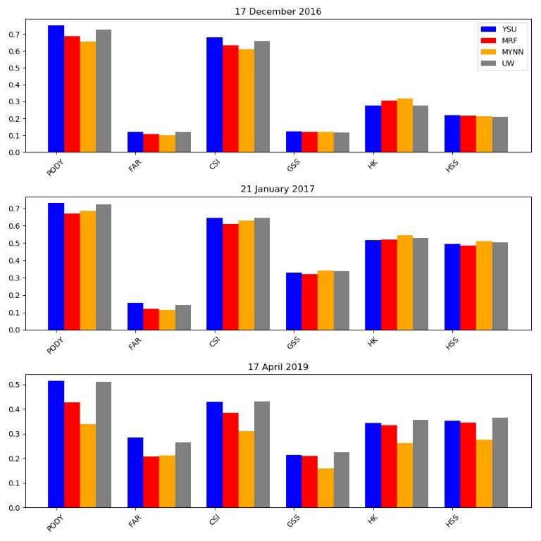
5.5. Verification Statistics
In this section, the performance statistics are discussed for simulated rainfall using
the four PBL schemes compared with IMERG. IMERG produced larger rainfall amounts
compared to the ERA5_Land and TAMSAT products, which underestimated rainfall com-
pared to the available ground station data for two of the three cases. The statistics are
summarized in Figure 18 and were calculated with the MODE tool in MET, as described in
Section 3.4.
The PODY is generally higher for YSU and UW, and MYNN produced the lowest
scores for the 17 December 2016 and 17 April 2019 case studies. The CSI and PODY statistics
show similar relative performances of the different PBL schemes. However, the FAR is also
higher for YSU and UW, with MYNN being associated with the lowest FAR in general.
The models’ performances on 17 December 2016 and 21 January 2017 are generally similar;
worse performances occurred for the 17 April case (note the change of scale in Figure 18c).
Differences in scores between the different PBL schemes are more readily apparent for the
17 April 2019 case.Climate 2021, 9, 38 24 of 31
Figure 18. Contingency table statistics calculated using MODE Tools for (a) 17 December 2016, (b) 21 January 2017 and
(c) 17 April 2019. The various quantities calculated are described in Section 3.4. Results are shown using the YSU (blue),
UW (gray), MRF (red) and MYNN (yellow) PBL schemes.
The GSS is lower than the CSI, and the YSU and UW schemes do not stand out relative
to the others for this metric, in contrast to PODY and CSI. A similar remark holds for
the HSS, where the MRF and MYNN are found to be slightly better in some instances,
compared to YSU or UW. This suggests that the higher PODY, CSI and FAR scores of UW
and YSU occur partly through random chance, because they tend to produce more rainfall
“events” (as in Figure 11 for example). Nonetheless, the MYNN GSS and HSS are clearly
lower than those of other schemes for the 17 April 2019 case study. The HK scores also
show some similar results across schemes, with YSU and UW performing at the same level
or slightly worse than MRF and MYNN on 17 December 2016 and 21 January 2017. For the
17 April 2019 case study, MYNN again stands out with a lower HK score.
ZMD minimum and maximum temperature observations were also used to test the
performance of different PBL schemes. The number of stations used differed per case,
ranging from 13 to 18 distributed across Zambia. The observed maximum temperatures
for all three cases are shown in Figure 19 to show the distribution of the available stations.
Not all stations are available for all the events—the April 2019 event being associated withClimate 2021, 9, 38 25 of 31
fewer stations. The corresponding simulated maximum temperature obtained from three-
hourly data for the YSU PBL scheme are also shown for eye ball verification. The results
suggest that the model generally underestimated the maximum temperature. The model
data were interpolated to the available stations for each case with a bilinear interpolation
method, using the nearest four grid points. The interpolated data were then used with the
corresponding observations to generate the ME and RMSE shown in Table 3 for all PBL
schemes, and the three case studies.
Figure 19. Observed station maximum temperatures on (a) 17 December 2016, (b) 21 January 2017 and (c) 17 April 2019,
and WRF simulated maximum temperature using YSU on (d) 17 December 2016, (e) 21 January 2017 and (f) 17 April 2019
based on three hourly output.
WRF underestimated the maximum temperature for all the case studies (Table 3).
MYNN is associated with the largest bias of all the PBL schemes, while the ranking for the
other schemes differs per case study. YSU has the lowest bias for the 17 December 2016 case,
MRF for 21 January 2017, and UW for 17 April 2019. The same result was found for the
RMSE, with MYNN being associated with the largest RMSE. For minimum temperature,
WRF simulated a slight warm bias for the 17 December 2016 case and 17 April 2019 case
studies, and a cool bias for MRF and MYNN for 21 Janaury 2017. MRF is associated with
the lowest RMSE for all the cases, when compared to YSU and UW, while MYNN has the
lowest of all for the 17 December 2016 case study.Climate 2021, 9, 38 26 of 31
Table 3. The mean error and root mean square error for the three case studies with four PBL schemes.
17 December 2016
YSU MRF MYNN UW
Bias −1.32012749 −1.38775444 −2.77817154 −1.38088036
Tmax
RMSE 0.486743391 0.493839473 0.977323115 0.588211000
Bias 1.46163368 1.44644737 1.04733276 1.35207367
Tmin
RMSE 0.352237523 0.259509355 0.141910866 0.322271198
21 January 2017
YSU MRF MYNN UW
Bias −2.41129112 −2.37238693 −3.80073738 −2.59328842
Tmax
RMSE 1.05125797 0.493839473 1.18280017 1.01926601
Bias 0.257066727 −0.03591537 −0.09047127 0.197696686
Tmin
RMSE 0.765877962 0.259509355 0.620617151 0.802365541
17 April 2019
YSU MRF MYNN UW
Bias −2.97936249 −2.92316628 −4.44790268 −2.87375450
Tmax
RMSE 1.00955522 1.01955235 1.48482561 0.488890052
Bias 0.302921295 0.432020187 0.01034927 0.177062988
Tmin
RMSE 0.603425622 0.444622010 0.662797749 0.645322680
6. Summary and Conclusions
Sensitivity tests of three heavy rainfall events that took place over Zambia with
different PBL schemes were conducted using the WRF model. The events were associated
with over 90 mm of rainfall in a 24 hour period for at least one ground station in the
southern part of Zambia. During all three events there was a ridging Atlantic Ocean high,
resulting in an onshore flow that transported moist air from the Indian ocean onto the
subcontinent. The GFS captured the synoptic conditions, with higher pressure associated
with the 17 April 2019 event. The pressure over land, however, was generally found to
be lower than in the ERA5 reanalysis. Uplift occurred due to surface heating and terrain,
resulting in isolated convection cells over the area of interest. The role of surface heating is
indicated by the lag of about 2 to 4 h between the peak in temperatures and the peak in
area average rainfall. Kanno et al. [18] also found a strong diurnal cycle in the rainfall of
Zambia, indicating strong afternoon convection, and large spatial differences in sites that
they studied due to differences in topography.
IMERG and TAMSAT satellite rainfall estimates, and ERA5 and ERA5_Land reanalysis
data, were used to study the spatial distribution of the rainfall during the three events.
IMERG produced rainfall amounts larger than 75 mm in parts of Zambia for all three
events, while TAMSAT rainfall was less than 40 mm for two of the events, with higher
amounts for the 17 April 2019 event. The ERA5 and ERA5_Land rainfall totals were also
mostly less than 40 mm over Zambia. It may be noted that the ERA5_Land has a similar
spatial resolution to IMERG. Given that the three events were selected because at least one
ground observation reported over 90 mm of rainfall, we conclude that IMERG provides the
best estimate of extreme rainfall. The QPE from TAMSAT for the 17 December 2016 and 21
January 2017 case studies is consistent with other recent studies in the region, in the sense
that values were severely underestimated in simulating heavy rainfall associated with
an ex-tropical cyclone [64] and a cut-off low system [66]. It may be noted that the ZMD
station rainfall was used to calibrate the TAMSAT QPE [10,55]. The location of maximum
rainfall differed across the different observational estimates, with none of them capturing
the largest values of rainfall found in the station observations.You can also read