SDOD: Real-time Segmenting and Detecting 3D Object by Depth
←
→
Page content transcription
If your browser does not render page correctly, please read the page content below
SDOD: Real-time Segmenting and Detecting 3D
                                                      Object by Depth

                                          Shengjie Li1 , Caiyi Xu1 , Jianping Xing1 , Yafei Ning1 , and YongHong Chen2
                                                      1
                                                        School of Microelectronics, Shandong University, Jinan, China
                                             2
                                                 City Public Passenger Transport Management Service Center of Jinan, China
arXiv:2001.09425v3 [cs.CV] 24 Oct 2020

                                                      lishengjie199012@126.com, cyxu@mail.sdu.edu.cn, {xingjp,
                                                             ningyafei}@sdu.edu.cn, chenyhjn@foxmail.com

                                                  Abstract. Most existing instance segmentation methods only focus on
                                                  improving performance and are not suitable for real-time scenes such as
                                                  autonomous driving. This paper proposes a real-time framework that seg-
                                                  menting and detecting 3D objects by depth. The framework is composed
                                                  of two parallel branches: one for instance segmentation and another for
                                                  object detection. We discretize the objects’ depth into depth categories
                                                  and transform the instance segmentation task into a pixel-level classifi-
                                                  cation task. The Mask branch predicts pixel-level depth categories, and
                                                  the 3D branch indicates instance-level depth categories. We produce an
                                                  instance mask by assigning pixels which have the same depth categories
                                                  to each instance. In addition, to solve the imbalance between mask labels
                                                  and 3D labels in the KITTI dataset, we introduce a coarse mask gen-
                                                  erated by the auto-annotation model to increase samples. Experiments
                                                  on the challenging KITTI dataset show that our approach outperforms
                                                  LklNet about 1.8 times on the speed of segmentation and 3D detection.

                                                  Keywords: Real-time Instance Segmentation, 3D Object Detection, Depth
                                                  Estimation

                                         1       Introduction

                                         With the development of automated driving technology, real-time instance seg-
                                         mentation and 3D object detection of RGB images play an increasingly impor-
                                         tant role. Instance segmentation combines object detection and semantic seg-
                                         mentation, help autonomous vehicles perceive complex surroundings. State-of-
                                         the-art approaches to instance segmentation like Mask R-CNN [10] and Fully
                                         Convolutional Instance-aware Semantic Segmentation (FCIS) [16] are only fo-
                                         cused on 2D objects and are still show poor performance in 3D scenes such
                                         as inaccurate semantic masks or error labels. Therefore, it is not enough to be
                                         used in autonomous driving. For more accurate 3D locations and shorter infer-
                                         ence time, some latest 3D object detection frameworks speed up by splitting
                                         3D tasks into multiple 2D related subtasks, like MonoGRNet [23] proposes a
                                         network composed of four task-specific subnetworks, responsible for 2D object
                                         detection, instance depth estimation, 3D localization and local corner regression.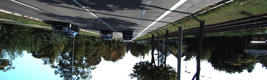
2       Li, S. et al.

In this paper, we focus on the real-time task fusion of instance segmentation and
3D object detection. Different from 3D instance segmentation based on the point
cloud, We propose a framework whose 3d branches and mask branches are par-
allel and proposal-free; when we input an image, it can output 3D location, 3D
bounding box and instance mask by depth in real-time, as shown in Fig. 1.

                                    Car   Car
                            Car

          (a)                     (b)                 (c)                    (d)

Fig. 1. Input and output Fig.(a) input of SDOD; Fig.(b) instance-level depth cat-
egories map; Fig.(c) pixel-level depth categories map; Fig.(d) fused instance segmen-
tation and detection output. In Fig (b) and (c) darker the color of a pixel/instance is,
the greater the depth value of a pixel is, and the farther the pixel/instance is from us.

    Object detection is the foundation of computer vision. 2D object detection
methods based on convolutional neural networks (CNN) [14] such as Faster R-
CNN [25], You Look Only Once (YOLO) [24], Single Shot MultiBox Detector
(SSD) [19] have achieved highly accuracy. The methods above are anchor-based,
Fully Convolutional One-Stage Object Detection (FCOS) [29] uses no anchor
and performance better than anchor-based methods. Multinet [28] proposes a
non-proposed approach similar to YOLO and uses RoiAlign [10] in the rescaling
layer to narrow the gap. Existing methods based on RGB images include multi-
view method Multi-View 3D (MV3D) object detection network [6], single-view
method MonoGRNet, MonoFENet [2] and RGB-Depth method. MV3D takes
the bird’s eye view and front view of the point cloud and an image as input; the
RGB-Depth method takes RGB image and point cloud depth as input; Mono-
GRNet takes a single RGB image as input and proposes a network composed
of four task-specific subnetworks, responsible for 2D object detection, instance
depth estimation, 3D localization and local corner regression. Depth estima-
tion is mainly divided into monocular depth estimation and binocular depth
estimation[12]. DORN [7] proposes a spacing-increasing discretization method
to discretize continuous depth values and transform depth estimation tasks into
classification tasks. This method estimates each pixel’s depth in the image; it
may not be suitable for 3D object detection.
    Existing methods range from one-stage instance segmentation approach YOLACT
[3], Segmenting Objects by Locations (SOLO) [30] to two-stage instance seg-
mentation approach Mask R-CNN, Mask Scoring R-CNN [11]. Mask R-CNN is
a representative two-stage instance segmentation approach that first generates
ROI(region-of-interests) and then classifies and segments it in the second stage.
Mask Scoring R-CNN as an improvement on Mask R-CNN adds a new branch
to score the mask to predict a more accurate score. Like two-stage object de-
tection, two-stage instances are based on the proposal. They perform well but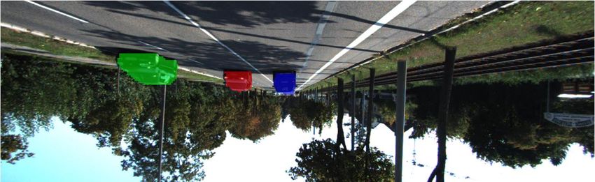
SDOD: Real-time Segmenting and Detecting 3D Object by Depth                   3

slowly. SOLO distinguish different instances by 2D location. It divided an input
image of H × W into Sx × Sy grids and do semantic segmentation in each grid;
this is similar to the main idea of YOLO. However, it only uses 2D locations to
distinguish different instances, performance not good for overlapped instances.
Therefore, we propose to solve the task by tackling three issues: 1) how to trans-
form instance segmentation tasks into semantic segmentation tasks, 2) how to
combine the 3D network with the instance network efficiently, 3) how to train
the 3D network and the instance network together.

                           Instance                                 Location
                            Depth                                  Estimation
                                                     Car   Car
                                           Car
                                                                     Corner
                           2D Bbox                                 Regression
                                       Instance-level Depth Map

                                                                                Match
                           Mask Head
                                                                                 Crop

                                           Pixel-level Depth Map

Fig. 2. SDOD Framework. SDOD consists of a backbone network and two parallel
branches: a 3D branch and a mask branch. We match and crop the instance-level
depth category map generated by the 3D branch and the pixel-level depth category
map generated by the mask branch. Finally, we will get an instance mask.

    For these problems, we use depth to connect the 3D network with the instance
network, and at the same time, use depth to transform instance segmentation
into semantic segmentation. As shown in Fig. 2, the network has been divided
into two parallel branches: the 3D branch and the mask branch. The objects’
depth discretized into depth categories, the 3D branch predicts instance-level
depth categories, and the mask branch indicates pixel-level depth categories. We
introduce the auto-annotation model trained on Cityscapes provided by Polygon-
RNN++ [1] to generate coarse masks on the KITTI dataset [8]. Then add real
depth to these coarse masks. Finally, we use these masks to train the mask
branch. Experiments on the KITTI dataset demonstrate that our network is
practical and real-time.
    In summary, in this paper we propose a framework for real-time instance
segmentation and 3D object detection. For the time to complete all tasks, it can
outperform the state-of-the-art about 1.8 times. Our contributions are three-fold:

 – Transform instance segmentation tasks into semantic segmentation tasks by
   discretion depth.
 – Propose a network that combines 3D detection and instance segmentation
   and set them as parallel branches to speed up.
 – Combine coarse masks with real depth to train the mask branch to solve
   imbalanced labels.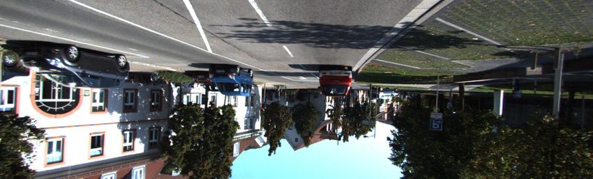
4       Li, S. et al.

2     Materials and Methods

2.1   Dataset

KITTI dataset has 7841 training images and 7581 test images with calibrated
camera parameters for 3D object detection challenges. However, due to the dif-
ficulty of instance segmentation labeling, there are only 200 labeled training
images and 200 unlabeled testing images for instance segmentation challenge.
In addition, the 3D object detection task evaluates on 3 types of targets(car,
pedestrian, cyclist), and instance segmentation task evaluates on 8 types of tar-
gets(car, pedestrian, cyclist, truck, bus, train, bicycle, motorcycle).We evaluate
cars, pedestrians, and cyclists on both 3D object detection and instance segmen-
tation tasks.
    The number of 3D objects in the KITTI dataset is slightly less than the
number of instance masks. 3D detection dataset ignores targets beyond the Lidar
detection range, and some of them are not forgotten in the instance segmentation
dataset. We take the 3D dataset as the benchmark in our work, although this
will bring some performance loss.

2.2   Instance Segmentation

It is hard to directly regress the continue center depth gd , we discretize contin-
uous depth into depth classes, and a particular class ci can be assigned to each
depth d. There are two discrete methods: linear method and non-linear method.
Linear method means that the depth d ∈ [dmin , dmax ] is linearly divided into
classes ci ∈ {c1 , c2 , ..., cK }. Note that the background is set to c0 and the value
is −1. Non-linear method chooses a more complex mapping function for dis-
cretization e.g. SDNet [22] chooses a logarithmic function and DORN chooses
an exponential function.
    Compared with the discrete linear method, the non-linear discrete method
increases the proportion of difficult examples, making the model easier to train
and converge. In this work, we spilled the depth into depth classes ci with an
exponential function 1 where K is the number of depth classes.
                                                  i−1
                                                  K−1
                                          dmax
                        ci = dmin ·                      , i ∈ {1, 2..., K}       (1)
                                          dmin

The left plot of Fig. 3 shows the linear and exponential discretization of the
depths, the right plot shows the example frequency of linear and exponential
discrete depth classes in the KITTI 3D object detection dataset. Simultaneously,
we use depth error to measure the difficulty of the depth classes, and the red
curve shows the depth class of the object is positively related to the difficulty
of the object depth estimation. The discrete exponential method increases the
proportion of hard examples, making the model easier to train and converge.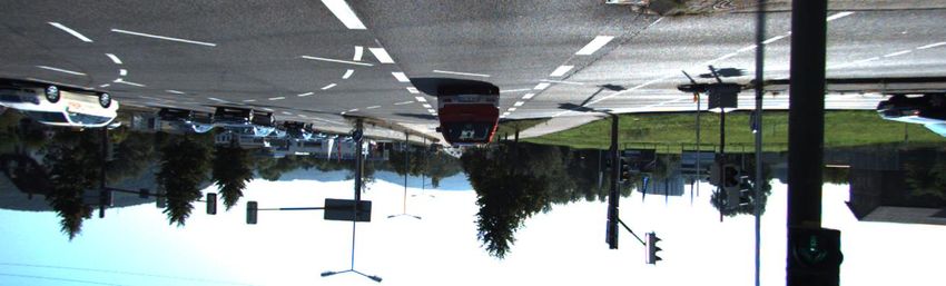
SDOD: Real-time Segmenting and Detecting 3D Object by Depth 5
Fig. 3. The left plot shows the linear and exponential discretization of the depths with
K = 80 in a depth interval [2, 80]. The right plot shows the example frequency of linear
and exponential discrete depth classes in the KITTI 3D object detection dataset. The
depth error of example in different depth classes is also shown in the right plot. The
depth error curve reflects the difficulty of the sample, and the data comes from 3DOP
[5].
2.3 3D Branch
We leverage the design of MonoGRNet, which decomposes the 3D object detec-
tion into four subnetworks: 2D detection, instance-level depth estimation, 3D
location estimation and corner regression.
We use the design of 2D detection in Multinet, which proposes a non-proposed
approach similar to YOLO and Over feat [26]. To archive the good detection per-
formance of proposal based detection systems, it uses RoiAlign in the rescaling
layer. An input image of H × W has divided into Sx × Sy grids, and each grid
is responsible for detecting objects whose center falls into the grid. Then each
grid outputs the 2D bounding box B2d and the class probabilities Pcls .
Given a grid g, this module predicts the center depth gd of the object in g
and provides it for 3D location estimation and mask branch. As shown in Fig. 2,
the module takes P5 and P3 as the input feature map. Compared with P3, P5
has a larger receptive field and lower resolution. It is less sensitive to location, so
we use P5 to generate a coarse depth estimation, and then fused with P3 to get
accurate depth estimation. We apply several parallel atrous convolutions with
different rates to get multi-scale information, then fuse it with a 2D bounding
box to generate an instance-level depth map.Compared with the mask branch’s
pixel-level depth estimation, the module output resolution is lower, which is an
instance-level. For details of implementation, please refer to section 2.4.
The 3D location module uses the 2D coordinates (u, v) and the center depth
d of the object to calculate the 3D location (x, y, z) by the following formula:
u = x · fx + cx
v = y · fy + cy (2)
d=z
fx , fy , cx, cy are camera parameters which can be obtained from the camera’s
internal parameter matrix C.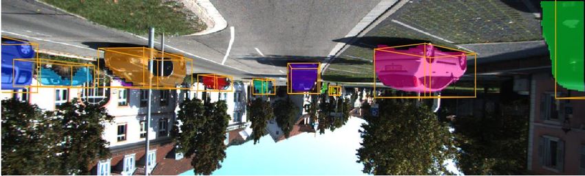
6         Li, S. et al.

    As illustrated in Fig.6, we first establish a coordinate system whose origin
is the object center, and the x ,y ,z axis is parallel to the camera coordinate
axis, and then regress the 8 corners of the object. Finally, we use the method of
Deep3DBox [21] to calculate the object’s length, width, height, and observation
angle from 8 corner points. The length, width and observation angle will be used
to calculate the depth threshold in Section 2.5.

2.4     Mask Branch

The mask branch predicts pixel-level depth categories over the entire image, and
classifies pixels based on the depth class to which they belong, which is similar to
semantic segmentation. As shown in Fig. 4, the mask branch consists of atrous
spatial pyramid pooling(ASPP) layers, fully convolutional (FCN) layers, fully
connected (FC) layers, and upsample layers. ASPP layers help to get multi-scale
information, FCN layers help to get semantic information, and FC layers help
to transform semantic information into depth information. We have tried using
convolutional layers instead of FC layers and encoding the depth category, but
the performance is not good.

ASPP The ASPP module’s input is the P5 feature map, and its resolution is
only 1/32 of the original image. To expand the receptive field of the input and
obtain more semantic information, we use the ASPP module, inspired by dilated
convolutions [?] and DeepLab v3++ [4].
   As shown in Fig. 4, The ASPP module connects 1 convolutional layer and
3 atrous convolutional layers with rates of 2,4,8. The module’s input size is
39×12×512; after upsampled and concatenated, it becomes to 156×48×256, then
we throw the feature map into FCN layers.

                                                       2D Bbox with                                Depth threshold
                      1×1
                       1×1 Conv
                           Conv                    N     category

                     3×3 Conv S = 2
          P5
                                                                                         Car
                                        1×1 Conv        FC                 H   Car
       Sx × Sy       3×3 Conv S = 4
                                                                                               N
                     3×3 Conv S = 8                                              W
                                                                                                       Match
                      Atrous Conv
                                      Upsample by 4                                                    Crop

                                                                                               H
          P3         1×1 Conv            Concat         FCN           FC
      4Sx × 4Sy                                                                      W

Fig. 4. Mask branch architecture. The mask branch consists of ASPP layers, FCN
layers, FC layers, and upsample layers. Note that the height H and width W in the
picture is 1/4 of the original input picture.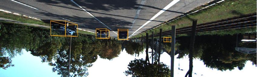
SDOD: Real-time Segmenting and Detecting 3D Object by Depth              7

FCN and FC To get a pixel-level depth category map, we use an FCN module
similar to the mask branch in Mask R-CNN, proposed by FCN [20]. As shown in
Fig 5, compared to Mask R-CNN, we have added a 1×1 convolution layer, which
is responsible for the depth classification of each pixel. K is the total number
of depth categories in equation 1; we set it to 64. The Mask branch does not
predict the pixel’s target category (car, pedestrian, cyclist); it is expected in the
3D branch. The FCN module finally outputs 1 pixel-level depth category map, as
shown in Fig. 4. The darker the pixel’s color, the greater the pixel’s depth value
and the farther the pixel is from us. The size of the output image is 312×96,
and the size of the original image is 1248×384.

Coarse Mask Generation To solve the imbalanced between mask labels
and 3D labels in the KITTI dataset, we introduce a coarse mask generated by
the auto-annotation model to increase instance segmentation samples. Polygon-
RNN++ is a state-of-the-art auto-annotation model which inputs 2D bounding
boxes and outputs instance masks. It is trained on the instance-level semantic
labeling task of the Cityscapes dataset. We use 200 labeled training images to
evaluate the accuracy of the coarse mask. Results showed in Table 1.

     Concate                                                FC     312×96
               156×48        156×48    312×96    312×96
                ×256          ×256      ×256       ×K                ×1
                        ×3        Up

Fig. 5. FCN with FC The brown feature map is obtained by 3×3 conv, and the blue
feature map is obtained by 1×1 conv. ×3 means that 3 conv layers are used. Up means
that the upsampling layer is used, and K is the total number of depth categories. We
apply fully connected layers to get the exact value of the depth category that varies
from 0 to K(background is 0). Note that the mask branch does not predict the pixel’s
target category (car, pedestrian, cyclist). It is indicated in the 3D branch.

   We did not directly train the mask branch with coarse labels , but superim-
posed the real depth value with it for training:

                        pk = ik × mk , ik ∈ [1, K] , mk ∈ {0, 1}                 (3)

ik is the real depth category of instance k, which can be calculated from equation
1. mk is the coarse mask of instance i, with a value of 0 or 1, pk is the final label
for mask branch. When training the mask branch, first, we train the mask branch
and the 3D branch together with coarse masks for 120K iterations, and then train
the mask branch only with fine masks for 40K iterations.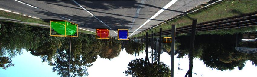
8       Li, S. et al.

Table 1. Accuracy of coarse mask generated by Polygon-RNN++. Note that Polygon-
RNN++ was trained on the Cityscapes dataset rather than the KITTI dataset.

                               car pedestrian cyclist average
                         AP 40.1      36.3      35.1     37.2
                        AP50 56.7     50.6      50.3     52.5

2.5   Match And Crop

Instance segmentation requires each pixel to be assigned to a different instance.
We need to assign each pixel in the pixel-level depth map X = {x0 , x1 , x2 ...xN −1 }
to a set of instance S = {S0 , S1 , S2 ...SM −1 } in the 3D branch,and we treat this
as a pixel matching task.
    How to match pixels with instances? There are two conditions: first, the pixel
must have the same depth category as the instance; second, the pixel must have
the same position as the instance. The following formula can describe the first
condition:

             xi ∈ Sk ⇔| xi − Sk |< δk , i ∈ [0, N − 1] , k ∈ [0, M − 1]           (4)

xi is the depth class of pixel i and xi ∈ [0, K], Sk is the depth class of the
instance k, and δk is the depth threshold of the instance k.
    As shown in Fig.6., each instance has only one depth class in the instance-level
depth map, but each instance may has multiple depth classes in the pixel-level
depth map. So we set a depth threshold δk for each instance, which is calculated
by the following formula:
                                                           ck
                        δk = (K − 1) · logdmax /dmin                              (5)
                                                       ck − 4dk

                        1                1
                4dk =     wk | cos θk | + lk | sin θk |, θk ∈ [−π, π]          (6)
                        2                2
ck is the depth class of instance k, δk is the depth margin and is shown in Fig.6.
wk , lk and θk are the width length and observation angle of the instance, which
can be obtained from the cornesr regression module. The derivation of equation
6 can be seen in the supplementary material.
    The second condition can be transformed into a crop operation. Crop op-
eration means using the 2D bounding box to crop the pixel-level depth map,
improving the mask’s accuracy. During training, we use truth bounding boxes
to crop the depth map.

2.6   Loss Function

Here we have determined independent loss functions for each module and joint
loss functions for the entire network. 2D detection includes classification loss Lcls
and box regression loss Lbox , they are defined in the same as in Multinet. Due
to the imbalance of samples between classes in the KITTI dataset, we used focal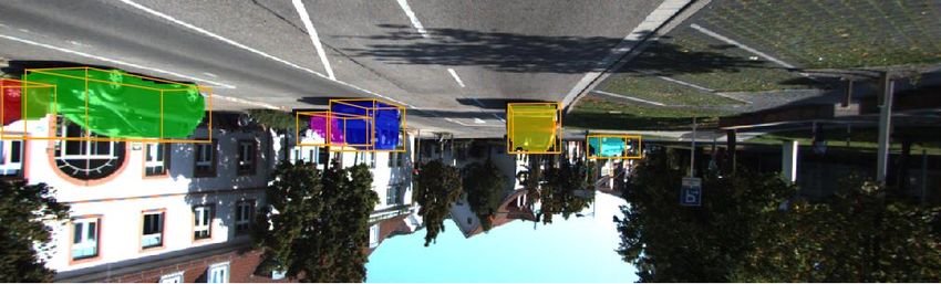
SDOD: Real-time Segmenting and Detecting 3D Object by Depth               9

                                        θ
                                                    x
                                              ∆d            h
                                    z                           l
                                                        w

                               Camera
                                              x

Fig. 6. Coordinate system and geometric constraints. The left one is a bird’s eye view
and shows the position of the target and the camera. 4d is the depth threshold and
can be calculated by equation 6 , θ is the deflection angle of the object.
loss [18] to modify the classification loss. We use L1 loss as instance-level depth
loss, corner loss and location loss, and they are the same as in MonoGRNet.
When fully connected layer is used, pixel-level depth loss is the same as the
instance-level depth loss.

                              L2d = w1 Lcls + w2 Lbox                             (7)

The total loss of 2D inspection. Where w1 and w2 are weight coefficients, when
we trained 2D detection only, we set w1 = w2 = 1.
                                        n
                                        X
                                Ld =          | di − dˆi |                        (8)
                                        i=1

Instance-level depth loss. Where n is the numbel of cell, di is the ground truth
of cell i, dˆi is the prediction of cell i.
                                         n
                                         X
                              Lmask =             | Mi − pˆi |                    (9)
                                         i=1

Pixel-level depth loss. Where n is the numbel of pixel, Mi is the ground truth of
pixel-level depth categories, which is deined by equation 3 , pi is the prediction
category of pixel i. We also tried L2 loss, CE loss and Focal loss, and finally we
found that L1 loss performed better. We think that the smaller the object is, the
farther it is, the greater its depth value is and the greater the loss is. Moreover,
this is why the long-distance object can be detected well.

2.7   Implement Details
The architecture of SDOD is shown in Figure 2. VGG-16[27] is employed as
the backbone but without the FC layers. FPN [17] is used to solve the problem
of multi-scale detection. The 2D detector should be trained first. We set w1 =
w2 = 1 in the loss functions and initialize VGG-16 with the pre-trained weights
on ImageNet. We trained a 2D detector for 150K iterations with the Adam
optimizer[13], and L2 regularization is used with a decay rate 1e-5. Then the
3D branch and the mask branch are trained for 120K iterations with the Adam
optimizer. At this stage, coarse mask generated by Polygon-RNN++ is used.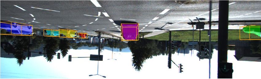
10     Li, S. et al.

Finally, we continue to train the network with fine masks for 40K iterations
with an SGD optimizer. We set the batch size to 4, learning rate to 1e-5 and
dropout rate to 0.5 throughout the training.

3    Results

The proposed network is developed using Python on a single GPU of NVidia
GTX 2080TI. For evaluating 3D detection performance, we follow the KITTI
benchmark’s official settings to evaluate the 3D Average Precision(AP3d ). For
evaluating instance segmentation performance, we follow the official settings of
the KITTI benchmark to evaluate the Average Precision on the region level
(AP ) and Average Precision with 50%(AP50 ). In this work we only evaluate
three types of objects: car, pedestrian, and cyclist. The results show that the car
has the highest accuracy and the rider has the lowest accuracy, as shown in Table
2. We compared our method with Mask R-CNN and Lklnet [9] by evaluating
the AP and AP50 of instance segmentation tasks, and the results are shown in
Table 3. Though Mask R-CNN has higher accuracy, Our approach is almost 18
times faster than that. Even if compared with the fastest two-stage instance
segmentation method, we gain about 1.8 times relative improvement on speed,
which is more suitable for autonomous driving. We also evaluated our method on
3D object detection tasks and compared with MonoFENet and MonoPSR [15].
Thanks to splitting the 3D detection into four sub-networks, we gain around 3.3
to 4.7 times relative improvement on speed, and the results are shown in Table
4.

Table 2. Specific accuracy for each category of our method. Note that our method
only evaluate AP and AP50 of car, pedestrian, and cyclist.

                             car    pedestrian cyclist average
                        AP 23.36      19.73    18.15   20.38
                       AP50 48.59     33.21    30.26   37.35

4    Discussion
In the instance-level and pixel-level depth estimation, we use equation 1 to dis-
cretize the depth into K categories. To illustrate the sensitivity to the number
of categories, we set K to different values for comparison experiments, and the
results are shown in Table5. We can see that neither too few nor too many depth
categories are rational: too few depth categories cause a large error, while too
many depth categories lose discretization.
    We apply fully connected layers to get the exact value of the depth category
that varies from 0 to K(background is 0). We try to remove the FC layer and
SDOD: Real-time Segmenting and Detecting 3D Object by Depth 11
Table 3. Instance segmentation mask AP on KITTI. Mask R-CNN is trained on the
KITTI dataset and inference with the environment of 1 core 2.5 Ghz (C/C++). All
parameters are tuned in COCO dataset in Mask R-CNN*. Ours time is the total time
of 3D detection and instance segmentation.
Method Backbone Training AP50 AP Time
Mask R-CNN ResNet101+FPN KITTI 39.14 20.26 1s
Mask R-CNN* ResNet101+FPN COCO 19.86 8.80 0.5s
Lklnet ResNet101+FPN KITTI 22.88 8.05 0.15s
Ours VGG16+FPN KITTI 37.35 20.38 0.054s
Table 4. 3D detection performance. All results is evaluated using the AP3D at 0.7 3D
IoU threshold for car class. Difficulties are define in KITTI. Ours-3D time only includes
3D inference time and does not include instance segmentation time.
Easy Moderate Hard Time
MonoFENet 8.35% 5.14% 4.10% 0.15s
MonoPSR 10.76% 7.25% 5.85% 0.20s
Ours-3D 9.63% 5.77% 4.25% 0.035s
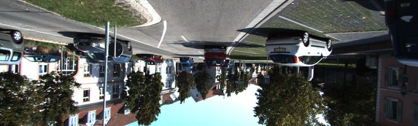
(a) Origin input image 1248*384 (b) Pixel-level depth map 312*96 (c) 3D-Mask fused output 1248*384
Fig. 7. Results Samples Results on KITTI datasets. Fig.(a) input of SDOD; Fig.(b)
pixel-level depth categories map; Fig.(c) fused instance segmentation and detection
output. We use random colors for instance segmentation. In Fig (b), the darker the
pixel’s color, the greater the pixel’s depth value, and the farther the pixel is from us.
Table 5. Ablation Study Results.
FC Depth threshold K AP AP50 Time
Y Y 32 18.90 33.23 0.049s
Y Y 64 20.38 37.35 0.054s
Y Y 96 19.84 37.34 0.058s
Y N 64 19.27 35.84 0.054s
N Y 64 18.81 32.15 0.052s12 Li, S. et al.
encode the depth category in one-hot form, e.g. if depth category is 3 just output
[1, 1, 1, 0, ..., 0]. The pixel-level feature map size is 312×96×K, and we use pixel-
wise binary cross entropy(BCE) loss to replace the L1 loss. The result is shown
in Fig.5. We can see that a fully connected layer is necessary and improves the
mask AP from 18.81 to 20.38.
To quantitatively understand SDOD for mask prediction, we perform two
error analysis. First, we replace the predicted pixel-level depth map with the
ground truth value and coarse value to evaluate the result’s mask branch’s effect.
Specifically, for each picture, we use equation 1 to convert the given masks into
a pixel-level depth map. As shown in Table 6, if we replace the predicted pixel-
level depth map with a coarse mask, the AP increase to 35.37; if we replace it
with ground truth, the AP increases to 61.18. The results show that there is still
room for improvement in the mask branch. Second, we replace the 3D predicted
results with 3D ground truth values, including 2D boxes, 3D depth values, and
depth thresholds. As reported in Table 6, the AP increase from 20.38 to 20.69;
this shows that the 3D branch has less effect on the final mask prediction.
Table 6. Error analysis.
baseline coarse mask gt mask gt 3D
AP 20.38 35.37 61.18 20.69
AP50 37.35 49.25 61.42 37.98
5 Conclusion
This paper proposes the SDOD framework to perceive complex surroundings
in real-time for autonomous vehicles. Our framework is presented to fuse 3D
detection and instance segmentation by depth, split into two parallel branches
for real-time: the 3D branch and the mask branch. We combine coarse masks with
real depth to train the mask branch to solve imbalanced labels. Our processing
speed is about 19 fps, 1.8 times faster than Lklnet and 8 times faster than Mask
R-CNN, significantly outperforms existing 3D instance segmentation methods
on tasks of segmentation and 3D detection on KITTI dataset.
6 Supplementary material: Depth Treshold Derivation
In section 3.4 match and crop, we set a depth threshold δk for each instance,
which is calculated by the following formula:
ck
δk = (K − 1) · logdmax /dmin (10)
ck − 4dk
1 1
4dk = wk | cos θk | + lk | sin θk |, θk ∈ [−π, π] (11)
2 2SDOD: Real-time Segmenting and Detecting 3D Object by Depth 13
Depth discretization In section 3.1, we spilt the depth into depth classes
ci with an exponential formula 12 where K is the number of depth classes.
Transforming formula 12 can get formula 13.
i−1
K−1
dmax
ci = dmin · , i ∈ {1, 2..., K} (12)
dmin
ci
i = 1 + (K − 1) · logdmax /dmin (13)
dmin
Depth treshold Then we prove formula 11 with formula 13. Figure 1 shows
the four possible positions of the object corresponding to the value of θ from −π
to π.
4dk = AC + AB
= OA· | cos θk | +AD· | sin θk | (14)
1 1
= wk | cos θk | + lk | sin θk |
2 2
δk = iO − iD
ciO ci
= 1 + (K − 1) · logdmax /dmin − (1 + (K − 1) · logdmax /dmin D )
dmin dmin
ciO (15)
= (K − 1) · logdmax /dmin
ciD
ck
= (K − 1) · logdmax /dmin
ck − 4dk
θ θ x
x C C C
C x O x
O O θ
O
A θ A ∆d
A
A ∆d ∆d
∆d
θ θ
B D B B D
D B D
z z z
z
Camera Camera x Camera
Camera x x x
Fig. 8. Coordinate system and geometric constraints. It shows the position of the target
and the camera. 4d is the depth threshold and can be calculated by formula 11 , θ is
the deflection angle of the object.14 Li, S. et al.
References
1. Acuna, D., Ling, H., Kar, A., Fidler, S.: Efficient interactive annotation of segmen-
tation datasets with polygon-rnn++. In: CVPR (2018)
2. Bao, W., Xu, B., Chen, Z.: Monofenet: Monocular 3d object detection with feature
enhancement networks. IEEE Transactions on Image Processing (2019)
3. Bolya, D., Zhou, C., Xiao, F., Lee, Y.J.: Yolact++: Better real-time instance seg-
mentation. arXiv preprint arXiv:1912.06218 (2019)
4. Chen, L.C., Zhu, Y., Papandreou, G., Schroff, F., Adam, H.: Encoder-decoder with
atrous separable convolution for semantic image segmentation. In: ECCV (2018)
5. Chen, X., Kundu, K., Zhu, Y., Berneshawi, A.G., Ma, H., Fidler, S., Urtasun, R.:
3d object proposals for accurate object class detection. In: NIPS (2015)
6. Chen, X., Ma, H., Wan, J., Li, B., Xia, T.: Multi-view 3d object detection network
for autonomous driving. In: CVPR (2017)
7. Fu, H., Gong, M., Wang, C., Batmanghelich, K., Tao, D.: Deep ordinal regression
network for monocular depth estimation. In: CVPR (2018)
8. Geiger, A., Lenz, P., Urtasun, R.: Are we ready for autonomous driving? the kitti
vision benchmark suite. In: ICCV (2012)
9. Girshick, R., Radosavovic, I., Gkioxari, G., Dollár, P., He, K.: Detectron. https:
//github.com/facebookresearch/detectron (2018)
10. He, K., Gkioxari, G., Dollár, P., Girshick, R.: Mask r-cnn. In: ICCV (2017)
11. Huang, Z., Huang, L., Gong, Y., Huang, C., Wang, X.: Mask scoring r-cnn. In:
CVPR (2019)
12. Kendall, A., Martirosyan, H., Dasgupta, S., Henry, P., Kennedy, R., Bachrach, A.,
Bry, A.: End-to-end learning of geometry and context for deep stereo regression.
In: ICCV (2017)
13. Kingma, D.P., Ba, J.: Adam: A method for stochastic optimization. arXiv preprint
arXiv:1412.6980 (2014)
14. Krizhevsky, A., Sutskever, I., Hinton, G.E.: Imagenet classification with deep con-
volutional neural networks. In: NIPS (2012)
15. Ku, J., Pon, A.D., Waslander, S.L.: Monocular 3d object detection leveraging ac-
curate proposals and shape reconstruction. In: CVPR (2019)
16. Li, Y., Qi, H., Dai, J., Ji, X., Wei, Y.: Fully convolutional instance-aware semantic
segmentation. In: CVPR (2017)
17. Lin, T.Y., Dollár, P., Girshick, R., He, K., Hariharan, B., Belongie, S.: Feature
pyramid networks for object detection. In: CVPR (2017)
18. Lin, T.Y., Goyal, P., Girshick, R., He, K., Dollár, P.: Focal loss for dense object
detection. In: ICCV (2017)
19. Liu, W., Anguelov, D., Erhan, D., Szegedy, C., Reed, S., Fu, C.Y., Berg, A.C.: Ssd:
Single shot multibox detector. In: ECCV (2016)
20. Long, J., Shelhamer, E., Darrell, T.: Fully convolutional networks for semantic
segmentation. In: ICCV (2015)
21. Mousavian, A., Anguelov, D., Flynn, J., Kosecka, J.: 3d bounding box estimation
using deep learning and geometry. In: CVPR (2017)
22. Ochs, M., Kretz, A., Mester, R.: Sdnet: Semantically guided depth estimation
network. In: German Conference on Pattern Recognition. pp. 288–302. Springer
(2019)
23. Qin, Z., Wang, J., Lu, Y.: Monogrnet: A geometric reasoning network for monoc-
ular 3d object localization. In: AAAI (2019)SDOD: Real-time Segmenting and Detecting 3D Object by Depth 15
24. Redmon, J., Divvala, S., Girshick, R., Farhadi, A.: You only look once: Unified,
real-time object detection. In: CVPR (2016)
25. Ren, S., He, K., Girshick, R., Sun, J.: Faster r-cnn: Towards real-time object de-
tection with region proposal networks. In: NIPS (2015)
26. Sermanet, P., Eigen, D., Zhang, X., Mathieu, M., Fergus, R., LeCun, Y.: Overfeat:
Integrated recognition, localization and detection using convolutional networks.
arXiv preprint arXiv:1312.6229 (2013)
27. Simonyan, K., Zisserman, A.: Very deep convolutional networks for large-scale
image recognition. arXiv preprint arXiv:1409.1556 (2014)
28. Teichmann, M., Weber, M., Zoellner, M., Cipolla, R., Urtasun, R.: Multinet: Real-
time joint semantic reasoning for autonomous driving. In: 2018 IEEE Intelligent
Vehicles Symposium (IV). pp. 1013–1020. IEEE (2018)
29. Tian, Z., Shen, C., Chen, H., He, T.: Fcos: Fully convolutional one-stage object
detection. In: ICCV (2019)
30. Wang, X., Kong, T., Shen, C., Jiang, Y., Li, L.: Solo: Segmenting objects by
locations. arXiv preprint arXiv:1912.04488 (2019)You can also read