ROBustness In Network (robin): an R Package for Comparison and Validation of Communities
←
→
Page content transcription
If your browser does not render page correctly, please read the page content below
C ONTRIBUTED R ESEARCH A RTICLES                                                                                        292

           ROBustness In Network (robin): an R
           Package for Comparison and Validation of
           Communities
           by Valeria Policastro, Dario Righelli, Annamaria Carissimo, Luisa Cutillo and Italia De Feis

           Abstract In network analysis, many community detection algorithms have been developed. However,
           their implementation leaves unaddressed the question of the statistical validation of the results. Here,
           we present robin (ROBustness In Network), an R package to assess the robustness of the community
           structure of a network found by one or more methods to give indications about their reliability. The
           procedure initially detects if the community structure found by a set of algorithms is statistically
           significant and then compares two selected detection algorithms on the same graph to choose the
           one that better fits the network of interest. We demonstrate the use of our package on the American
           College Football benchmark dataset.

           Introduction

           Over the last twenty years, network science has become a strategic field of research thanks to the
           strong development of high-performance computing technologies. The activity and interaction of
           thousands of elements can now be measured simultaneously, allowing us to model cellular networks,
           social networks, communication networks, power grids, and trade networks, to cite a few examples.
           Different types of data will produce different types of networks in terms of structure, connectivity,
           and complexity. In the study of complex networks, a network is said to have a community structure
           if the nodes are densely connected within groups but sparsely connected between them (Girvan
           and Newman, 2002). The inference of the community structure of a network is an important task.
           Communities allow us to create a large-scale map of a network since individual communities act
           like meta-nodes in the network, which makes its study easier. Moreover, community detection can
           predict missing links and identify false links in the network. Despite its difficulty, a huge number of
           methods for community detection have been developed to deal with different size complexity and
           made available to the scientific community by open-source software packages. In this paper, we will
           address a specific question: are the detected communities significant, or are they a result of chance
           only due to the positions of edges in the network?
               An important answer to this question is the Order Statistics Local Optimisation Method (OSLOM,
           http://www.oslom.org/) presented in Lancichinetti et al. (2011). OSLOM introduces an iterative
           technique based on the local optimization of a fitness function, the C-score (Lancichinetti et al., 2010),
           expressing the statistical significance of a cluster with respect to random fluctuations. The significance
           is evaluated by fixing a threshold parameter P a priori.
               Another interesting approach is the Extraction of Statistically Significant Communities (ESSC,
           https://github.com/jdwilson4/ESSC) technique proposed in Wilson et al. (2014). The algorithm is
           iterative and identifies statistically stable communities measuring the significance of connections
           between a single vertex and a set of vertices in undirected networks under the configuration model
           (Bender and Canfield, 1978) used as the null hypothesis. The method employs multiple testing and
           false discovery rate control to update the candidate community.
               Kojaku and Masuda (2018) introduced the QStest (https://github.com/skojaku/qstest/), a
           method to statistically test the significance of individual communities in a given network. Their
           algorithm works with different detection algorithms using a quality function that is consistent with the
           one used in community detection and takes into account the dependence of the quality function value
           on the community size. QStest assesses the statistical significance under the configuration model too.
              Very recently, He et al. (2020) suggested the Detecting statistically Significant Communities (DSC)
           method, a significance-based community detection algorithm that uses a tight upper bound on the
           p-value under the configuration model coupled with an iterative local search method.
                OSLOM, ESSC, and DSC assess the statistical significance of every single community analytically
           while QStest adopts the sampling method to calculate the p-value of a given community. Moreover,
           all of them detect statistically significant communities under the configuration model, and only QStest
           is independent of the detection algorithm.
               We present robin (ROBustness In Network), an R/CRAN package whose purpose is to give clear
           indications about the reliability of one or more community detection algorithms understudy, analyzing
           their robustness with respect to random perturbations. The idea behind robin is that if a partition

           The R Journal Vol. 13/1, June 2021                                                     ISSN 2073-4859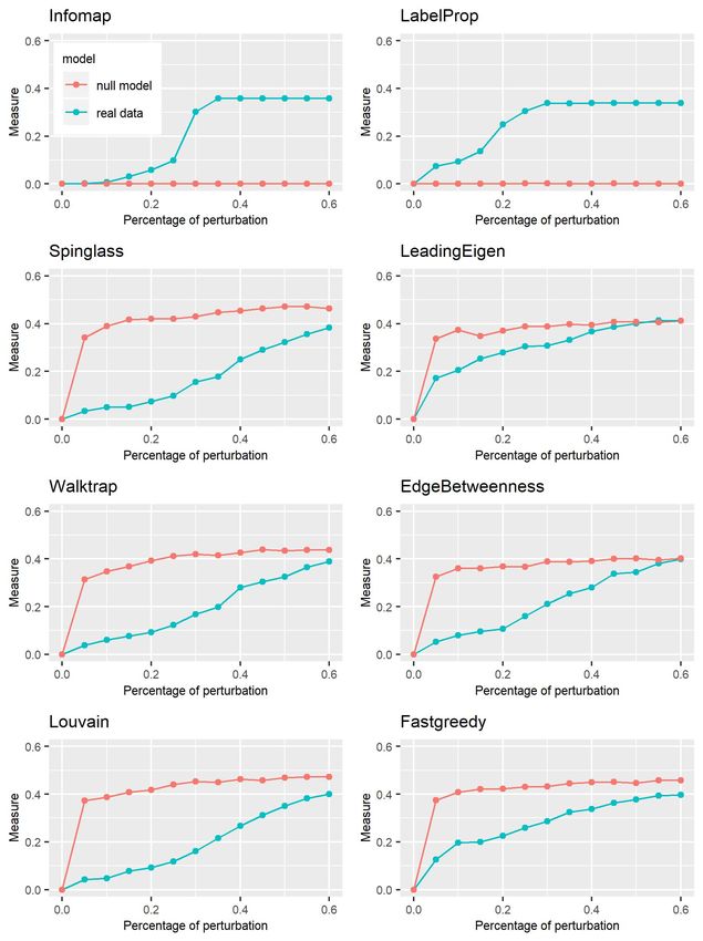
C ONTRIBUTED R ESEARCH A RTICLES                                                                                           293

           is significant, it will be recovered even if the structure of the graph is modified. Alternatively, if the
           partition is not significant, minimal modifications of the graph will be sufficient to change it. robin is
           inspired by the concept presented by Carissimo et al. (2018), who studied the stability of the recovered
           partition against random perturbations of the original graph structure using tools from Functional
           Data Analysis (FDA).
                robin provides the best choice among the variety of the existing methods for the network of interest.
           It is based on a procedure that gives the opportunity to use the community detection techniques
           implemented in the igraph package Csardi and Nepusz (2019) while providing the user with the
           possibility to include other community detection algorithms. robin initially detects if the community
           structure found by some algorithms is statistically significant, then it compares the different selected
           detection algorithms on the same network. robin assumes undirected graphs without loops and
           multiple edges.
               robin looks at the global stability of the detected partition and not of single communities but
           accepts any detection algorithm and any random model, and these aspects differentiate it from
           OSLOM, ESSC, DSC, and QStest. Unlike other studies that treat the comparison between algorithms in
           a theoretical way, such as Yang et al. (2016), robin aims to give a practical answer to such a comparison
           that can vary with the network of interest.

           The model

           robin implements a methodology that examines the stability of the recovered partition by one or more
           algorithms. The methodology is useful for two purposes: to detect if the community structure found
           is statistically significant or is a result of chance; to choose the detection algorithm that better fits the
           network under study. These are implemented following two different workflows.

               The first workflow tests the stability of the partitions found by a single community detection
           algorithm against random perturbations of the original graph structure. To address this issue, we
           specify a perturbation strategy (see subsection Perturbation strategy) and a null model to build some
           procedures based on a prefixed stability measure (see subsection Stability measure). Given:
              • a network of interest g1
              • its corresponding null random model g2
              • a Detection Algorithm (DA)
              • a stability measure (M)
           Our process builds two curves as functions of the perturbation level p, as shown in Figure 1, and tests
           their similarity by two types of functional statistical tests (see subsection Statistical tests).

                   Figure 1: Example of Mcrandom and Mc curves generated by an M stability measure

               The first curve Mc is obtained by computing M between the partition of the original network
           g1 and the partition of a different perturbed version of g1. The second curve Mcrandom is obtained
           by computing M between the partition of a null random network g2 and the partition of a different
           perturbed version of g2.
               The comparison between the two M curves enables us to reconsider the problem regarding
           the significance of the retrieved community structure in the context of stability/robustness of the

           The R Journal Vol. 13/1, June 2021                                                        ISSN 2073-4859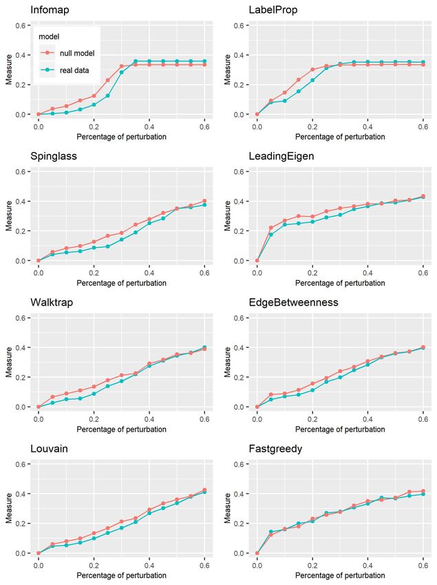
C ONTRIBUTED R ESEARCH A RTICLES                                                                                          294

           recovered partition against perturbations. The basic idea is that if small changes in the network
           cause a completely different grouping of the data, the detected communities are not reliable. For a
           better understanding of this point, we refer the reader to the paper Carissimo et al. (2018) where the
           methodology was developed.
               The choice of the null model plays a key role because we would expect it to reproduce the same
           structure of the real network but with completely random edges. For this reason, robin offers two
           possibilities: a degree preserving randomization by using the rewire function of the igraph package
           or a model chosen by the user.
               The degree preserving randomization, i.e., Configuration Model (CM), is a model able to capture
           and preserve strongly heterogeneous degree distributions often encountered in real network data
           sets and is the standard null model for empirical patterns. Nevertheless, it can happen that it is not
           sufficient to preserve only the degree of the graph understudy, so robin allows the user to include
           their own null model.
               In section Example test: the American College football network, we explore the dk null random
           model provided in Orsini et al. (2015), whose code is available at https://github.com/polcolomer/
           RandNetGen as a possible alternative to CM. The dk-series model generates a random graph preserving
           the global organization of the original network at various increasing levels of details chosen by the
           user via the setting of the parameter d. More precisely, the dk-series is a converging series of properties
           that characterize the local network structure at an increasing level of detail and define a corresponding
           series of null models or random graph ensembles. Increasing values of d capture progressively more
           properties of the network: dk 1 is equivalent to randomizing the network fixing only the degree
           sequence, dk 2 fixes additionally the degree correlations, dk 2.1 fixes also the clustering coefficient, and
           dk 2.5 the full clustering spectrum.
               The first workflow is summarised as follows (see Figure 2):

              1. find a partition C1 for the real network and a partition C2 for the null network,
              2. perturb both networks,
              3. retrieve two new partitions C1( p) and C2( p) ,
              4. calculate two clustering distances (for the real network and the null network) between the
                 original partitions and the ones obtained from the perturbed network as:

                                               M C1( p) , C1   and M C2( p) , C2                         (1)

           Steps 2) - 4) are computed at different perturbation levels p ∈ [0 : 0.05 : 0.6] to create two curves,
           one for the real network and one for the null model, then their similarity is tested by two functional
           statistical tests described in subsection Statistical tests.
             This procedure allows the filtering of the detection algorithms according to their performance.
           Moreover, the selected ones can be compared using the second workflow.

               The second workflow helps to choose among different community detection algorithms the one
           that best fits the network of interest, comparing their robustness two at a time. More precisely, the
           technique (see Figure 3):
              1. find two partitions C1 and C2 inferred by two different algorithms on the network under study,
              2. perturb the network creating a new one,
              3. retrieve two new partitions C1( p) and C2( p) ,

              4. evaluate M C1( p) , C1 and M C2( p) , C2 .

           Steps 2) - 4) are repeated at different perturbation levels p ∈ [0 : 0.05 : 0.6] to create two curves and
           then their similarity is tested.

           Perturbation strategy

           The perturbed network has been restricted to have the same number of vertices and edges as the
           original unperturbed network. Therefore, only the positions of the edges are changed. It is expected
           that if a community structure is robust, it should be stable under small perturbations of the edges.
           This is because perturbing the network edges by a small amount will imply just a small percentage of
           nodes to be moved in different communities; on the other hand, perturbing a high percentage of the
           edges in the network will produce random clusters. Note that zero perturbation p = 0 corresponds to
           the original graph while a maximal perturbation level p = 1 will correspond to the random graph.

           The R Journal Vol. 13/1, June 2021                                                       ISSN 2073-4859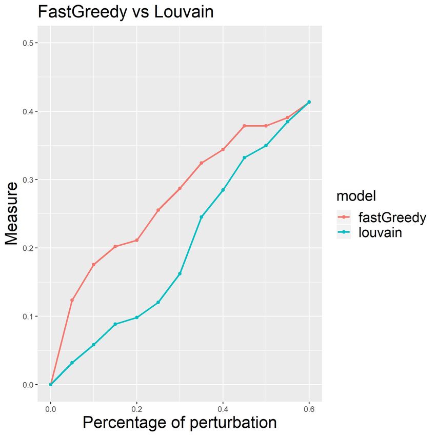
C ONTRIBUTED R ESEARCH A RTICLES                                                                                       295

                      Figure 2: Workflow to test the goodness of a community detection algorithm.

                     Figure 3: Workflow to compare two different community detection algorithms.

           Therefore, in robin, the perturbation of a network preserves the degree distribution of the original
           network.
               Two different procedures for the perturbation strategy are implemented, namely independent
           and dependent types. The independent strategy introduces a percentage p of perturbation in the
           original graph at each iteration, for p = 0, . . . , pmax . Whereas the dependent procedure introduces 5%
           of perturbation at each iteration on the previous perturbed graph, starting from the original network,
           until pmax of the graph’s edges are perturbed. In the implementation of the perturbation strategy, we
           set up pmax = 0.6, because the structure of the network becomes random if we perturb more than 50%
           of the edges.
              In particular, we noticed that the greatest modification of the network structure happens for

           The R Journal Vol. 13/1, June 2021                                                    ISSN 2073-4859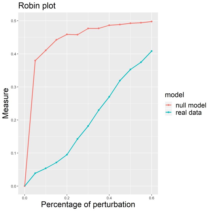
C ONTRIBUTED R ESEARCH A RTICLES                                                                                               296

           a perturbation level between 30% and 40% if a network is robust, while it happens at very low
           perturbation levels if the network is not robust.
               We stress again that the M curve for a network with a strong structure grows rapidly (perturbation
           level between 0% and 40%) then levels off when 50% < p < 100%.
              Moreover, the choice pmax = 0.6 reduces computational time and shows more clearly the differ-
           ences between the curves.
               Varying the percentage of perturbation, many graphs are generated and compared by means of
           the stability measure chosen. For each perturbation level, we generated 10 perturbed graphs and
           calculated the stability measure. From each of these graphs, we generated 9 more by rewiring an
           additional 1% of the edges. Therefore, the procedure generates 100 graphs with the respective stability
           measures for each level of p and gives as output the mean of the stability measure for every 10 graphs
           generated.

           Stability measure

           The procedure we implemented is based on four different stability measures:
               • the Variation of Information (VI) proposed by Meilǎ (2007),
               • the Normalized Mutual Information (NMI) measure proposed by Danon et al. (2005),
               • the split-join distance of van Dongen (2000),
               • the Adjusted Rand Index (ARI) by Hubert and Arabie (1985).
           VI measures the amount of information lost and gained in changing from one cluster to another, while
           split-join distance calculates the number of nodes that have to be exchanged to transform any of the
           two clusterings into the other; but for both of them, low values represent more similar clusters, and
           high values represent more different clusters. On the contrary, NMI and ARI are similarity measures,
           and therefore, lower values identify more different clusters and higher values more similar ones. To
           make all the measures comparable, we considered the 1-1 transformation for the NMI and the ARI
           since they vary between [0, 1] as:

                                                            f (X) = 1 − X                                               (2)

           Only two of the four proposed stability measures, i.e., split-join and VI, are distances. They differ in
           their dependency on the number of clusters K: while the VI distance grows logarithmically with K,
           the split-join metric grows with K toward the upper bound of 1. To make the four different stability
           measures comparable, we normalized VI and split-join between 0 and 1 (i.e., we divided the VI and
           the split-join by their maximum, respectively log (n) and 2n, where n indicates the number of vertices
           in the graph).

           Statistical tests

           robin allows different multiple statistical tests to check the differences between the real and the
           random curve or between the curves built from two different detection algorithms. The variation of p
           from 0 to 0.6 induces an intrinsic order to the data structure as in temporal data. This lets p assume,
           the same role as a time point in a temporal process, and as a consequence, we can use any suitable time
           series approach to compare our curves. In the following, we describe the use of two such approaches.
               The first is a test based on the Gaussian Process regression (GP) described in Kalaitzis and Lawrence
           (2011b). In this paper, the authors use GP to compare treatment and control profiles in biological
           time-course experiments. The main idea is to test if two time series represent the same or two different
           temporal processes. A Gaussian process is a collection of random variables, any finite number of
           which have a joint Gaussian distribution and is completely specified by its mean function and its
           covariance function, see e.g., Rasmussen and Williams (2006). Given the mean function m ( x ) and the
           covariance function k ( x, x ′ ) of a real process f ( x ), we can write the GP as:

                                                    f ( x ) ∼ GP m ( x ) , k x, x ′ .

                                                                                                                  (3)

           The random variables f = ( f ( X1 ) , . . . , f ( Xn )) T represent the value of the function f ( x ) at time
           locations ( Xi )i=1,...,n , being f ( x ) the true trajectory/profile of the gene. Assuming f ( x ) = Φ( x ) T w,
           where Φ( x ) are projection basis functions, with prior w ∼ N (0, σw       2 I ), we have

                                             m ( x ) = Φ ( x ) T E [w] = 0,    k x, x ′ = σw
                                                                                           2
                                                                                             Φ ( x)T Φ ( x)

                                                                                                                        (4)

                                                                      f ( x ) ∼ GP 0, σw 2
                                                                                           Φ ( x)T Φ ( x) .             (5)

           The R Journal Vol. 13/1, June 2021                                                           ISSN 2073-4859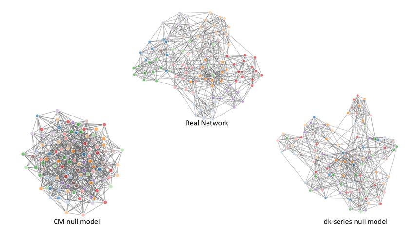
C ONTRIBUTED R ESEARCH A RTICLES                                                                                             297

           Since observations are noisy, i.e., y = Φw + ε , with Φ = (Φ( X1 ) T , . . . , Φ( Xn ) T ), assuming that the
           noise ε ∼ N (0, σn2 I) and using Eq. (4), the marginal likelihood becomes:

                                                           1                1 t −1
                                        p(y|x) =               1/2
                                                                    exp   −   y K y  y     ,                          (6)
                                                   (2π )n/2 Ky              2

                      2 ΦΦ T + σ2 I.
           with Ky = σw         n
               In this framework, the hypothesis testing problem over the perturbation interval [0, pmax ] can be
           reformulated as:
                             M1 ( x )                                             M1 ( x )
                                      ∼ GP 0, k x, x ′                                     ∼ GP m ( x ) , k x, x ′ ,

                 H0 : log2                                  against   H1 : log2                                        (7)
                             M2 ( x )                                             M2 ( x )

           where x represents the perturbation level. To compare the two curves, robin uses the Bayes Factor
           (BF), which is approximated with a log-ratio of marginal likelihoods of two GPs, each one representing
           the hypothesis of differential (the profile has a significant underlying signal) and non-differential
           expression (there is no underlying signal in the profile, just random noise).
               The second test implemented is based on the Interval Testing Procedure (ITP) described in Pini
           and Vantini (2016). The ITP provides an interval-wise nonparametric functional testing and is not only
           able to assess the equality in distribution between functions, but also to underline specific differences.
           Indeed, users can see where are localized the differences between the two curves. The Interval Testing
           Procedure is based on:
              1. Basis Expansion: functional data are projected on a functional basis (i.e. Fourier or B-splines
                 expansion);
              2. Interval-Wise Testing: statistical tests are performed on each interval of basis coefficients;
              3. Multiple Correction: for each component of the basis expansion, an adjusted p-value is computed
                 from the p-values of the tests performed in the previous step.

           In summary, GP provides a global answer on the dissimilarity of the two M curves, while ITP points
           out local changes between such curves. As a rule of thumb, we suggest initially using GP to flag
           a difference and then ITP to understand at which level of perturbation such a difference is locally
           significant.
              We also provide a global method to quantify the differences between the curves when they are
           very close. This is based on the calculation of the area under the curves with a spline approach.

           Package structure

           Installation

           Once in the R environment, it is possible to install and load the robin package with its dependencies,
           as follows:

           install.packages("robin")

               The robin package includes as dependencies igraph (Csardi and Nepusz, 2019), networkD3
           (Gandrud et al., 2017), ggplot2 (Wickham, 2019), gridExtra (Auguie, 2017), fdatest (Pini and Vantini,
           2015) , gprege (Kalaitzis and Lawrence, 2011a), and DescTools (Signorell and mult. al., 2019) packages.
           All, except gprege which is a Bioconductor package, are automatically loaded with the command:

           library(robin).

               To install the gprege package, start R and enter:

           if (!requireNamespace("BiocManager", quietly = TRUE))
                  install.packages("BiocManager")
           BiocManager::install("gprege")

           Data import and visualization

           robin is a user-friendly software providing some additional functions for data import and visualization,
           such as prepGraph, plotGraph, and plotComm. The function prepGraph, required by the procedure,
           reads, and simplifies undirected graphs removing loops and multiple edges. The available input

           The R Journal Vol. 13/1, June 2021                                                          ISSN 2073-4859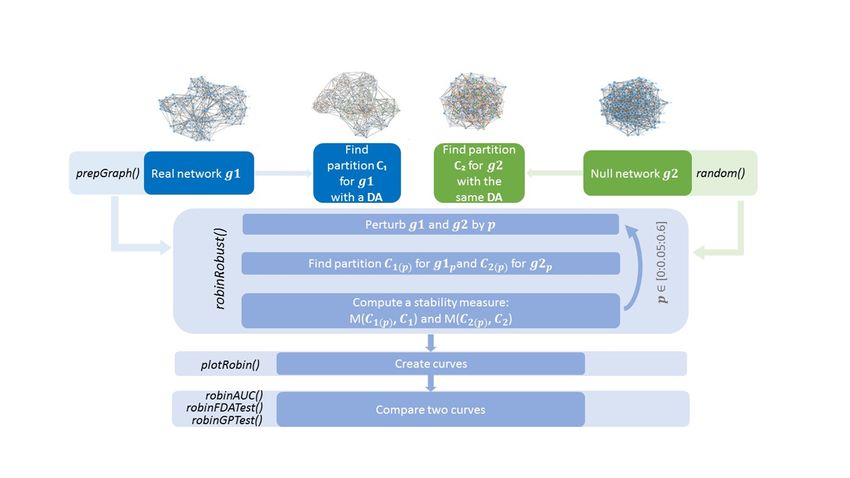
C ONTRIBUTED R ESEARCH A RTICLES                                                                                     298

           graphs formats are: “edgelist”, “pajek”, “ncol”, “lgl”, “graphml”, “dimacs”, “graphdb”, “gml”, “dl”,
           and an igraph object. The function plotGraph, with the aid of the network3D package, starting from
           an igraph object loaded with prepGraph, shows an interactive 3D graphical representation of the
           network, useful to visualize the network of interest before the analysis. Furthermore, the function
           plotComm helps to plot a graph with colorful nodes that simplifies the visualization of the detected
           communities, given the membership of the communities.

           Procedures

           robin embeds all the community detection algorithms present in igraph. They can be classified as in
           (Fortunato, 2009)
              modularity based methods:

              • cluster_fast_greedy (Clauset et al., 2005)
              • cluster_leading_eigen (Newman, 2006)
              • cluster_louvain (Blondel et al., 2008)

              divisive algorithms:

              • cluster_edge_betweenness (Newman and Girvan, 2004)

              methods based on statistical inference:

              • cluster_infomap (Rosvall and Bergstrom, 2008)

              dynamic algorithms:

              • cluster_spinglass (Reichardt and Bornholdt, 2006)
              • cluster_walktrap (Pons and Latapy, 2005)

              alternative methods:

              • cluster_label_prop (Raghavan et al., 2007).

               robin gives the possibility to input a custom external function to detect the communities. The
           user can provide his own function as a value of the parameter FUN in both analyses, implemented
           into the functions robinRobust and robinCompare. These two functions create the internal process for
           perturbation and measurement of communities stability. In particular robinRobust tests the robustness
           of a chosen detection algorithm and robinCompare compares two different detection algorithms. The
           option measure in the robinRobust and robinCompare functions provides the flexibility to choose
           between the four different measures listed in the subsection Stability measure.
              robin offers two choices for the null model to set up for robinRobust:
              • external building according to users’ preferences, then the null graph is passed as a variable,
              • generation by using the function random.
           The function random creates a random graph with the same degree distribution as the original graph,
           but with completely random edges, by using the rewire function of the igraph package with the
           keeping_degseq option that preserves the degree distribution of the original network. The function
           rewire randomly assigns a number of edges between vertices with the given degree distribution. Note
           that robin assumes undirected graphs without loops and multiple edges which are directly created,
           from any input graph, by the function prepGraph.

           Construction of curves

           The plotRobin function allows the user to generate two curves based on the computation of the chosen
           stability measures.
               When plotRobin is used on the output of robinRobust, i.e., the first step of the overall procedure,
           the first curve represents the measure between the partition of the original unperturbed graph and
           the partition of each perturbed graph (blue curve in Figure 4-Left panel), and the second curve is
           obtained in the same way but considering as the original graph the random graph (red curve in Figure
           4-Left panel). The comparison between the two curves turns the question about the significance of
           the retrieved community structure into the study of the robustness of the recovered partition against
           perturbation.

           The R Journal Vol. 13/1, June 2021                                                   ISSN 2073-4859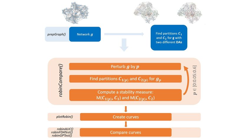
C ONTRIBUTED R ESEARCH A RTICLES                                                                                        299

               When plotRobin is used on the output of robinCompare, i.e. the second step of the overall
           procedure, it generates a plot that depicts two curves, one for each clustering algorithm. In the right
           panel of Figure 4, each curve is obtained by computing the measure between the partition of the
           original unperturbed graph with the partition of each perturbed graph, where the partition method is
           either Louvain (blue curve) or Fast Greedy (red curve).

           Figure 4: Curves of the null model and the real data generated by the VI stability measure and the
           Louvain detection algorithm on the American College Football network (Left panel). Curves of the
           Louvain and Fast greedy algorithm generated by the VI stability measure on the American College
           Football network (Right panel) (Girvan and Newman, 2002).

           Testing

           The GP test is implemented in robinGPTest and uses the R package gprege (Kalaitzis and Lawrence,
           2011a). The ITP test is implemented in robinFDATest and uses the R package fdatest (Pini and
           Vantini, 2015). The area under the curves is calculated by the function robinAUC and relies on the
           DescTools package. Figure 5 shows the curves for the comparison of Louvain and Fast greedy
           algorithms’ performance generated by the VI stability measure using the Interval Testing Procedure
           on the American College Football network (left panel) (Girvan and Newman, 2002) and corresponding
           adjusted p-values (right panel).

           Figure 5: Curves of the Louvain and Fast greedy algorithm generated by the VI stability measure using
           the Interval Testing Procedure on the American College Football network (Left panel). Corresponding
           p-values and adjusted p-values for all the intervals with the horizontal red line on to the critical value
           0.05 (Right panel).

               All the functions implemented in robin are summarized in Table 1.

           Computational time

           The time complexity of the proposed strategy, more precisely of the robinRobust function, is evaluated
           as follows. Generating a rewired network with N nodes and M edges consumes O( N + M) time, for

           The R Journal Vol. 13/1, June 2021                                                     ISSN 2073-4859
C ONTRIBUTED R ESEARCH A RTICLES 300
Table 1: Summary of the functions implemented in robin.
F UNCTION D ESCRIPTION
Import/Manipulation
prepGraph Management and preprocessing
of input graph
random Building of null model
Analysis
robinRobust Comparison of a community detection method
versus random perturbations of the original graph
robinCompare Comparison of two different
community detection methods
Visualization
methodCommunity Detection of the community structure
membershipCommunities Detection of the membership vector
of the community structure
plotGraph Graphical interactive representation
of the network
plotComm Graphical interactive representation
of the network and its communities
plotRobin Plots of the two curves
Test
robinGPTest GP test and evaluation of the Bayes factor
robinFDATest ITP test and evaluation of the adjusted p-values
robinAUC Evaluation of the area under the curve
both the real and the null model. For each network, we detect the communities, using any community
detection algorithm present in igraph or any custom external algorithm inserted by the user, and
calculate a stability measure. Let D be the time complexity associated with the community detection
algorithm chosen. The overall procedure is iterated k = 100 times for each percentage p of the
n p = 12 perturbation levels (p ∈ [0, pmax ], pmax = 0.6). In total, the proposed procedure requires
O( D + ((( N + M + D ) ∗ k) ∗ n p )) time both for the real and the null model.
In Table 2, we show the computational time evaluated on a computer with an Intel 4 GHz i7-4790K
processor and 24GB of memory. In this example, we used Louvain as a detection algorithm on the LFR
benchmark graphs (Lancichinetti et al., 2008). The time complexity could be mitigated using parallel
computing, but this is not yet implemented.
Example test: the American College football network
robin includes the American College football benchmark dataset as an analysis example that is freely
available at http://www-personal.umich.edu/~mejn/netdata/. The dataset contains the network of
United States football games between Division I colleges during the 2000 season (Girvan and Newman,
2002). It is a network of 115 vertices that represent teams (identified by their college names) and 613
The R Journal Vol. 13/1, June 2021 ISSN 2073-4859C ONTRIBUTED R ESEARCH A RTICLES 301
Table 2: Computational time
N ODES E DGES T IME ( SECS )
100 500 2.1
1000 9267 36.1
10000 100024 361.8
100000 994053 9411.6
1000000 8105913 110981.5
edges that represent regular-season games between the two teams they connect. The graph has the
ground truth, where each node has a value that indicates to which of the 12 conferences it belongs,
and this offers a good opportunity to test the ability of robin to validate the community robustness. It
is known that each conference contains around 8-12 teams. The games are more frequent between
members of the same conference than between members of different conferences. They are on average
seven between teams of the same conference and four between different ones. We applied all the
methods listed in subsection Procedures to this network, choosing as measure the VI metric.
library(robin)
my_networkC ONTRIBUTED R ESEARCH A RTICLES 302
measure="vi")
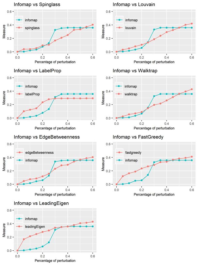
Figure 6 shows the results we obtained. If we focus on the perturbation interval [0, 0.3], it is possible
to note the similar behavior between the curves representing Infomap/Spinglass, Infomap/Louvain,
Infomap/Propagating Labels, Infomap/Walktrap, and Infomap/Edge betweenness, with a closer
distance between Infomap/Spinglass. On the contrary, the curves Infomap/Fast greedy and In-
fomap/Leading eigenvector have an opposite behavior, building almost an ellipse. This confirms
what is displayed in Table 3.
Figure 6: Plot of the VI curves of Infomap against all other methods.
In our overall procedure, we explored two different ways of generating a null model, namely the
The R Journal Vol. 13/1, June 2021 ISSN 2073-4859C ONTRIBUTED R ESEARCH A RTICLES 303
Configuration Model (CM) and the dk-series model.
graphRandomCMC ONTRIBUTED R ESEARCH A RTICLES 304
Moreover, for the dk-series model, we tested the differences between the two curves using the GP
methodology implemented in the function in robinGPTest.
BFdkC ONTRIBUTED R ESEARCH A RTICLES 305
Acknowledgements
This work was supported by the project Piattaforma Tecnologica ADVISE - Regione Campania, by the
project “TAILOR” (H2020-ICT-48 GA: 952215) and by DiSTABiF at the University of Campania Luigi
Vanvitelli that is coordinating V.P. PhD program.
Contributions
V.P. implemented the software and analyzed its properties. D.R. supported V.P. in R package imple-
mentation. A.C., L.C., and I.D.F. conceived the work, equally contributed to the development and
implementation of the concept, discussed and analyzed the results. A.C., L.C., I.D.F., and V.P. wrote
the manuscript.
Bibliography
B. Auguie. gridExtra: Miscellaneous Functions for "Grid" Graphics, 2017. URL https://CRAN.R-project.
org/package=gridExtra. R package version 2.3. [p297]
E. A. Bender and E. R. Canfield. The asymptotic number of labeled graphs with given degree sequences.
Journal of Combinatorial Theory A, 24:296–307, 1978. [p292]
V. D. Blondel, J.-L. Guillaume, R. Lambiotte, and E. Lefebvre. Fast unfolding of communities in
large networks. Journal of Statistical Mechanics: Theory and Experiment, 2008(10):P10008, 2008. doi:
10.1088/1742-5468/2008/10/p10008. [p298]
A. Carissimo, L. Cutillo, and I. De Feis. Validation of community robustness. Computational Statistics
and Data Analysis, 120:1–24, 2018. doi: 10.1016/j.csda.2017.10.006. [p293, 294]
A. Clauset, M. Newman, and C. Moore. Finding community structure in very large networks. Physical
review. E, Statistical, nonlinear, and soft matter physics, 70:066111, 2005. doi: 10.1103/PhysRevE.70.
066111. [p298]
G. Csardi and T. Nepusz. igraph: Network Analysis and Visualization, 2019. URL https://CRAN.R-
project.org/package=igraph. R package version 1.2.4.2. [p293, 297]
L. Danon, A. Díaz-Guilera, J. Duch, and A. Arenas. Comparing community structure identification.
Journal of Statistical Mechanics: Theory and Experiment, 9:219–228, 2005. doi: 10.1088/1742-5468/2005/
09/P09008. [p296]
S. Fortunato. Community detection in graphs. Physics reports, 486(3–5):75–174, 2009. [p298]
C. Gandrud, J. J. Allaire, K. Russell, and C. J. Yetman. networkD3: D3 JavaScript Network Graphs from
R, 2017. URL https://CRAN.R-project.org/package=networkD3. R package version 0.4. [p297]
M. Girvan and M. E. J. Newman. Community structure in social and biological networks. Proceedings
of the National Academy of Sciences of the United States of America, 99(12):7821–7826, 2002. doi:
10.1073/pnas.122653799. [p292, 299, 300]
Z. He, H. Liang, Z. Chen, C. Zhao, and Y. Liu. Detecting statistically significant communities. IEEE
Transactions on Knowledge and Data Engineering,, 2020. [p292]
L. Hubert and P. Arabie. Comparing partitions. Journal of Classification, 2(1):193–218, 1985. doi:
10.1007/BF01908075. [p296]
A. A. Kalaitzis and N. D. Lawrence. gprege: Gaussian Process Ranking and Estimation of Gene Ex-
pression time-series, 2011a. URL https://www.bioconductor.org/packages/release/bioc/html/
gprege.html. R package version 1.30.0; Bioconductor version 3.10. [p297, 299]
A. A. Kalaitzis and N. D. Lawrence. A simple approach to ranking differentially expressed gene
expression time courses through gaussian process regression. BMC Bioinformatics, 12(180), 2011b.
doi: 10.1186/1471-2105-12-180. [p296]
S. Kojaku and N. Masuda. A generalised significance test for individual communities in networks.
Scientific Reports, 8:7351, 2018. [p292]
The R Journal Vol. 13/1, June 2021 ISSN 2073-4859C ONTRIBUTED R ESEARCH A RTICLES 306
A. Lancichinetti, S. Fortunato, and F. Radicchi. Benchmark graphs for testing community detection
algorithms. Physical Review E, 78(4), Oct 2008. ISSN 1550-2376. doi: 10.1103/physreve.78.046110.
URL http://dx.doi.org/10.1103/PhysRevE.78.046110. [p300]
A. Lancichinetti, F. Radicchi, and J. J. Ramasco. Statistical significance of communities in networks.
Phys. Rev. E, 81:046110, 2010. [p292]
A. Lancichinetti, F. Radicchi, J. J. Ramasco, and S. F. S. Finding statistically significant communities in
networks. PloS One, 6(4):e18961, 2011. [p292]
Meilǎ. Comparing clusterings - an information based distance. Journal of Multivariate Analysis, 98(5):
873–895, 2007. doi: 10.1016/j.jmva.2006.11.013. [p296]
M. E. J. Newman. Finding community structure in networks using the eigenvectors of matrices. Phys.
Rev. E, 74(3):036104, 2006. doi: 10.1103/PhysRevE.74.036104. [p298]
M. E. J. Newman and M. Girvan. Finding and evaluating community structure in networks. Phys. Rev.
E, 69(2):026113, 2004. doi: 10.1103/PhysRevE.69.026113. [p298]
C. Orsini, M. Dankulov, P. C. de Simón, and et al. Quantifying randomness in real networks. Nature
Communications, 6(8627), 2015. doi: 10.1038/ncomms9627. [p294]
A. Pini and S. Vantini. fdatest: Interval Testing Procedure for Functional Data, 2015. URL https://CRAN.R-
project.org/package=fdatest. R package version 2.1. [p297, 299]
A. Pini and S. Vantini. The interval testing procedure: A general framework for inference in functional
data analysis. Biometrics, 72(3):835–845, 2016. doi: 10.1111/biom.12476. [p297]
P. Pons and M. Latapy. Computing communities in large networks using random walks. In Computer
and Information Sciences - ISCIS 2005, pages 284–293. Springer Berlin Heidelberg, 2005. [p298]
U. N. Raghavan, R. Albert, and S. Kumara. Near linear time algorithm to detect community structures
in large-scale networks. Phys. Rev. E, 76:036106, 2007. doi: 10.1103/PhysRevE.76.036106. [p298]
C. E. Rasmussen and C. K. I. Williams. Gaussian Process for Machine Learning. The MIT Press, 2006.
[p296]
J. Reichardt and S. Bornholdt. Statistical mechanics of community detection. Phys. Rev. E, 74:016110,
2006. doi: 10.1103/PhysRevE.74.016110. [p298]
M. Rosvall and C. T. Bergstrom. Maps of random walks on complex networks reveal community
structure. Proceedings of the National Academy of Sciences, 105(4):1118–1123, 2008. doi: 10.1073/pnas.
0706851105. [p298]
A. Signorell and mult. al. DescTools: Tools for Descriptive Statistics, 2019. URL https://CRAN.R-
project.org/package=DescTools. R package version 0.99.31. [p297]
S. van Dongen. Performance criteria for graph clustering and markov cluster experiments. Technical
report, National Research Institute for Mathematics and Computer Science in the Netherlands, P. O.
Box 94079 NL-1090 GB Amsterdam, Netherlands, 2000. [p296]
H. Wickham. ggplot2: Create Elegant Data Visualisations Using the Grammar of Graphics, 2019. URL
https://CRAN.R-project.org/package=ggplo2. R package version 3.2.1. [p297]
J. Wilson, S. Wang, P. Mucha, S. Bhamidi, and A. Nobel. A testing based extraction algorithm for
identifying significant communities in networks. The Annals of Applied Statistics, 8(3):1853–1891,
2014. [p292]
Z. Yang, R. Algesheimer, and C. J. Tessone. A comparative analysis of community detection algorithms
on artificial networks. Scientific Reports, 6(30750), 2016. doi: 10.1038/srep30750. [p293]
Valeria Policastro (package author and creator)
Dipartimento Scienze e Tecnologie Ambientali, Biologiche e Farmaceutiche
Universitá degli Studi della Campania “Luigi Vanvitelli”
Via Vivaldi, 43 81100 Caserta, Italia
and
Istituto per le Applicazioni del Calcolo “M. Picone” - sede di Napoli
Consiglio Nazionale delle Ricerche
via Pietro Castellino 111
The R Journal Vol. 13/1, June 2021 ISSN 2073-4859C ONTRIBUTED R ESEARCH A RTICLES 307
80131 Napoli, Italy
valeria.policastro@unicampania.it
Dario Righelli
Dipartimento di Statistica
Universitá di Padova
Via Cesare Battisti, 241 35121 Padova, Italia
and
Istituto per le Applicazioni del Calcolo “M. Picone” - sede di Napoli
Consiglio Nazionale delle Ricerche
via Pietro Castellino 111
80131 Napoli, Italy
d.righelli@na.iac.cnr.it
Annamaria Carissimo
Istituto per le Applicazioni del Calcolo “M. Picone” - sede di Napoli
Consiglio Nazionale delle Ricerche
via Pietro Castellino 111
80131 Napoli, Italy
Co-last and corresponding author
a.carissimo@iac.cnr.it
Luisa Cutillo
School of Mathematics
University of Leeds
Leeds
LS2 9JT, United Kingdom
and
Dipartimento di Studi Aziendali e Quantitativi
Universitá degli Studi di Napoli “Parthenope’
Via Generale Parisi, 13
80132, Napoli, Italia
Co-last and corresponding author
l.cutillo@leeds.ac.uk
Italia De Feis
Istituto per le Applicazioni del Calcolo “M. Picone” - sede di Napoli
Consiglio Nazionale delle Ricerche
via Pietro Castellino 111
80131 Napoli, Italy
Co-last and corresponding author
i.defeis@iac.cnr.it
The R Journal Vol. 13/1, June 2021 ISSN 2073-4859C ONTRIBUTED R ESEARCH A RTICLES 308
Figure 8: Plot of the VI curves of the CM null model and all the algorithms implemented.
The R Journal Vol. 13/1, June 2021 ISSN 2073-4859C ONTRIBUTED R ESEARCH A RTICLES 309
Figure 9: Plot of the VI curves of the dk-series null model with d = 2.1 and all the algorithms
implemented.
The R Journal Vol. 13/1, June 2021 ISSN 2073-4859You can also read