RIDESHARING OPTIONS FROM GEOSYNCHRONOUS TRANSFER ORBITS IN THE SUN-EARTH SYSTEM
←
→
Page content transcription
If your browser does not render page correctly, please read the page content below
AAS 21-637

             RIDESHARING OPTIONS FROM GEOSYNCHRONOUS
               TRANSFER ORBITS IN THE SUN-EARTH SYSTEM

                          Juan A. Ojeda Romero* and Kathleen C. Howell†

                Ridesharing options for secondary payloads to be delivered to regions beyond geostation-
                ary altitude are increasingly available with propulsive EELV Secondary Payload Adapter
                (ESPA) rings. However, mission design for secondary payloads faces certain challenges.
                A significant mission constraint for a secondary payload is the dropoff orbit orientation, as
                it is dependent on the primary mission. In this analysis, assume that the dropoff orbit is
                an Earth-centered Geosynchronous Transfer Orbit (GTO). Then, efficient transfers to orbits
                near the Sun-Earth L1 Lagrange point are constructed from a range of GTO orientations.
                Dynamical structures, such as stable invariant manifolds, associated with periodic and quasi-
                periodic orbits near Sun-Earth L1 are leveraged to identify and summarize types of transfer
                opportunities.

 INTRODUCTION
    Ridesharing opportunities for smallsats offer increased mission capabilities with lower launch costs. Over
 the past two decades, an increasing number of smallsats, especially cubesats, have been launched into Low
 Earth Orbit (LEO) or Geosynchronous Orbit (GEO) by exploiting ridesharing opportunities. Additionally,
 the potential to place smallsats into regions beyond GEO is facilitated by the introduction of propulsive
 Evolved Expendable Launch Vehicle (EELV) Secondary Payload Adapter (ESPA) rings. In a ridesharing
 configuration, an ESPA ring is utilized to mount a series of smallsats alongside the primary payload inside the
 launch vehicle. In this layout, the ESPA ring essentially holds and releases one or more secondary payloads,
 i.e., the smallsats, at some point along the trajectory. Propulsive ESPA rings carry an independent propulsion
 system that provides the necessary energy to place a secondary payload into regions beyond the primary
 payload orbit. The Lunar Crater and Observation and Sensing Satellite (LCROSS) spacecraft was a secondary
 payload, launched alongside the Lunar Reconnaissance Orbiter (LRO), and leveraged a propulsive ESPA
 ring to impact the Moon.1 Propulsive ESPA rings allow secondary payloads access to regions beyond GEO,
 however, variable orbit geometries and shifting launch dates present significant trajectory design challenges.
 In a ridesharing scenario, a primary payload is released from a launch vehicle into a dropoff orbit, also denoted
 as the initial secondary payload orbit, designed to meet the primary mission requirements. The geometry and
 orbital orientation of the dropoff orbit presents trajectory design challenges for secondary payloads enroute
 to other specified destinations.
    There are nearly twenty-five yearly launches to GEO that provide opportunities for ridesharing smallsats.
 Missions to GEO utilize a Geosynchronous Transfer Orbit (GTO) to reach the desired 35,786 km altitude.
 A GTO is defined as an eccentric orbit, within the context of the two-body problem, with a fixed apoapsis
 altitude at the GEO altitude. A satellite enroute to GEO is released in a GTO, the dropoff orbit in this
 investigation, from a launch vehicle and a series of maneuvers near apoapsis allows entry into a circular
 orbit at GEO. In a ridesharing scenario, a secondary payload is released along a GTO and, depending on
 the propulsive capabilitites of the payload, may access regions beyond GEO. Gershman et al. investigates
* Ph.D. Candidate, School of Aeronautics and Astronautics, Purdue University, Armstrong Hall of Engineering, 701 W. Stadium Ave.,
  West Lafayette, IN 47907-2045, jojedaro@purdue.edu
† Hsu Lo Distinguished Professor of Aeronautics and Astronautics, School of Aeronautics and Astronautics, Purdue University, Armstrong

  Hall of Engineering, 701 W. Stadium Ave., West Lafayette, IN 47907-2045, howell@purdue.edu

                                                                  1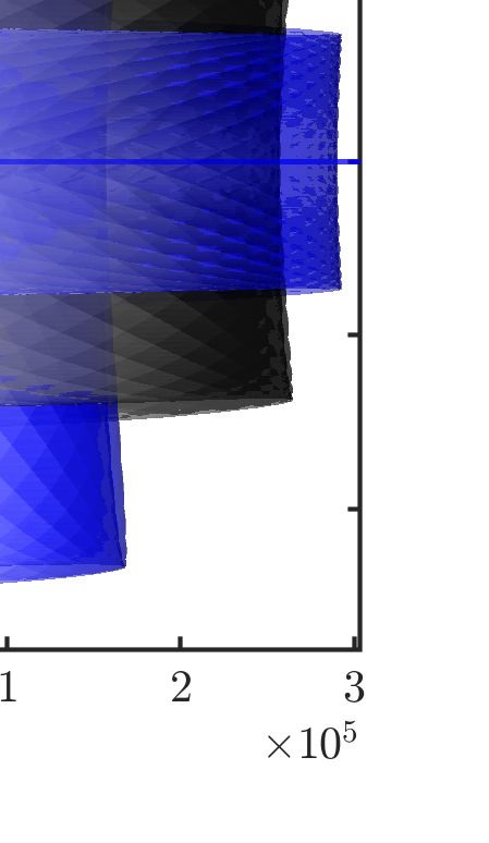
transfers from GTO to Mars and Venus with a lunar flyby.2 Fujiwara et al. examines transfers to the Moon
for a spacecraft placed in a GTO with a hybrid rocket kick motor.3 Additionally, Stender et al. presents
approximate maneuver magnitudes for mission to the Sun-Earth L1 vicinity as well as for Low Lunar Orbits
(LLO).4 In this investigation, the propulsive ESPA rings provide the necessary energy to place a secondary
payload, i.e., smallsat, beyond GEO and toward Lagrange point orbits.
   The Sun-Earth collinear Lagrange points are regions of scientific interest for secondary payloads. Sun-
Earth L1 , located between the Sun and the Earth, is an ideal region to investigate the Solar environment
while also offering favorable thermal conditions, eclipse avoidance, and continuous communications with
the Earth. However, transfers to the Sun-Earth L1 region must avoid communications interference caused by
the Sun, defined as a Solar Exclusion Zone (SEZ) region.5 The International Sun-Earth Explorer-3 (ISEE-3),
later renamed the International Cometary Explorer (ICE), was the first orbiter placed near L1 .6 The success
of the ICE mission led to the following L1 orbiters: the Advanced Composition Explorer (ACE), the Solar
Heliospheric Observatory (SOHO), and the International Physics Laboratory (WIND).5 In this investigation,
transfers from a GTO to the Sun-Earth L1 vicinity are constructed for smallsats leveraging a propulsive ESPA
ring.

BACKGROUND
   Preliminary transfer design to Sun-Earth Lagrange points is facilitated by leveraging the motion within
the Circular Restricted Three Body Model (CRTBP)7 model. The motion in the CRTBP can be generally
categorized into four types: equilibrium points, periodic solutions, quasi-periodic solutions, and chaotic.8
Periodic orbits and quasi-periodic orbits near Lagrange points, i.e., equilibrium points in the CRTBP, and
dynamical structures associated with these orbits, such as hyperbolic invariant manifolds, are leveraged to
construct efficient and flexible transfers to Sun-Earth Lagrange points.

Dynamical Model
   Insightful flow information observed in the CRTBP model is analyzed via methods from Dynamical Sys-
tems Theory (DST). The CRTBP model describes the motion of a spacecraft, P3 , with negligible mass, m3 ,
subject to the gravitational force of two larger bodies, P1 and P2 , with masses m1 and m2 , respectively.
Additionally, P1 and P2 are assumed to be in a circular orbit about their system barycenter, O. The system
is non-dimensionalized with a characteristic length, l∗ , defined as theqconstant distance between the primary
                                                                         (l )        ∗ 3
bodies, P1 and P2 , and a characteristic time, t∗ , defined as: t∗ =  G(m1 +m2 ) , where G is the universal
gravitational constant. The non-dimensional scalar equations of motion for the CRTBP are written as,

                                           ∂U ∗                    ∂U ∗              ∂U ∗
                              ẍ − 2ẏ =        ,     ÿ + 2ẋ =        ,     z̈ =        ,                          (1)
                                            ∂x                      ∂y                ∂z
                                                                                                       m2
where ∂ indicates a partial derivative, µ is the mass parameter of the system defined as µ =          m1 +m2 ,   and U ∗
is the pseudo-potential function denoted as,
                                                1−µ     µ   1
                                        U∗ =         +     + (x2 + y 2 ).                                            (2)
                                                 r13   r23  2
In Equation p(2), the distances between the spacecraft
                                                p          and P1 and P2 , i.e., r13 and r23 , respectively, are defined
as r13 = (x + µ)2 + y 2 + z 2 and r23 = (x − 1 + µ)2 + y 2 + z 2 . Note that the reference frame of the
system is a rotating frame with basis unit vectors {x̂,ŷ,ẑ} defined such that x̂ is directed from P1 towards P2 ,
ẑ is in the direction of the angular momentum vector for the P1 -P2 circular orbit, and ŷ = ẑ × x̂. The state
of the spacecraft is denoted as x̄ = [x, y, z, ẋ, ẏ, ż]T where the superscript, T , indicates a matrix transpose.
Additionally, the position and velocity vectors for P3 , in the rotating frame, are defined as r̄ = [x, y, z]T
and v̄ = [ẋ, ẏ, ż]T , respectively. The non-dimensional positions of the primary bodies P1 and P2 are fixed
at r̄1 = [−µ, 0, 0]T and r̄2 = [1 − µ, 0, 0]T , respectively. Five equilibrium solutions (Lagrange points) exist
in the x̂-ŷ plane of the rotating frame of the CRTBP model. Three collinear Lagrange points, L1−3 , lie on
the x̂ axis and two triangular Lagrange points, L4−5 , lie on vertices of an equilateral triangle created with r̄1

                                                           2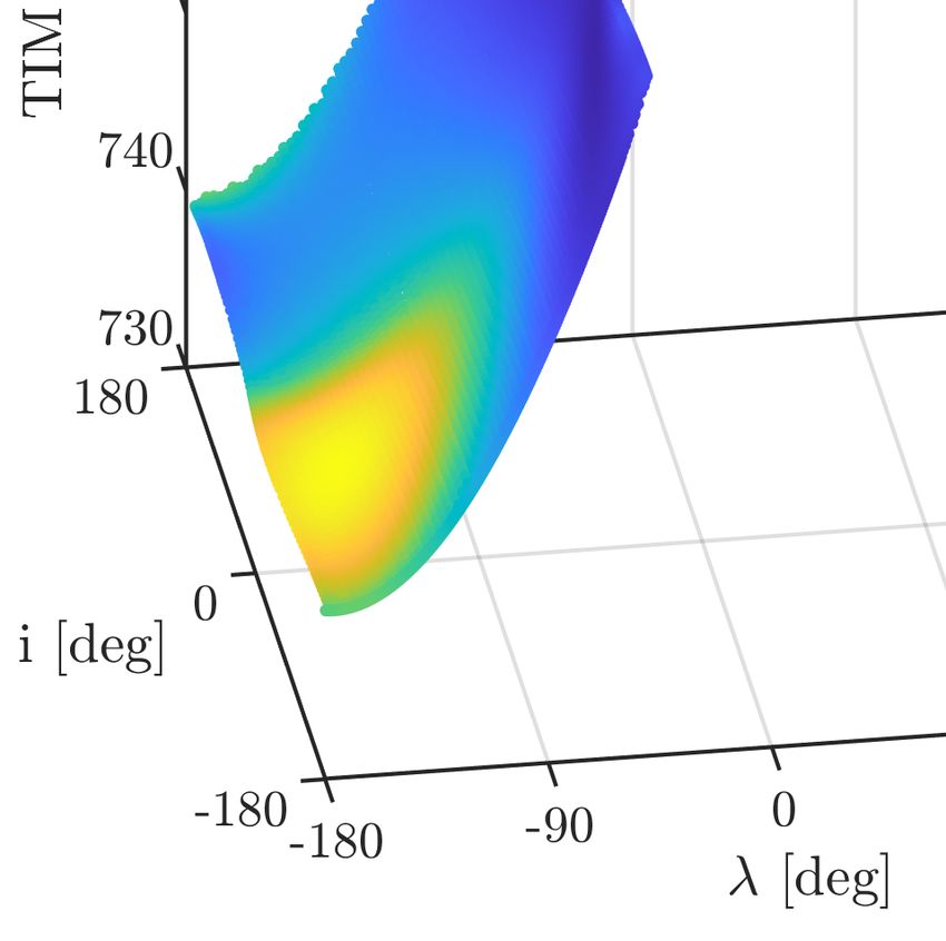
and r̄2 . An important insight from the CRTBP is the existence of an integral ofpthe motion, termed the Jacobi
Constant. The Jacobi Constant is evaluated as C = 2U ∗ − v 2 , where v = ẋ2 + ẏ 2 + ż 2 is the rotating
speed of the spacecraft. Insights from the CRTBP faciliate the search for efficient transfers in the Sun-Earth
system.

Periodic Orbits

   Periodic motion near the Lagrange points facilitates the construction of feasible transfers in the Sun-Earth
system. Periodic orbits in the CRTBP exist in one parameter families with planar Lyapunov orbits, vertical
orbits, and spatial out-of-plane halo orbits, which emanate from Lyapunov orbit families, associated with the
collinear Lagrange points, L1−3 .9 Additionally, maps, in particular stroboscopic maps, are powerful tools
for assessing the stability characteristics associated with periodic orbits. A stroboscopic map transforms a
continous time flow into a discrete time system at constant time intervals,9 or orbital periods for examination
of stability analysis of a periodic orbit. A periodic orbit on a stroboscopic map, taken at time intervals equal to
the orbit period, T , appears as a single point, x̄∗ , termed a fixed point. Linear stability analysis in the vicinity
of this fixed point reveals insightful observations concerning the flow near the periodic orbit. A monodromy
matrix, Φ(T, 0), is defined as a State Transition Matrix (STM) that relates the downstream variations in
the state to the initial state variations after one orbit period. The stability characteristics associated with
the periodic orbit are observed through the eigenvalues and eigenvectors of the monodromy matrix. The
eigenvalues, Λ,−
                 associated with periodic orbits in the CRTBP occur in reciprocal pairs,10 where the underline
refers to eigenvalues corresponding to periodic orbits. A pair of eigenvalues are equal to unity and the
remaining eigenvalues describe the local flow near the fixed point, x̄∗ , corresponding to a periodic orbit. The
existence of a center manifold associated with a periodic orbit is revealed by identifying complex eigenvalues
on the unit circle, i.e., |Λ
                           −
                             i | = 1. Complementary real eigenvalues reveal the existence of stable and unstable
manifold structures defined with |Λ    −
                                         i | < 1 and |Λ
                                                      −
                                                         i | > 1, respectively. Trajectories along the surface of the
global representations of the stable and unstable manifold structures are frequently leveraged in preliminary
mission design and serve as low-cost options that asymptotically approach, along the stable manifold, and
depart, along the unstable manifold, a periodic orbit. Additionally, the existence of quasi-periodic orbits
within the center manifold of periodic orbits offers more trajectory options to construct flexible transfers.

Quasi-Periodic Orbits

    Quasi-periodic motion observed in the vicinity of the Sun-Earth Lagrange points offer complex geometries
that facilitate the construction of efficient transfers for a range of mission design objectives. Dynamical
structures associated with periodic orbits are regularly exploited, but the behavior associated with quasi-
periodic orbits offers additional transfer opportunities and geometries. Several authors have offered strategies
to generate quasi-periodic orbits in the CRTBP.8, 11, 12 Olikara et al. categorize equilibrium points, periodic
orbits, and quasi-periodic orbits as p-dimensional invariant tori.11 The equilibrium points, i.e., Lagrange
points, are represented as 0-dimensional tori, periodic orbits as 1-dimensional tori, and quasi-periodic orbit
as q-dimensional tori with q ≥ 2. The flow for a quasi-periodic orbit densely covers the surface of the q-
dimensional torus after infinite time. In this investigation, quasi-periodic motion is represented as flow on
the surface of a q-dimensional torus, with q = 2, and a quasi-periodic orbit is constructed via a numerical
corrections scheme. The method for generating families of quasi-periodic orbits, in this analysis, originates
with Gómez and Mondelo and includes enhancements by Olikara and Scheeres.11, 13 A two-dimensional torus
is characterized by two fundamental frequencies, θ˙1 and θ˙2 , and a six-dimensional state vector on the surface
of the torus, ū, is parametrized by the angles, θ1 and θ2 , such that ū (θ1 , θ2 ). In this analysis, θ˙1 and θ˙2
are termed as the longitudinal and latitudinal frequencies, respectively. The angles, θi , are defined such that
θi (t) = θ̇i t, where t is the propagation time along the torus. From the invariant tori definition, quasi-periodic
                                                                         ˙
motion is observed for tori with irrational frequency ratios, that is θθ˙1 , and periodic motion is observed for
                                                                         2
tori when the frequency ratio is rational.
  To numerically construct a quasi-periodic orbit, the foundation is a periodic orbit in the CRTBP Sun-Earth
system represented in terms of a fixed point, x̄∗ . A stroboscopic map, generated with time T1 , is leveraged

                                                          3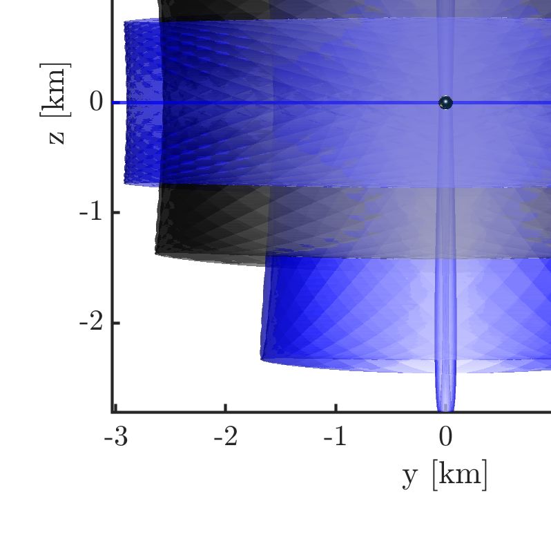
to reduce the construction of the two-dimensional torus, one that characterizes the quasi-periodic orbit, to
a search for an invariant curve. The periodic time for the stroboscopic map, i.e., T1 , is associated with the
period of the longitudinal frequency, θ˙1 , and defined as θ˙1 = 2π
                                                                 T1 . An initial state, defined as ū(θ1 (0), θ2 (0)),
is propagated along the torus and the returns to the stroboscopic map represent the invariant curve associated
with a specific quasi-periodic orbit. Additionally, a state on the surface of the two-dimensional torus, as for-
mulated in the rotating frame of the Sun-Earth CRTBP, is defined with x̄qpo = ū(θ1 , θ2 )+ x̄∗ , recalling that x̄∗
is a fixed point associated with a periodic orbit. The search for an invariant curve is mathematically described
by an invariance condition, such that a rotation matrix, R[−ρ], rotates the final state, ū(θ1 (T1 ), θ2 (T1 )), on
the torus back to its initial state, i.e.,

                             R − ρ ū θ1 (T1 ), θ2 (T1 ) − ū θ1 (0), θ2 (0) = 0̄,                                  (3)

where ū represents a row vector for the torus state. For the stroboscopic map, θ1 (0) = θ1 (T1 ), therefore,
the first return to the map occurs at θ1 (0) and the state of the first return onto the stroboscopic map, i.e.,
the final state in Equation (3), is parametrized as ū(θ1 (0), θ2 (0) + ρ), where ρ represents a rotation angle
along the invariant curve. The invariant curve, identified via implementation of the invariance condition in
Equation (3), is discretized into n torus states ūj with j = [1, ..., n] by using a truncated Fourier series. Note
that the torus states approximate the geometry of the invariant curve associated with a specific torus and the
value of n affects the accuracy of the numerical algorithm for quasi-periodic orbits. The torus states along
the invariant curve are defined as ūj (θ1 (0), θ2j (0)), where θ2j (0) ∈ [0, 2π]. Note that the torus states, ūj , are
six-dimensional vectors and the rotation matrix, R[−ρ], is a n × n real matrix evaluated with elements of the
Fourier series and the rotation angle (−ρ).11
   Quasi-periodic orbits are numerically constructed by implementing a multiple-shooting strategy along with
the invariance condition stated in Equation (3).11 In a multiple-shooting strategy, a single trajectory is divided
into a series of smaller arcs which, in a numerical corrections process, facilitate the construction of a trajec-
tory in a complex dynamical regime. Recall that the stroboscopic map that identifies the invariant curve is
constructed at sequential times such that each interval is T1 . In a multiple-shooting scheme for a torus state
propagated along the invariant curve, i.e., ūj (θ1 (0), θ2j (0)). The trajectory is subdivided into p segments,
each with an associated propagation time Tp1 . The quasi-periodic orbit, represented by a two-dimensional
torus, is now characterized by torus states, ūkj , where k = [1, ..., p]. The invariance condition, Equation
(3), is evaluated with the initial states along the invariant curve, ū1j (0, θ2j (0)) as well as the final propagated
state, i.e., the state ūpj (0, θ2j (0)) propagated by time Tp1 . Full state continuity is enforced throughout the tra-
jectory segments. Initial conditions for the corrections process are included in Olikara.11 Note that a torus
state along the invariant circle, ū1j , is expressed in terms of the phase-space, consistent with the CRTBP via
x̄Q       1      ∗                                   ∗
  j = ūj + x̄ , where, it is recalled that, x̄ is a fixed point associated with a periodic orbit. Families of
quasi-periodic orbits are constructed by enforcing constraints on the Jacobi Constant, C, the rotation angle,
ρ, or the mapping time associated with the stroboscopic map, T1 . In this investigation, quasi-periodic orbit
families at a fixed C value are constructed via pseudo-arclength continuation. The approximation of the in-
variant curve via a truncated Fourier series is not unique so additional phasing constraints are included in the
continuation process. Regions with large resonances may challenge the convergence of the multiple-shooting
algorithm, especially when generating families with a fixed C value, but anticipating these regions mitigates
the difficulties associated with this numerical algorithm.
   Stability of Quasi-Periodic Orbits Linear stability analysis offers observations concerning the local be-
havior of the flow in the vicinity of a quasi-periodic orbits. The stability properties near a fixed point asso-
ciated with a periodic orbit describe the local dynamical flow. Essentially, a stroboscopic map is constructed
with the period corresponding to the orbit. Similarly, the stability properties for quasi-periodic orbits are
observed via a linearized stroboscopic map for the invariant curve,11 i.e.,

                                             DP = R − ρ ⊗ I Φ,                                                      (4)

                                                           4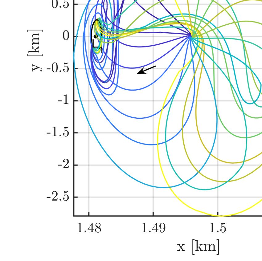
where I is a 6 × 6 identity matrix, ⊗ is the kronecker product, and Φ is a matrix, of size 6n × 6n, that includes
the STM, Φj (T1 , 0), from the torus states, ūj , along the invariant curve, such that,
Φ1 (T1 , 0) 06×6 ··· 06×6
06×6 Φ2 (T1 , 0) ··· 06×6
Φ= , (5)
.. .. ..
. . Φ (T , 0)
j 1 .
06×6 06×6 ··· Φn (T1 , 0)
where 06×6 denotes a 6 × 6 zero matrix. The eigenvalues, Λ, of the linearized map provide the stability
characteristics for the local behavior in the vicinity of a quasi-periodic orbit. The existence of a stable
manifold subspace is defined via the eigenvalues with magnitudes less than unity, i.e., kΛk < 1, and the
existence of an unstable manifold subspace is identified via kΛk > 1. The eigenvalues for each invariant
subspace, either stable or unstable, occur in concentric circles in the complex plane.14 The flow characterized
by the stable and unstable subspaces provides opportunities to construct efficient transfers into and away from
specific quasi-periodic orbits.
Invariant Manifolds for the Quasi-Periodic Orbit Trajectories that exist within the stable subspace associ-
ated with a quasi-periodic orbit offer opportunities to construct low-cost transfers to the vicinity of Sun-Earth
L1 . An infinite number of trajectories densely fill the surface of the hyperbolic stable manifold and, inherently,
these trajectories asymptotically approach the quasi-periodic orbit in reverse time. The global representation
of the stable manifold surface associated with a quasi-periodic orbit leverages an eigenvector, Ψ̄s , which
corresponds to a real eigenvalue, Λs , and the stable manifold subspace, with a zero imaginary element, such
that, Im(Λs ) = 0. Recalling that eigenvalues occur in concentric circles, an eigenvalue, Λs , with only real
parts possess a corresponding eigenvector, Ψ̄s , with real components. The eigenvector, Ψ̄s , is a vector of size
6n and is comprised of a set of sub-eigenvectors {ψ̄jS } that correspond to torus states ūj along the invariant
curve. A state on the stable manifold, x̄Sj , is approximated as,
ψ̄jS
x̄Sj = x̄Q
j ±d S k
, (6)
kψ̄rj
where ψ̄jS is the associated six-dimensional stable eigenvector for ūj also written as, ψ̄jS = [ψ̄rj
S S T
, ψ̄vj ] . The
S S S
three-dimensional vectors ψ̄rj and ψ̄vj are defined such that ψ̄rj corresponds to the elements associated with
S
position and ψ̄vj isolates the velocity elements. The eigenvectors along the full torus are evaluated from the
STM, Φ(T1 , 0).11 The global representation of the invariant stable manifold is approximated via propagation
in reverse time from the computed states in Equation (6) at a set of points around the two-dimensional torus.
DROPOFF ORBIT ORIENTATION IN THE ROTATING FRAME
The dropoff orbit orientation presents a significant design challenge for secondary payloads. A Geosyn-
chronous Transfer Orbit is an eccentric periodic orbit, within the context of the two-body problem, that
transports a primary payload to the GEO altitude. In this analysis, the GTO, i.e., the dropoff orbit, is the
departure orbit and the arrival orbit is a desired periodic or quasi-periodic orbit near the Sun-Earth L1 point.
The size of the GTO is fixed, that is, the apoapsis altitude is fixed at the GEO altitude of 35, 786 km, and
the periapsis altitude is 185 km. Note that the periapsis altitude for this analysis is a standard GTO periapsis
altitude defined by the United Launch Alliance (ULA).15 Higher altitudes can be assessed within the same
framework. The orientation of the GTO is defined via the Keplerian orbital elements: Ω, ω, and i, defined in
McClain16 and the departure location is the GTO periapsis. In a ridesharing scenario, the dropoff orbit orien-
tation is dictated by the primary mission constraints, therefore, in this analysis, it is assumed that there is no
a priori information about the GTO, i.e., the dropoff orbit, orientation. In this investigation, a change in GTO
orientation is described as a change in the position of the GTO periapsis, i.e., the departure location. The
position of the GTO periapsis, r̄dep , is described with Keplerian orbital elements associated with the J2000
Earth Mean Equatorial (EME) inertial reference frame, but the target periodic and quasi-periodic orbits exist
in the rotating frame of the Sun-Earth CRTBP model. The GTO departure position in the EME frame, i r̄dep ,
5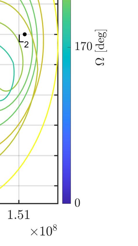
is parameterized via the traditional Keplerian orbital elements, Ω, ω, and i i, see McClain;16 note that i i is the
inclination of the orbit in the EME frame. In the Sun-Earth rotating frame, the GTO departure position, r r̄dep ,
is parameterized via the angles, λ and δ, as illustrated in Figure 1(b), such that the departure position, at a
fixed altitude, is represented as r r̄dep (λ, δ). In this analysis, the parameters that describe the GTO departure
position in the inertial frame are defined in Table 1 and a comparison of the Keplerian orbital elements in the
inertial frame and the rotating frames angles, λ and δ, is plotted in Figure 2. For a range of departure epochs,

                             (a)                                                  (b)

     Figure 1: (a) J2000 Earth Mean Equatorial inertial reference frame, denoted with {X̂,Ŷ ,Ẑ},
      and the Sun-Earth rotating frame, with basis vectors {x̂,ŷ,ẑ} (b) GTO periapsis departure
        position, expressed in the Sun-Earth rotating frame, parameterized by angles: λ and δ

                             (a)                                                  (b)

       Figure 2: (a) Rotating frame inclination, r i, and (b) δ angles at varying epoch dates and Ω
            angles. The values of r i and δ are formulated in the Sun-Earth rotating frame

                                                        6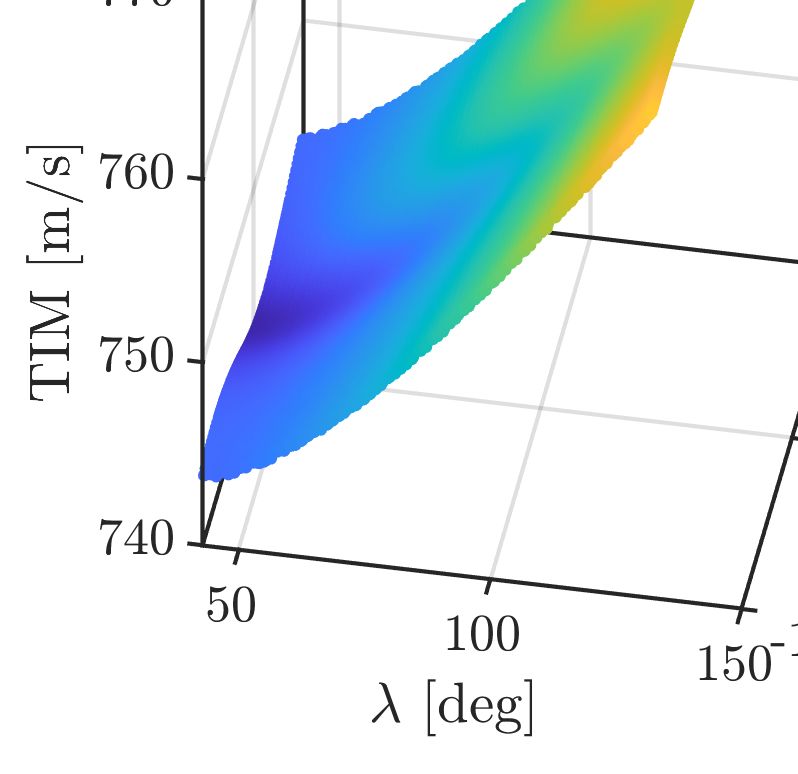
the GTO departure position, r r̄dep , varies in the Sun-Earth rotating frame as i r̄dep remains constant in the
EME frame. In this investigation, the objective is the construction of transfers at a fixed departure epoch from
a range of orientations. The range of orientations is described via a changing Ω angle in the EME frame with
a fixed inclination, i i, and ω (refer to Table 1). The plots in Figure 2 present the varying inclination in the
rotating frame, r i, and the angle δ, defined in Figure 1(b), for a range of epochs and Ω values. The rotating
inclination, r i, values plotted in Figure 2(a) possess a range: |i i − isun | < r i < |i i + isun |, where isun is
the inclination of the ecliptic in the EME frame, as illustrated in Figure 1(a). Note that the inclination of the
ecliptic, isun , varies with epoch, however, the variation is small such that, in this investigation, the inclination
is defined as: isun = 23.43◦ . Additionally, the range of the δ values, illustrated in Figure 1(b) and plotted
in Figure 2(b), is denoted: −isun < δ < isun . The range of δ plotted in Figure 2(b) and presented in Table
1 is only applicable for a fixed ω value. In this investigation, optimal ∆V transfers are constructed over a
range of orientations from a departure epoch of: June 2, 2022 12:00:00.000, with the variation of the rotating
frame inclination, r i, and the δ angles plotted as a red line in Figure 2. An understanding of the variable GTO
departure positions, i.e., the varying orientations, facilitates the search and construction of efficient transfers
to the vicinity of the Sun-Earth L1 Lagrange point.

     Table 1: Comparison of variables that parameterize the GTO periapsis position in the J2000
                            EME inertial and Sun-Earth rotating frame

                                Inertial Frame                Rotating Frame
                               ra = 35, 786 km               ra = 35, 786 km
                                 rp = 185 km                   rp = 185 km
                                   i
                                     i = 27◦         |i i − isun | < r i < |i i + isun |
                               0◦ < Ω < 360◦                −isun < δ < isun
                                    ω = 0◦                    0◦ < λ < 360◦

TRANSFERS WITH A DEEP SPACE MANEUVER
   Transfers leveraging the trajectories along the surface of the stable manifold corresponding to periodic and
quasi-periodic orbits and incorporating a single deep space maneuver (DSM) offer advantageous options over
a range of departure positions near the Earth. Transfers with a single DSM are constructed by connecting a
trajectory along the surface of the stable manifold associated with a periodic, or quasi-periodic, orbit and a
bridging arc from a departure position near the Earth. Figure 3 illustrates a transfer into a periodic orbit near
the Sun-Earth L1 point with a stable manifold trajectory arc, plotted in cyan, and a bridging arc, plotted in
black. The transfer arcs in Figure 3 are propagated in reverse time, that is, the motion of the spacecraft is

   Figure 3: Transfer with single Deep Space Maneuver into a general periodic orbit. Transfer arcs
                                   are propagated in reverse time

from an arrival location on the periodic orbit, i.e., an injection point, to the departure position at the GTO
periapsis near Earth. Note that the injection point, x̄inj , into a periodic orbit can be parameterized by the

                                                         7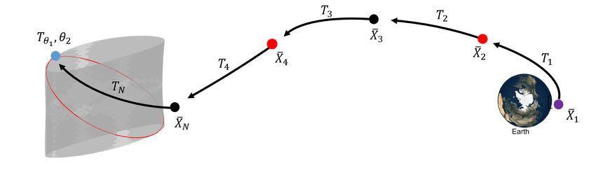
time variable: τ . For transfers into quasi-periodic orbits, that is, orbits constructed from a two-dimensional
torus, the injection point, x̄inj , is parameterized by two components: Tθ1 and θ2 , where Tθ1 is a time along
the orbit, analogous to the longitudinal time along the torus, and θ2 is a location along the invariant curve.
Two options for the DSM, the vector ∆V̄ in Figure 3, are explored in this analysis: a tangent maneuver and
a general maneuver, both impulsive. Recalling that in Figure 3, the spacecraft is propagated in reverse time,
the DSM is an impulsive maneuver implemented at the end of the bridging arc and the initiation of the stable
manifold arc. For a tangent burn DSM, the maneuver is assumed to be directed along the velocity vector at the
final state along the bridging arc and can, therefore, be defined via the scalar magnitude, ∆Vtan . A transfer
with a general impulsive DSM possesses maneuver components defined as: ∆V̄gen = [∆Vx , ∆Vy , ∆Vz ]T ,
and are also introduced at the end of the bridging arc. Observe that a state along a manifold structure, either
stable or unstable, associated with a periodic and quasi-periodic orbit can be parameterized by two and three
variables, respectively. Recall that a state in the CRTBP model is defined as a six-dimensional vector. For
periodic orbits, the injection point, x̄inj , is evaluated by propagating from an initial state, x̄0 , on the orbit
by time τ . From the periodic orbit injection point, a state on the stable manifold is constructed, as detailed
by Bosanac,8 and the state is propagated in reverse time, TM . In this process, the initial state on the orbit,
x̄0 , is fixed and it is assumed that a state along the global representation of the stable manifold surface
can be approximated. Only two variables, τ and TM , are required to locate a state on the stable manifold
structure associated with a periodic orbit and, additionally, two variables are also necessary to parameterize
states along the unstable manifold structure. For quasi-periodic orbits, the injection point, x̄inj , is computed
by propagating a state along the invariance curve, x̄inv (θ2 ), through time Tθ1 . The invariant curve state,
x̄inv (θ2 ), is parameterized by the angle θ2 and is evaluated with the truncated Fourier series utilized in the
invariance condition corrections process. For states along the stable manifold structures associated with
quasi-periodic orbits, the variables θ2 , Tθ1 , and TM , describe the state along the global representation of the
manifold. In describing an end state for a transfer, i.e., x̄f , with a tangent burn into a periodic orbit, also
plotted in Figure 3, only four variables are required: τ , TM , ∆Vtan , Tarc . These variables are termed the
fundamental variables for the transfer. To address convergence issues near dynamically complex regions, the
transfer arcs, i.e., the stable manifold arc and the bridging arc, are subdivided into a series of segments, that
is, reformulated into a multiple-shooting problem. However, the number of fundamental variables does not
change, that is, the end state along the transfer is always described with the same number of fundamental
variables. The fundamental variables for single DSM transfers into periodic and quasi-periodic orbits are
summarized in Table 2. In this investigation, two constraints are enforced at the end state, i.e., x̄f , of the
transfer: an altitude and an apsis constraint. Note that the end state along the transfer is essentially the
departure state at periapsis for a GTO with a fixed size, i.e., fixed periapsis and apoapsis altitude. Therefore,
the GTO departure position is parameterized by two angles: λ and δ, as illustrated in Figure 1(b). In this
investigation, the constraints for the DSM transfers are written as:
Altitude Constraint : r̄f − r̄dep (λ, δ) = 0,
(7)
Apsis Constraint : (r̄f − r̄e ) · v̄f = 0,
where r̄f and v̄f are the final end state position and velocity along the transfer, r̄e is the position of the
Earth with respect to the Sun-Earth barycenter in the CRTBP rotating frame, and the desired GTO departure
position, r̄dep is defined as:
cos(λ) cos(δ)
r̄dep (λ, δ) = r̄e + halt sin(λ) cos(δ) , (8)
sin(δ)
with halt as the fixed GTO periapsis altitude such that: halt = 185 km. Two additional free variables are
introduced to the transfer problem: λ and δ with the formulation of the constraint conditions in Equation (7)
as a four-dimensional column vector. For example, transfers into a periodic orbit with a general maneuver,
i.e., scenario B from Table 2, requires six fundamental variables: τ , TM , ∆Vx , ∆Vy , ∆Vz , Tarc . In all
transfer scenarios, only the end state apsis and altitude constraints are enforced, that is, the constraint vector
for the transfer problem is two-dimensional. However, with the constraint conditions from Equation (7), the
constraint is written as a four-dimensional vector with two additional free variables, λ and δ, included in
the transfer problem. The reformulation of the constraint vector and introduction of the free variables, λ
8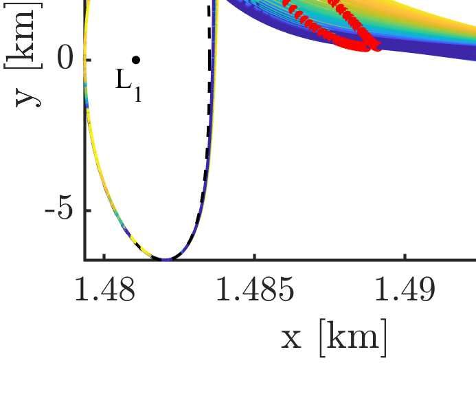
and δ, permits more control over the departure position. Additionally, the reformulation of the constraint
condition does not affect the solution space for the DSM transfer problem, summarized in Table 2. The
dimension of the solution space applicable to the DSM transfer is evaluated as the difference between the
number of fundamental variables and the number of constraints. For example, transfers with a tangential
DSM to a periodic orbit appear on a two-dimensional surface of solutions. Information regarding surface
shape and terminal conditions, e.g., if the surface is closed, is not known a priori or not known as a closed
form function. The scenarios in Table 2 are applicable for transfers leveraging either stable and unstable
manifold structures and a bridging arc. Transfers in the solution space for the scenarios in Table 2 offer
advantageous options for mission design in the Sun-Earth system.

    Table 2: Fundamental variables and constraints for different DSM type transfers into periodic
                                     and quasi-periodic orbits

                                                     Fundamental           DSM          Departure         Dimension of
     Scenario              Target
                                                      Variables            Type         Constraints      Solution Space
                                                                          Tangent        Altitude
         A            Periodic Orbit                  τ, TM , TArc                                             2
                                                                          (∆Vtan )        Apsis
                                                                          General        Altitude
         B            Periodic Orbit                  τ, TM , TArc                                             4
                                                                          (∆V̄gen )       Apsis
                                                                          Tangent        Altitude
         C         Quasi-Periodic Orbit            Tθ1 , θ2 , TM , TArc                                        3
                                                                          (∆Vtan )        Apsis
                                                                          General        Altitude
         D         Quasi-Periodic Orbit            Tθ1 , θ2 , TM , TArc                                        5
                                                                          (∆V̄gen )       Apsis

SOLAR EXCLUSION ZONE PATH CONSTRAINT
   Communications constraints, in the form of a path constraint, for transfers to the Sun-Earth L1 vicinity
must be included in the preliminary design process. Communications constraints during the Earth-to-L1
transfer and along the L1 Lagrange point orbit require that the spacecraft avoid crossing in front of the solar
disk when viewed from the Earth.5 In the rotating frame of the Sun-Earth system, a Sun-Earth-Vehicle (SEV)
angle, α, is defined as the angle between the position of the spacecraft with respect to the Earth, r̄23 , and the
negative x̂-axis direction, as illustrated in Figure 4. The vector r̄23 is defined as: r̄23 = r̄ − r̄e , where r̄ and r̄e
are the position vectors of the spacecraft and the Earth measured from the Sun-Earth barycenter, respectively,
-x̂ = [−1, 0, 0]T , and r̄e = [1 − µ, 0, 0]T . The SEV angle is defined:

                                                           r̄23 · −x̂
                                              α = cos−1                 ,                                            (9)
                                                             kr̄23 k

where Ā · B̄ is the vector dot product in this formulation. The Solar Exclusion Zone (SEZ), plotted in Figure
4, is a region defined by a right circular cone with the vertex at the Earth and a constant SEV angle, αSEZ .
The communications constraint must be enforced along the transfer path and a mathematical definition for a
general path constraint is formulated as,
                                    N Z
                                    X         Ti
                         Fpath =                   Fp2 (x̄i (t)) − |Fp (x̄i (t)) |Fp (x̄i (t)) dt = 0,                    (10)
                                     i    0

where | · | implies an absolute value. The path constraint condition in Equation (10) is similar to the formu-
lation from Ojeda Romero et al.,17 but the form in Equation (10) has smooth first order partial derivative,
i.e., the partial derivative is defined everywhere along the trajectory arcs. In Equation (10), the transfer is
formulated as a multiple-shooting problem and applicable over N nodes along the trajectory where Ti is
the propagation time for the ith arc. The path constraint formulation is versatile and may be applied at arc
segments near the constraint region, i.e., the SEZ cone. The general path constraint formulation in Equation

                                                                 9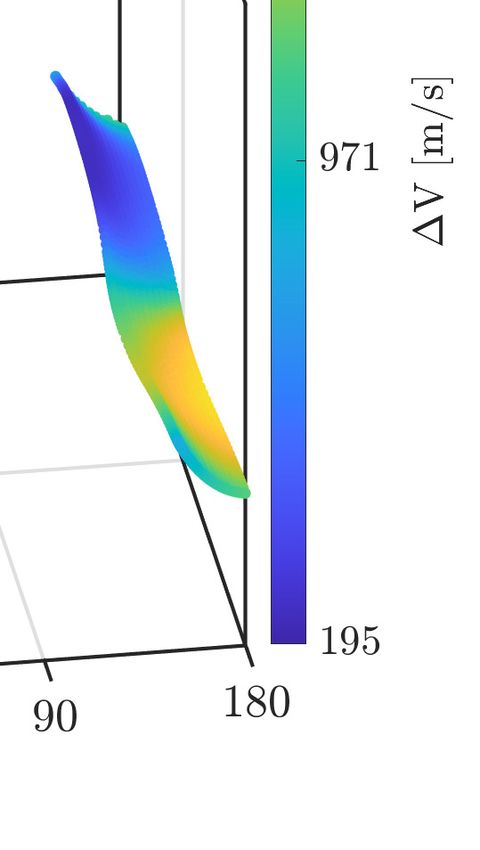
Figure 4: Solar Exclusion Zone defined in the Sun-Earth rotating frame (red). The fixed angle
                                αSEZ defines the size of this region

(10) is implemented in this investigation to prevent crossing into the SEZ for L1 transfers. The function that
expresses the SEZ crossing condition is defined as,

                                         Fp = sin (α (x̄i (t)) − αSEZ ) ,                                      (11)

such that, the SEV angle, α, and the position with respect to the Earth, r̄23 , are functions of the state, x̄i (t),
that corresponds to the state node, x̄i , propagated by time t. A trapezoidal numerical integration scheme,
consistent with the Trapz function in MATLAB, is implemented for the general path constraint in Equation
(10). An important observation is that the general path constraint function in Equation (10) is compatible
with any path constraint condition that can be formulated as an inequality Fp ≥ 0.

TRANSFERS INTO PERIODIC ORBITS FROM GTO
   Transfers into a halo orbit near the Sun-Earth L1 Lagrange point are constructed with stable manifold tra-
jectories and a DSM that is tangent to the path. The SOHO mission5 leveraged a periodic halo orbit near
the Sun-Earth L1 point to avoid crossing into the SEZ. The halo orbit selected for the SOHO mission em-
ployed the following amplitudes: x-amplitude of 206, 448 km, y-amplitude of 66, 672 km, and z-amplitude
of 120, 000 km.5 The halo orbit is a southern halo orbit, i.e., the motion of the spacecraft as viewed by an
observer at the Earth is counterclockwise, with a period of 180 days. Recall that the objective is the construc-
tion of efficient transfers from a GTO with a fixed periapsis altitude at 185 km with no a priori information
about the GTO orientation. The secondary spacecraft departure state, x̄dep , is at the GTO periapsis and, from
Figure 1(b), is parameterized by angles λ and δ. Transfers with a tangential DSM, i.e., scenario A in Table 2,
are identified as potential transfer options into the southern halo orbit from different departure positions near
the Earth. Although transfers described by both scenarios A and B are applicable for the periodic halo orbit,
transfer scenario A is selected for the two-dimensional solution space. Recall that in scenario A from Table
2, the end point location is also the departure position of the GTO, r̄dep in Figure 3, at different near-Earth
positions. Additionally, the departure position is constrained to be on the x̂-ŷ plane of the Sun-Earth rotating
frame, i.e., δ = 0◦ . The additional constraint decreases the solution space for the transfers with tangent
DSMs by one, therefore, all transfer solutions into the periodic halo orbit with a departure state along the x̂-ŷ
plane near Earth appear on a one-dimensional curve of solutions.
   A curve of solutions that represents transfers into a southern L1 halo orbit with a tangential DSM is con-
structed via a multiple-shooting corrections algorithm. The transfer scenario illustrated in Figure 3 is formu-
lated as a multiple-shooting problem by further subdividing the stable manifold arcs and the bridging arcs.
Full state continuity is enforced along the subarcs that belong to the stable manifold arc segment as well as
the bridging arc segment. Recall that, in reformulating the transfer problem into a multiple-shooting problem,
the dimension of the solution space does not change and the multiple-shooting formulation only aids in the
corrections process. An initial guess is generated by utilizing a Poincaré map, as plotted in Figure 5. The
trajectories along the surface of the stable manifold that emanates from the southern L1 halo orbit are prop-

                                                        10
agated in reverse time to a surface of section defined as a plane, i.e., x = 1.48x10⁸ km, and their crossings
onto the map are plotted in blue in Figure 5. The bridging arc trajectories, i.e., the red points in Figure 5, are
Stable Manifold Crossings
Bridging Arc Crossings
Figure 5: Poincaré map of stable manifold crossings from southern halo orbit (blue) and
bridging arc crossing (red) onto the cross-section. Two star points indicate the chosen stable
manifold arc and bridging arc to construct an initial guess
propagated forward in time from a location near the Earth, i.e., the departure position corresponding to the
GTO periapsis, towards the surface of section. The bridging arc trajectories are propagated from a location
near Earth that corresponds to λ = 0◦ and δ = 0◦ . In the map in Figure 5, only two dimensions are displayed,
y and z, and there is no information about the velocity along the trajectories. For this scenario, an initial guess
is selected by identifying intersections between the stable manifold crossings and the bridging arc crossings,
i.e., the black stars in Figure 5. Recall that the solutions space for this scenario is two-dimensional and,
therefore, the transfers with a tangent maneuver are contained on a two-dimensional surface. However, for
simplicity the focus of the analysis is constructing transfers originating from different locations along the
GTO near the Earth and initiated in the Ecliptic plane, i.e., the x̂-ŷ plane of the Sun-Earth rotating frame. An
additional departure constraint is added to scenario A in Table 2, δ = 0◦ . The tangent maneuver transfers are
now all captured along a one-dimensional curve of solutions. Figures 6(a) and 7(a) display curves of transfer
solutions for a range of λ values.
(a) (b)
Figure 6: (a) Curve of transfer solutions into a southern halo orbit with a tangent DSM. (b)
Selected transfers with the location of the DSM in red and the location of the injection points into
halo orbit in magenta
A selected range of transfers, i.e., corresponding to the box in red in Figure 6(a), is plotted in Figure 6(b).
The transfers presented in Figure 7(b) correspond to the transfers in Figure 7(a). Positive ∆V magnitudes
for the DSM, presented in Figures 6-7, correspond to prograde burns and negative ∆V values are retrograde
11(a) (b)
Figure 7: (a) Curve of transfer solutions into southern halo orbit with a tangent DSM. (b)
Transfers into a southern halo orbit with the location of DSM in red and the location of injection
points into halo orbit in magenta
burns. Note the different locations of the injection points, in magenta, into the southern halo orbit and the
maneuver locations along the transfers, in red, in Figures 6(b) and 7(b). The curves in Figures 6-7 indicate
that the departure position from the GTO towards the specific southern L1 halo orbit can be placed along any
point around the Earth.
TRANSFERS INTO QUASI-PERIODIC ORBITS FROM GTO
Trajectories into quasi-periodic orbits in the vicinity of the Sun-Earth L1 Lagrange point are constructed
by including a DSM along the transfer. In this example, transfers to quasi-periodic Lissajous orbits near L1
are constructed with trajectories along the stable manifold structure associated with a Lissajous orbit and a
bridging arc segment. This example is identified as either scenario C, a tangent maneuver transfer, or scenario
D, a general maneuver transfer, from Table 2. Mission requirements, such as maximum/minimum SEV, α,
constraints, may restrict a set of applicable quasi-periodic orbits for a secondary spacecraft.
A ’tighter’ Lissajous orbit, similar to the op-
ertational orbits of the ACE5 or the Deep Space
Climate Observatory (DSCVR)18 missions, is of-
ten selected to maintain specific science or com-
munications requirements. In this application, a
quasi-periodic orbit with characteristics similar to
that designed for the ACE spacecraft is selected
as the target destination. The ACE spacecraft is
in an L1 Lissajous orbit with approximate x-, y-,
and z-amplitudes of 81, 755 km, 264, 071 km, and
154, 406 km, respectively.5 An orbit with similar
amplitudes is selected from a family of Lissajous or-
bits constructed employing a fixed Jacobi Constant
value, C = 3.000876398, in the Sun-Earth system.
In Figure 8, specific members of the fixed Jacobi
Constant family, plotted in blue, are projected onto
the ŷ-ẑ plane, while the selected Lissajous orbit is
depicted in black. A communications constraint im- Figure 8: Family of Lissajous orbits constructed
posed on the ACE spacecraft requires the trajectory at a fixed Jacobi Constant
to remain outside the Solar Exclusion Zone, defined
12as αSEZ = 5◦ and illustrated in Figure 4, for this investigation. Stationkeeping (STK) strategies have been
developed and implemented to maintain the Lissajous trajectory beyond the SEZ; however, the focus of this
application is the transfer into a Lissajous orbit at an ideal location, i.e., an injection point, that will maxi-
mize the time outside the SEZ before an STK maneuver is necessary. The search for an injection point that
maximizes time outside the SEZ is formulated as the search for an angle, θ2 , along the invariant curve. An
injection point along a quasi-periodic orbit is parameterized by Tθ1 and θ2 , where Tθ1 is the propagation time
from a point along the invariant curve and θ2 is an angle along the invariant curve, such that: x̄inj (Tθ1 , θ2 ).
Recall that an injection point is computed by propagating a state along the invariant curve, i.e., x̄inv (θ2 ), over
time, Tθ1 . The state along the invariant curve is defined as: x̄inv (θ2 ) = x̄∗ + ū(0, θ2 ), where x̄∗ is the fixed
point of a periodic orbit associated with the quasi-periodic family and ū is a six-dimensional torus state. In
the search for an ideal injection point, the propagation time is assumed to be zero, Tθ1 = 0, that is, the ideal
injection point is dependent on the angle θ2 . The state along the invariant curve, x̄inv (θ2 ), is propagated
along the Lissajous orbit and the SEV angle, α, is illustrated in Figure 4. The computation of a trajectory arc
along a quasi-periodic orbit is consistent with the following steps:
1. Identify an initial angle, θ20 , along the invariant curve. Create the state along the invariant curve:
x̄0inv = x̄∗ + ū(0, θ20 ). Recall that x̄∗ is a fixed point associated with a periodic orbit used in the
quasi-periodic orbit corrections process.
2. Propagate the current state, x̄0inv , with the mapping time, T1 , associated with the quasi-periodic orbit.
3. Identify the next state along the invariant curve. The next angle along the invariant curve is: θ21 =
θ20 + ρ, where ρ is the rotation angle corresponding to the quasi-periodic orbit. Calculate the new state,
x̄1inv = x̄∗ + ū(0, θ21 ).
4. Propagate the new state, x̄1inv , with the mapping time T1 .
5. Connect the beginning of the trajectory from x̄1inv to the end of the trajectory from x̄0inv .
6. Repeat steps 3-5 for any number of revolutions around the quasi-periodic orbit.
Note that this representation of the quasi-periodic trajectory utilizes the approximation of the invariant curve
from a truncated Fourier series. The time beyond the SEZ threshold for a set of revolutions on the Lissajous
trajectory corresponding to a range of θ2 values with 13 revolutions is plotted in Figure 9(a). Points A and B
identified in Figure 9(a) correspond to the θ2 angles: 152.85◦ and 335.35◦ , respectively. The trajectories that
emerge from the identified injection points with the maximum time above the SEZ threshold, αSEZ = 5◦ ,
before crossing into the SEZ cone. In Figure 9(a), several points in red, i.e., trajectories along the Lissajous
orbit, are defined by even longer intervals outside the SEZ than trajectories indicated by points A and B.
However, trajectories corresponding to the red points initially violate the SEZ cone, therefore, these injections
points are not viable for consideration. The characterization of the invariant curve is not unique, therefore the
θ2 values in Figure 9(a) are dependent on the characterization of the invariant curve via the truncated Fourier
series. The trajectory for point B appears in a polar plot in Figure 9(b) with the SEZ illustrated by a dashed
red line. The angular dimension for the polar plot corresponds to an angle ζ defined as ζ = tan−1 yz ,
computed with the y- and z-components of a state along a Lissajous trajectory, and the radial direction is the
SEV angle α, defined in Equation (9).
Poincaré maps are leveraged to determine an initial guess, i.e., a single DSM transfer, constructed lever-
aging the stable manifold structures associated with a Lissajous orbit and a bridging arc segment. The con-
struction of a transfer into a quasi-periodic orbit, i.e., a Lissajous orbit, is essentially scenarios C and D from
Table 2. In this analysis, a transfer with a single general DSM originating from a GTO periapsis position near
Earth is consistent with scenario D which, from Table 2, has a five-dimensional solution space. Recall that the
objective of this example is to enter into an ideal injection point along a Lissajous orbit, that is, a fixed value
of Tθ1 and θ2 . Therefore, the solution space consistent with this scenario is reduced to a three-dimensional
surface. Additionally, for simplicity, the focus is the identification of transfers originating from different
13A B =120° =60°
Injection Point
=180° =0°
L1
10°
Violation Point
=240° =300°
(a) (b)
Figure 9: (a) Time above 5◦ threshold. Points in red are trajectories that initially violate the
threshold. (b) Trajectory for injection point corresponding to θ2 = 335.35◦ . The red dashed line
corresponds to αSEZ = 5◦ cone.
near-Earth positions along the ecliptic, i.e., the x̂-ŷ plane of the Sun-Earth rotating frame. This condition is
satisfied via the introduction of the constraint δ = 0◦ . Recall that the constraint conditions in Equation (7)
are reformulated for scenarios A-D in Table 2 and two additional variables, λ and δ, corresponding to the
departure position, are included in the transfer problem. The fundamental variables for transfer scenario D
are: Tθ1 , θ2 , TM , TA , ∆Vx , ∆Vy , ∆Vz , λ, and δ. Note that the added variables do not change the solution
space. Finally, the solution space for transfers with a general DSM that insert into an ideal injection point
along a Lissajous orbit from a GTO periapsis position along the Sun-Earth ecliptic is two-dimensional. To
generate an initial guess for the single general DSM transfers, the trajectories on the surface of the stable
manifold corresponding to the Lissajous orbit are propagated in reverse time towards a surface of section.
The position vector of the GTO departure position is a function of δ and λ as illustrated in Figure 1(b), with a
fixed altitude, 185 km, with respect to the Earth. The GTO periapsis is situated along the Sun-Earth x̂ line on
the opposite side of the Sun and Earth; such a location corresponds to δ = 0◦ and λ = 0◦ . The initial guess
for the velocity vector associated with the departure positions, i.e., the bridging arc segment, is constructed
by applying a maneuver ∆V in a direction perpendicular to the radial direction of the GTO periapsis; note
that the radial direction is with respect to the Earth. The direction of the departure velocity vector varies such
that a set of bridging arc transfers is generated when the states are forward propagated towards a surface of
section. A surface of section, defined as y = 2.69x10⁵ km in the rotating frame, is selected to produce the
initial conditions and generate a single DSM transfer. The points in red in Figure 10(a) are the second returns
to the surface of section from a set of bridging arcs, propagated in forward time from the GTO departure
position, and the blue points correspond to the stable manifold trajectories, propagated in reverse time from
the Lissajous injection points. An initial guess is produced with a pair of blue and red points that are close in
position in the x̂-ẑ projection and is plotted in Figure 10(b). The initial guess is reformulated into a multiple
shooting problem and corrected via a Newton predictor-corrector algorithm.
The solution space for a transfer into a Lissajous orbit with a single maneuver is constructed via a numerical
continuation scheme. In Figure 9(a), the values of θ2 = 335.35◦ , 152.85◦ are identified as desired injection
points with Tθ1 = 0 into the selected Lissajous orbit. The initial guess in Figure 10(b), from a fixed λ and
δ, is divided into a series of discontinuous arcs, consistent with a multiple shooting scheme, and a feasible
solution is constructed via a Newton predictor-corrector algorithm. Recall that the trajectories, consistent with
scenarios in Table 2, are propagated in reverse time and a single general DSM is performed, as illustrated
in Figure 3. The objective is the construction of the two-dimensional solution surface of transfers from the
14(a) (b)
Figure 10: (a) Poincaré map for trajectories along the stable manifold (blue) and connecting arcs
(red). The selected initial guess is depicted by the black circle (b) Selected initial guess
GTO departure positions along the Sun-Earth ecliptic. The selected initial guesses in Figure 10(b) do not
correspond to the ideal injection locations, i.e., θ2 = 335.35◦ , 152.85◦ . The first step is a transfer into
one of the two possible ideal injection locations. By reformulating the constraint conditions in scenario D
in Table 2 with Equation (7), the fundamental variables for the transfer are: Tθ1 , θ2 , TM , TArc , λ, δ, and
∆V̄gen , where ∆V̄gen = [∆Vx , ∆Vy , ∆Vz ]T . There are nine free variables and two departure constraints
corresponding to: apsis and altitude. Note that the departure conditions, via Equation (7), are defined as
a four-dimensional vector. The goal is a search for a transfer into a desired injection point, defined by θ2 ,
therefore, four fundamental variables, Tθ1 , TM , λ, and δ, remain constant so the solution space representing
the transfers is a one-dimensional curve. A pseudo-arclength continuation strategy is leveraged to create a
curve of transfers with varying θ2 and TArc values. A curve can also be generated by fixing any combination
of two free variables from Tθ1 , TM , and Tarc with the fixed λ and δ angles. A curve of transfers is displayed
in Figure 11(a). This curve is not a complete representation of the solution space and the only point of interest
152.85° 335.35°
(a) (b)
Figure 11: (a) Initial guess curve - search for θ2 (b) Solution curve for fixed θ2 = 335.35◦ and
Tarc
is a transfer with corresponding θ2 = 335.35◦ or 152.85◦ ; one such instance is identified in Figure 11(a). The
time outside the SEZ reported in Figure 9(a) corresponds to a trajectory with Tθ1 = 0, therefore the transfer
15from 11(a) is utilized as an initial point to generate a separate curve with varying Tθ1 and TM . To construct
the curve in Figure 11(b), λ, δ, and θ2 are fixed along with one of the following variables: TM or TArc .
Two points on the solution curve in Figure 11(b) possess the desired Tθ1 = 0. Finally, a surface of transfers
is generated from the sample transfer with the desired θ2 and Tθ1 values, i.e., the values that correspond
to the desired injection point on the Lissajous orbit. The surface, or family of transfers, is created through
pseudo-arclength continuation process by fixing θ2 and Tθ1 , and one of the following variables: TM , TArc ,
and λ. Recall that the objective is an exploration of the solution space for all possible GTO orientations and,
in this application, only transfers such that the departure is from a GTO periapsis located along the Sun-Earth
ecliptic are considered, i.e. δ = 0◦ . The enclosed transfer solution surface for a region around the Earth, such
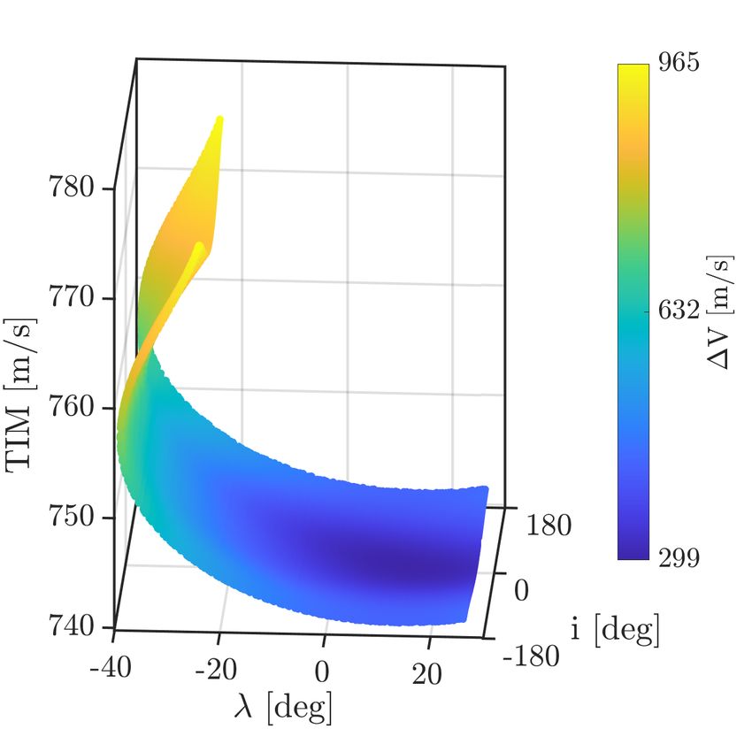
that −40◦ ≤ λ ≤ 20◦ is depicted in Figure 12(a). Note that, in Figure 12, Tmani tot tot
and Tarc are the total time
along the stable manifold and bridging arc transfer segments, respectively. In the transfer scenarios presented
in Table 2, there is no information about the maneuver implemented at the GTO periapsis; a Transfer Injection
Maneuver (TIM) is necessary to shift from the GTO departure position to the transfers on the solution curve,
e.g., Figure 12(b).
(a) (b)
Figure 12: (a) Solution Surface from a region corresponding to −40◦ ≤ λ ≤ 20◦ near the Earth.
(b) Solution Surface with GTO inclination and Transfer Injection Maneuvers (TIMs).
A summary of the steps to generate the solution surface for this example follows:
1. Identify injection location, θ2 , along the invariant curve of a quasi-periodic orbit.
2. Fix the departure location from Earth, i.e., fix λ and δ. Note that the departure location is an apsis with
respect to the Earth with a fixed altitude.
3. Generate transfer arcs from the fixed departure location towards a surface of section.
4. Generate stable manifold trajectories from the desired quasi-periodic orbit. These are propagated in
reverse time toward a surface of section.
5. Identify an initial guess from a Poincaré map constructed via the crossings onto the surface of section.
6. Search for a solution with the desired θ2 . A continuation strategy is implemented by fixing any combi-
nation of two from the variables: Tθ1 , TM , TArc along with λ and δ.
167. Search for the solution with desired Tθ1 = 0, by fixing θ2 , λ, δ and either TM or TArc .
8. Explore the solution space for a fixed Tθ1 , θ2 , δ. The surface is created from a series of curves created
from a continuation strategy. The curve is created by fixing one of the variables: TM , TArc , or λ.
These steps can be generalized to search the solution space for any single DSM transfer to a specific quasi-
periodic orbit. A separate solution surface is constructed from the previous steps for a different initial depar-
ture position near the Earth, for example, given λ = 90◦ and for δ = 0◦ , see Figure 13(a), and λ = 180◦ and
δ = 0◦ in Figure 14(a). Recall that every point on this surface corresponds to a single maneuver transfer.
(a) (b)
Figure 13: (a) Solution Surface from a region corresponding to 40◦ ≤ λ ≤ 130◦ near the Earth.
(b) GTO inclination and Transfer Injection Maneuvers (TIMs) information.
(a) (b)
Figure 14: (a) Solution Surface for direct transfers. (b) Solution Surface with GTO inclination
and Transfer Injection Maneuvers (TIMs).
17You can also read