Raising context awareness in motion forecasting
←
→
Page content transcription
If your browser does not render page correctly, please read the page content below
Raising context awareness in motion forecasting

                                                      Hédi Ben-Younes*,1 , Éloi Zablocki*,1 , Mickaël Chen1 , Patrick Pérez1 , Matthieu Cord1,2
                                                                                      1
                                                                                          Valeo.ai, 2 Sorbonne Université
                                                {hedi.ben-younes,eloi.zablocki,mickael.chen,patrick.perez,matthieu.cord}@valeo.com
arXiv:2109.08048v2 [cs.CV] 21 Apr 2022

                                                                    Abstract                               formances when the scene information about the agent’s
                                                                                                           surroundings is removed from the input (see section 4). This
                                            Learning-based trajectory prediction models have en-           phenomenon stems from the very strong auto-correlations
                                         countered great success, with the promise of leveraging           often exhibited in trajectories [6, 10]. For instance, when
                                         contextual information in addition to motion history. Yet, we     a vehicle is driving straight with a constant speed over the
                                         find that state-of-the-art forecasting methods tend to overly     last seconds, situations in which the vehicle keeps driving
                                         rely on the agent’s current dynamics, failing to exploit the      straight with a constant speed are overwhelmingly repre-
                                         semantic contextual cues provided at its input. To alleviate      sented; similarly, if a vehicle starts braking, its future path is
                                         this issue, we introduce CAB, a motion forecasting model          very likely a stopping trajectory. As a consequence, models
                                         equipped with a training procedure designed to promote the        tend to converge to a local minimum consisting in forecast-
                                         use of semantic contextual information. We also introduce         ing motion based on correlations with the past motion cues
                                         two novel metrics — dispersion and convergence-to-range           only, failing to take advantage of the available contextual
                                         — to measure the temporal consistency of successive fore-         information [3,11,15,25]. For example, in Figure 1, we ob-
                                         casts, which we found missing in standard metrics. Our            serve that several predictions made by the Trajectron++ [42]
                                         method is evaluated on the widely adopted nuScenes Pre-           model leave the driveable area which hints that the scene in-
                                         diction benchmark as well as on a subset of the most diffi-       formation was not correctly used by the model.
                                         cult examples from this benchmark. The code is available
                                                                                                               Such biased models relying too much on motion corre-
                                         at github.com/valeoai/CAB.
                                                                                                           lation and ignoring the scene information are unsatisfactory
                                                                                                           for several reasons. First, context holds crucial elements to
                                                                                                           perform good predictions when the target trajectory is not
                                         1. Introduction                                                   an extrapolation of the past motion. Indeed, a biased model
                                             Autonomous systems require an acute understanding of          will likely fail to forecast high-level behavior changes (e.g.
                                         other agents’ intention to plan and act safely, and the ca-       start braking), when scene information is especially needed
                                         pacity to accurately forecast the motion of surrounding           because of some event occurring in the surroundings (e.g.
                                         agents is paramount to achieving this [3,4,49]. Historically,     front vehicle starts braking). Leveraging context is thus
                                         physics-based approaches have been developed to achieve           paramount for motion anticipation, i.e. converging quickly
                                         these forecasts [27]. Over the last years, the paradigm has       and smoothly towards the ground truth ahead in time. Fur-
                                         shifted towards learning-based models [37,42]. These mod-         thermore, a biased model has a flawed reasoning because
                                         els generally operate over two sources of information: (1)        it bases its predictions on motion signals rather than the
                                         scene information about the agent’s surroundings, e.g. Li-        underlying causes contained within the scene environment.
                                         DAR point clouds [7, 8, 29, 36] or bird-eye-view rasters          For example, when applied on a vehicle that has started to
                                         [8, 21, 29, 37, 42], and (2) motion cues of the agent, e.g. its   decelerate, it will attribute its forecast on the past trajec-
                                         instantaneous velocity, acceleration, and yaw rate [12, 37]       tory (e.g. ‘The car will stop because it has started brak-
                                         or its previous trajectory [9, 22, 35, 42]. But despite being     ing.’) instead of the underlying reason (e.g. ‘The car will
                                         trained with diverse modalities as input, we remark that,         stop because it is approaching an intersection with heavy
                                         in practice, these models tend to base their predictions on       traffic.’) [33, 47]. As a direct consequence, explainability
                                         only one modality: the previous dynamics of the agent. In-        methods analyzing a biased model can lead to less satisfac-
                                         deed, trajectory forecasting models obtain very similar per-      tory justifications. Overall, it is thus paramount for motion
                                                                                                           forecasting algorithms to efficiently leverage the contextual
                                           * equal   contribution                                          information and to ground motion forecasts on it.
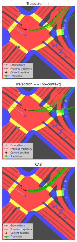
Figure 1. Predictions from a) CAB
                                                                                                  (ours), b) Trajectron++, and c) Tra-
                                                                                                  jectron++ without the context input.
                                                                                                  The thickness of trajectories represent
                                                                                                  their likelihood. Trajectron++ and its
                                                                                                  blind variant have very similar pre-
                                                                                                  dictions and they both forecast tra-
                                                                                                  jectories that leave the driveable area.
                                                                                                  CAB is more consistent with the map.
         (a) CAB (ours)                (b) Trajectron++           (c) Trajectron++ (no-context)   Sidewalks are in blue, crosswalks in
                                                                                                  yellow and driveable areas in red.

    In this paper, we propose to equip a motion forecast-             ral stability of successive predictions and their spatial con-
ing model with a novel learning mechanism that encour-                vergence speed.
ages predictions to rely more on the scene information, i.e.              To validate the design of our approach, we conduct ex-
a bird-eye-view map of the surroundings and the relation-             periments on nuScenes [6], a public self-driving car dataset
ships with neighboring agents. Specifically, we introduce             focused on urban driving. We show that we outperform
blind predictions, i.e. predictions obtained with past mo-            previous works [42, 52], as well as the alternative debias-
tions of the agent only, without any contextual informa-              ing strategies that we propose, inspired by the recent lit-
tion. In contrast, the main model has access to both these            erature in Visual Question Answering (VQA) and Natural
inputs but is encouraged to produce motion forecasts that             Language Inference (NLI) [5, 31]. Besides, we use Shap-
are different from the blind predictions, thus promoting the          ley values to measure the contribution of each modality on
use of contextual information. Our model is called ‘CAB’              the predictions: this allows us to measure how well a model
as it raises Context Awareness by leveraging Blind predic-            can leverage the context input. Lastly, we conduct evalua-
tions. It is built on the Conditional Variational AutoEncoder         tions on a subset of the most difficult examples of nuScenes
(CVAE) framework, widely used in motion forecasting; in               where we find that our approach is better suited to anticipate
practice, it is instantiated with the Trajectron++ [42] trajec-       high-level behavior changes.
tory forecasting backbone. Specifically, CAB acts on the
probabilistic latent representation of the CVAE and encour-           2. Related Work
ages the latent distribution for the motion forecasts to be
different to the latent distribution for the blind predictions.           Motion forecasting models aim to predict the future tra-
Additionally, we introduce Reweight, and RUBiZ, two al-               jectories of road agents. This prediction is achieved us-
ternative de-biasing strategies that are not specific to proba-       ing information from their current motion such as veloc-
bilistic forecasting models as they rely on loss and gradients        ity, acceleration or previous trajectory, and some contex-
reweighting respectively.                                             tual elements about the scene. This context can take var-
    In motion forecast algorithms deployed in real robotic            ious forms, ranging from raw LiDAR point clouds [7, 8,
systems, when successive forecasts are done, it is desirable          26, 29, 36, 39, 40] and RGB camera stream [26, 30, 41, 45]
to have both a fast convergence towards the ground-truth, as          to more semantic representations including High-Definition
well as a high consistency of consecutive predictions. Ac-            maps [3,8,16,17,21,29,37,42,43,51], or detections of other
cordingly, we introduce two novel metrics: convergence-to-            agents and their motion information [12, 35, 37, 42]. Re-
range and dispersion. These metrics aim at providing more             cent trajectory prediction models are designed to produce
refined measurements of how early models are able to an-              multiple forecasts, attempting to capture the multiplicity of
ticipate their trajectory and how stable through time their           possible futures [12, 24, 46]. Various learning setups are
successive predictions are.                                           explored to train these models: regression in the trajectory
                                                                      space [9,12,14,20], spatio-temporal occupancy map predic-
    Overall, our main contributions are as follows.
                                                                      tion [3, 16, 17, 43, 49], or probabilistic methods with either
    1. We target the problem of incorporating contextual in-          implicit modelling using Generative Adversarial Networks
formation into motion forecasting architectures, as we find           (GANs) [18, 19, 41, 51], or explicit modelling with Condi-
that state-of-the-art models overly rely on motion.                   tional Variational Auto-Encoder (CVAE) [21,26,40,42,44].
    2. We present CAB, an end-to-end learning scheme that             Our work is based on this CVAE family of methods, which
leverages blind predictions to promote the use of context.            not only has provided strong results in motion forecasting
    3. In addition to standard evaluation practices, we               but also structurally defines a separation between high-level
propose two novel metrics, namely dispersion and                      decision and low-level execution of this decision [9].
convergence-to-range, that respectively measure the tempo-                The difficulty of efficiently leveraging contextual in-
formation in deep forecasting methods is verified in mo-            Blind input                                  Input
tion planning models that suffer from ‘causal confusion’
on the state variable leading to catastrophic motion drift
[11, 13, 15, 25]. Moreover, models’ proclivity to make
reasoning shortcuts and to overlook an informative input
modality is also encountered in other fields that deal with
inputs of different natures, such as medical image pro-
cessing [48], Visual Question Answering (VQA), or Nat-
ural Language Inference (NLI). In VQA, for instance, re-
searchers report that models tend to be strongly biased to-                 CVAE                                         CVAE
wards the linguistic inputs and mostly ignore the visual in-
put [1, 2, 5, 34, 38]. For example, the answer to the question
“What color is the banana in the image” will be “Yellow”
                                                                                       block
90% of the time, and models will ignore the image. To al-                            gradients                   Output
leviate this issue, some recent works propose to explicitly
capture linguistic biases within a question-only branch and
attempt to reduce the impact of these linguistic biases in
the general model, for example through adversarial regular-
ization [38], or with a gradient reweighting strategy during
training [5]. We make a parallel between the current motion
for trajectory forecasting and the linguistic input in VQA.
Also, drawing inspiration from recent de-biasing strategies
used in VQA [5, 31], we propose novel methods for motion
forecasting. To the best of our knowledge, biases and sta-
tistical shortcut on the agent’s dynamics have not yet been         Figure 2. Overview of the learning scheme of CAB. CAB em-
studied in the context of learning-based motion forecasting.        ploys a CVAE backbone which produces distributions pθ (z|X , C)
                                                                    and pΘ (y|X , C) over the latent variable z and the future trajectory.
                                                                    During training, a blind input X , C˜ is forwarded into the CVAE
3. Model
                                                                    and the resulting distribution over z is used to encourage the pre-
    The goal is to predict a distribution over possible future      diction of the model to be different from the context-agnostic dis-
trajectories y = [y1 , . . . , yT ] of a moving agent of interest   tribution p(y|X ), thanks to the LCAB-KL loss. Note that the two
in a scene, where yt ∈ R2 is the position of the agent t steps      depicted CVAEs are identical. The original context C is overlayed
                                                                    onto the prediction for visualization purposes.
in the future in a bird-eye view, and T is the prediction hori-
zon. To do so, we consider a sequence of sensor measure-
ments X containing motion information (e.g. position, ve-              To train the CVAE, we need to estimate the latent vari-
locity, acceleration) over the H previous steps. Besides, the       able z corresponding to a given trajectory y. To that end,
context C provides information about the static (e.g. drive-        we introduce the additional distribution qψ (z|X , C, y).
able area, crosswalks, etc.) and dynamic (e.g. other agents’           Distributions    pθ (z|X , C),      pφ (y|X , C, z)    and
motion) surroundings of the agent. In this framework, a             qψ (z|X , C, y) are parameterized by neural networks,
prediction model provides an estimate of p(y|X , C) for any         where θ, φ and ψ are their respective weights. These
given input pair (X , C).                                           networks are jointly trained to minimize:
3.1. Conditional VAE framework for motion fore-                                     N
      casting                                                                    1 X
                                                                       Lcvae =         − log pΘ (yi |Xi , Ci )
                                                                                 N i=1                                                (2)
   Following recent works in trajectory forecasting [21, 26,
40, 42, 46, 52], we use the CVAE framework to train our                          + αDKL [qψ (z|Xi , Ci , yi ) k pθ (z|Xi , Ci )],
model for future motion prediction. A CVAE provides an
estimate pΘ (y|X , C) of the distribution of possible trajecto-     where the summation ranges over the N training samples
ries by introducing a latent variable z ∈ Z that accounts for       indexed by i, and DKL is the Kullback-Leibler divergence.
the possible high-level decisions taken by the agent:
                      Z                                             3.2. CAB
      pΘ (y|X , C) =         pθ (z|X , C) pφ (y|X , C, z), (1)         Using this setup, ideally, the networks would learn to ex-
                        z∈Z
                                                                    tract relevant information from both motion and context to
where Θ = {θ, φ}.                                                   produce the most likely distribution over possible outputs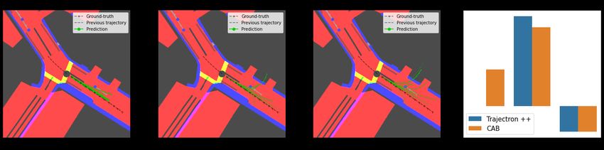
y. However, because of the very strong correlation between       Information Maximizing Categorical CVAE Trajec-
X and y in driving datasets, they tend, in practice, to learn    tron++ deviates from the standard CVAE setup in two
to focus essentially on X and to ignore C when estimating        notable ways. Firstly, following [50], they include in
p(y|X , C). In the worse cases, models can collapse into         the CVAE objective Lcvae a mutual information term
estimating simply p(y|X ). Yet, C contains crucial infor-        Iq (X , C, z) between the inputs (X , C) and the latent factor
mation such as road boundaries or pedestrians. Our goal is       z. Secondly, in Trajectron++, the latent variable z is set as
then to encourage taking C into account by introducing a         categorical. The output distribution defined in Equation 1 is
regularization term LCAB to the CVAE objective:                  then modeled as a Gaussian mixture with |Z| modes. These
                                                                 deviations are easily integrated to CAB by adding the same
                    L = Lcvae + LCAB .                    (3)    mutual information term and also setting z as categorical.
                                                                 As with Gaussian distributions that are often used in the
   The idea of LCAB is to encourage the prediction of the
                                                                 context of VAEs, the DKL between two categorical distribu-
model to be different from p (y|X ). However, in practice,
                                                                 tions has a differentiable closed-form expression.
we do not have access to this distribution. Instead, we in-
troduce a blind-mode for the CVAE model by simply re-
                                               ˜ We obtain
placing the context input C by a null context C.                 Data and implementation in Trajectron++ The dy-
           ˜ an explicitly flawed model whose predictions
pΘ (y|X , C),                                                    namic history of the agent is a multi-dimensional temporal
can then be used to steer the learning of the main model         signal X = [x–H , ..., x–1 , x0 ], where each vector xj ∈ R8
pΘ (y|X , C) away from focusing exclusively on X .               contains position, velocities, acceleration, heading and an-
   To do so, we would want LCAB to increase                      gular velocity. This sequence is encoded into a vector
                              ˜
DKL [pΘ (y|X , C)k pΘ (y|X , C)].       Unfortunately, this      x = fx (X ), where fx is designed as a recurrent neural net-
term is intractable in the general case, and computing a         work. The visual context C is represented by two quantities
robust Monte-Carlo estimate requires sampling a very large       that provide external information about the scene. The first
number of trajectories, which would significantly slow           is a bird-eye view image M ∈ {0, 1}h×w×l , constructed
down the training. Therefore, we simplify the problem by         from a high-definition map, where each element M[h, w, l]
setting this divergence constraint on the distributions over     encodes the presence or the absence of the semantic class l
z instead of the distributions over y. We thus minimize          at the position (h, w). Classes correspond to semantic types
                                                                 such as “driveable area”, “pedestrian crossing” or “walk-
                                                ˜
       LCAB-KL = −DKL [pθ (z|X , C) k pθ (z|X , C)]       (4)    way”. This tensor M is processed by a convolutional neu-
instead. Following the intuition proposed in [9], the distri-    ral network to provide m = fm (M) ∈ Rdm . The second
butions over z model intent uncertainties, whereas distribu-     quantity is a vector g ∈ Rdg that encodes the dynamic state
tions over y merge intent and control uncertainties. In this     of neighboring agents. We define the context vector c as the
                                         ˜ to have a high DKL
case, forcing pθ (z|X , C) and pθ (z|X , C)                      concatenation of m and g.
explicitly sets this constraint on high-level decisions.             As discussed here-above, distributions pθ (z|Xi , Ci ) and
   Moreover, to make sure that pΘ (y|X , C) ˜ is a reasonable    qψ (z|Xi , Ci , yi ) from Equation 2 are set as categorical dis-
approximation for p(y|X ), we also optimize parameters Θ         tributions, parameterized by the outputs of neural networks
for an additional term L̃cvae , which consists in the loss de-   fθ (x, c) and fψ (x, c, y) respectively.
scribed in Equation 2 where each Ci is replaced by C.  ˜             Then,       for each z           ∈       Z,     we have
   The final LCAB objective is then                              pφ (y|x, c, z)        =    N (µz , Σz ), where (µz , Σz ) =
                                                                 fφ (x, c, z). These Gaussian densities are weighted by
              LCAB = λKL LCAB-KL + λL̃cvae ,              (5)    the probabilities of the corresponding z, and summed to
                                                                 provide the trajectory distribution:
where λ and λKL are hyper-parameters.
   To ensure that the blind distribution focuses solely on
                                                                                         X
                                                                         pΘ (y|x, c) =         pθ (z|x, c)pφ (y|x, c, z).    (6)
approximating p(y|X ), LCAB-KL is only back-propagated                                   z∈Z
                                           ˜ We underline
along pθ (z|X , C) and not along pθ (z|X , C).
that LCAB does not introduce extra parameters.                      Interestingly, fφ is constructed as a composition of two
                                                                 functions. The first is a neural network whose output
3.3. Instanciation of CAB with Trajectron++
                                                                 is a distribution over control values for each prediction
   To show the efficiency of CAB, we use Trajectron++            timestep. The second is a dynamic integration module that
[42], a popular model for trajectory prediction based on         models temporal coherence by transforming these control
a variant of a CVAE and whose code is freely available.          distributions into 2-D position distributions. This design en-
We first discuss how the loss of Trajectron++ deviates from      sures that output trajectories are dynamically feasible. For
standard CVAE, and then present its implementation.              more details, please refer to [42].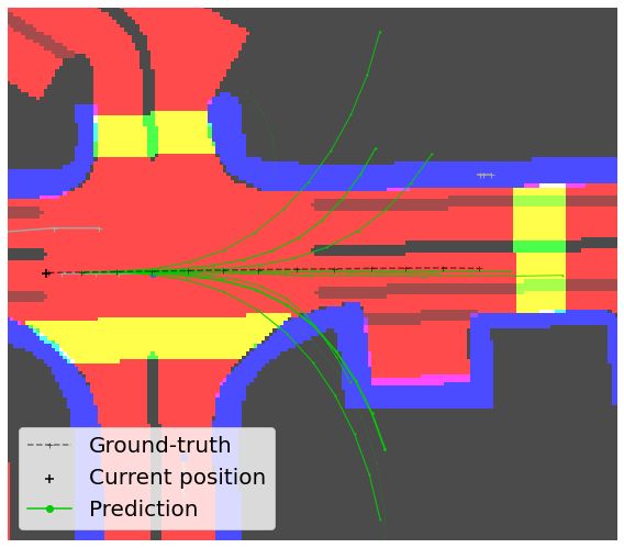
3.4. Alternative de-biasing strategies                               trained and evaluated on the official train/val/test splits from
                                                                     the nuScenes Prediction challenge, respectively containing
   We also propose two alternative de-biaising strategies.
                                                                     32186 / 8560 / 9041 instances, each corresponding to a spe-
Like CAB, they leverage blind predictions to encourage the
                                                                     cific agent at a certain time step for which we are given a
model to use the context. However, unlike CAB that plays
                                                                     2-second history (H = 4) and are expected to predict up to
on the specificity of motion forecasting by acting on distri-
                                                                     6 seconds in the future (T = 12).
bution of the latent representation, these variations are in-
spired by recent models from the VQA and NLI fields.
   • Reweight is inspired by the de-biased focal loss pro-
                                                                     4.2. Baselines and details
posed in [31]. The importance of training examples is dy-            Physics-based baselines We consider four simple physics-
namically modulated during the learning phase to focus               based models, and a Physics oracle, as introduced in [37],
more on examples poorly handled by the blind model. For-             that are purely based on motion cues and ignore contextual
mally, the model optimizes the following objective:                  elements. The four physics-based models use the current
                                                                     velocity, acceleration, and yaw rate and forecast assuming
  Lrw =Lcvae + L̃cvae
                                                                     constant speed/acceleration and yaw/yaw rate. The trajec-
         N
        X                                                (7)         tory predicted by the Physics oracle model is constructed by
       −                        ˜ log pΘ (yi |Xi , Ci ),
           σ(− log pΘ (yi |Xi , C))                                  selecting the best trajectory, in terms of average point-wise
         i=1
                                                                     Euclidean distance, from the pool of trajectories predicted
where σ represents the sigmoid function. Intuitively, sam-           by the four aforementioned physics-based models. This
ples that can be well predicted from the blind model, i.e.           Physics Oracle serves as a coarse upper bound on the best
low value of σ(− log pΘ (yi |Xi , C˜i )), will see their contribu-   achievable results from a blind model that would be purely
tion lowered and reciprocally, the ones that require contex-         based on motion dynamics and ignores the scene structure.
tual information to make accurate forecast, i.e. high value
of σ(− log pΘ (yi |Xi , C˜i )), have an increased weight. Simi-
larly to CAB, we prevent the gradients to flow back into the         Learning-based forecasting methods We compare our
blind branch from the loss weight term.                              debiased models against recently published motion predic-
    • RUBiZ adjusts gradients instead of sample impor-               tion models. CoverNet [37] forwards a rasterized represen-
tance. It does so by modulating the predictions of the main          tation of the scene and the vehicle state (velocity, accelera-
model during training to resemble more to predictions of a           tion, yaw rate) into a CNN and learns to predict the future
blind model. RUBiZ is inspired by RUBi [5], a VQA model              motion as a class, which corresponds to a pre-defined tra-
designed to mitigate language bias. Originally designed for          jectory. We re-train the “fixed  = 2” variant, for which
the classification setup, we adapt this de-biasing strategy to       the code is available, to compare it with our models. Tra-
operate over the latent factor z of our model, hence the name        jectron++ [42] is our baseline, which corresponds to re-
RUBiZ. In practice, given l and l̃ the logits of pθ (z|X , C)        moving LCAB in CAB. HalentNet [52] casts the Trajec-
               ˜ a new distribution over the latent variable
and pθ (z|X , C),                                                    tron++ model as the generator of a Generative Adversarial
is obtained as prubiz            ˜ = softmax(σ(l)∗σ(l̃)). This
                      (z|X , C, C)                                   Network (GAN) [18]. A discriminator is trained to distin-
                 θ
distribution, when used by the decoder, shifts the output            guish real trajectories from generated ones and to recognize
of the main prediction towards a blind prediction. Con-              which z was chosen to sample a trajectory. It also intro-
sequently, situations where scene information is essential           duces ‘hallucinated’ predictions in the training, which cor-
and past trajectory is not enough have increased gradient,           respond to predictions with several confounded values of
whereas easy examples that are well predicted by the blind           z. To measure the usefulness of the contextual elements
model have less importance in the global objective.                  in these models, we also consider the ‘Trajectron++ (no-
                                                                     context)’ and ‘HalentNet (no-context)’ variants that simply
4. Experiments                                                       discard the map and social interactions from the input of
                                                                     the respective underlying models. Trajectron++ and Halent-
4.1. nuScenes Dataset
                                                                     Net are not evaluated for different temporal horizons on the
   Our models are trained and evaluated on the driving               nuScenes prediction challenge splits and we thus re-train
dataset nuScenes [6]. It contains a thousand 20-second ur-           them given their respective codebases.
ban scenes recorded in Boston and Singapore. Each scene
includes data from several cameras, lidars, and radars, a
high-definition map of the scene, as well as annotations for         Implementation details We use the ADAM optimizer
surrounding agents provided at 2 Hz. These annotations are           [23], with a learning rate of 0.0003. The value of hyper-
processed to build a trajectory prediction dataset for sur-          parameters λ = 1.0 and λKL = 5.0 are found on the valida-
rounding agents, and especially for vehicles. Models are             tion set.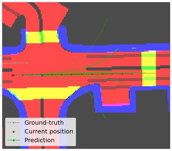
ADE-ML                                  FDE-ML                    OffR-ML ADE-f FDE-f OffR-f
                   Model    @1s    @2s    @3s @4s     @5s    @6s    @1s    @2s    @3s @4s     @5s    @6s       @6s    @6s   @6s   @6s
    Constant vel. and yaw   0.46   0.94   1.61 2.44   3.45   4.61   0.64   1.74   3.37 5.53   8.16   11.21     0.14     -     -     -
          Physics Oracle    0.43   0.82   1.33 1.98   2.76   3.70   0.59   1.45   2.69 4.35   6.47    9.09     0.12     -     -     -
    Covernet, fixed  = 2   0.81   1.41   2.11 2.93   3.88   4.93   1.07   2.35   3.92 5.90   8.30   10.84     0.11     -     -     -
Trajectron++ (no-context)   0.13   0.39   0.87 1.59   2.56   3.80   0.15   0.86   2.23 4.32   7.22   10.94     0.27   4.46 12.32  0.36
            Trajectron++    0.13   0.39   0.86 1.55   2.47   3.65   0.15   0.87   2.16 4.15   6.92   10.45     0.23   4.15 11.44  0.29
   HalentNet (no-context)   0.12   0.38   0.82 1.43   2.21   3.17   0.13   0.85   2.04 3.72   5.92    8.64     0.27   4.13 10.95  0.29
               HalentNet    0.14   0.41   0.87 1.51   2.32   3.29   0.17   0.88   2.14 3.91   6.15    8.83     0.28   3.98 10.61  0.25
                Reweight    0.13   0.38   0.81 1.42   2.20   3.14   0.15   0.83   2.00 3.69   5.90    8.58     0.17   3.71  9.74  0.19
                   RUBiZ    0.18   0.42   0.82 1.40   2.14   3.04   0.23   0.84   1.95 3.55   5.65    8.21     0.11   3.68  9.45  0.17
                     CAB    0.12   0.34   0.73 1.29   2.01   2.90   0.14   0.73   1.81 3.39   5.47    8.02     0.13   3.41  9.03  0.20

Table 1. Trajectory forecasting on the nuScenes Prediction challenge [6]. Reported metrics are the Average/Final Displacement Error
(ADE/FDE), and the Off-road Rate (OffR). Each metric is computed for both the most-likely trajectory (-ML) and the full distribution (-f ).

4.3. Results and standard evaluations                                      the forecasting abilities of purely motion-based models and
                                                                           we observe that learning-based methods hardly outperform
    We compare our debiased models to the baselines by                     this Physics-oracle on long temporal horizons.
measuring the widely used metrics of displacement and off-
                                                                              On the other hand, we remark that all three of our de-
road rate. All models are trained to predict 6 seconds in the
                                                                           biaising strategies significantly outperform the Physics or-
future, and their performance is evaluated for varying tem-
                                                                           acle and previous models on almost all the metrics, both
poral horizons (T ∈ {2, 4, 6, 8, 10, 12}). Average Displace-
                                                                           when looking at the most-likely trajectory as well as the full
ment Error (ADE) and Final Displacement Error (FDE)
                                                                           future distribution. This validates the idea, shared in our
measure the distance between the predicted and the ground-
                                                                           methods, to enforce the model’s prediction to have a high
truth trajectory, either as an average between each corre-
                                                                           divergence with a blind prediction. Indeed, despite opti-
sponding pair of points (ADE), or as the distance between
                                                                           mizing very different objective functions, our Reweight and
final points (FDE). To compute these metrics with CAB, we
                                                                           RUBiZ and CAB share the idea of a motion-only encoding.
sample the most likely trajectory yML by first selecting the
                                                                           More precisely, at a 6-second horizon, the sample reweight-
most likely latent factor zML = arg maxz∈Z pθ (z|x, c), and
                                                                           ing strategy gives a relative improvement of 16% w.r.t. Tra-
then computing the mode of the corresponding Gaussian
                                                                           jectron++. The more refined RUBiZ strategy of gradient
yML = arg maxy pφ (y|x, c, zML ). To evaluate the quality
                                                                           reweighting gives a relative improvement of 19% w.r.t. Tra-
of the whole distribution and not just the most-likely tra-
                                                                           jectron++. CAB achieves a 22% relative improvement over
jectory, similarly to [42, 52], we compute metrics ‘ADE-f’
                                                                           Trajectron++. This indicates that guiding the model’s latent
and ‘FDE-f’. They are respectively the average and final
                                                                           variable constitutes a better use of blind predictions than
displacement error averaged for 2000 trajectories randomly
                                                                           simple example or gradient weightings.
sampled in the full distribution predicted by the network
yfull ∼ pΘ (y|x, c). Finally, the ‘off-road rate’ (OffR) is the
                                                                           4.4. Further analyses: stability, convergence, Shap-
rate of future trajectories that leave the driveable area.
                                                                                 ley values
    In Table 1, we compare the performance of our mod-
els CAB, Reweight and RUBiZ with baselines from the                            We hypothesize that properly leveraging contextual in-
recent literature. To begin with, we remark that for the                   formation has a strong impact on the ability to anticipate
Trajectron++ model, the use of context brings close to no                  the agent’s intents. Intuitively, for an agent arriving at an
improvement for predictions up to 4 seconds and a very                     intersection, a model without context will begin predicting
small one for 5- and 6-second horizons. Even more sur-                     a stopping trajectory only from the moment when this agent
prisingly, the HalentNet (no-context) model which does not                 starts to stop, whereas a model with a proper understanding
use any information from the surroundings, shows better                    of contextual information will be able to foresee this be-
ADE-ML and FDE-ML than the regular context-aware Ha-                       havior change ahead in time. Furthermore, improving this
lentNet model. This supports our claim that the contextual                 anticipation ability should also help the temporal stability
elements are overlooked by these models and that predic-                   of the predictions, as unanticipated changes of trajectory
tions are mostly done by relying on motion cues. Moreover,                 will be less likely. Unfortunately, ADE and FDE metrics
we emphasize that the Physics oracle — which is purely                     do not explicitly measure the rate of convergence towards
based on motion dynamics — obtains very strong perfor-                     the ground-truth, nor the stability of successive predictions.
mances (3.70 ADE-ML@6s, 9.09 FDE-ML@6s) as it can                              Consequently, we introduce two new metrics focusing
choose the closest trajectory to the ground truth from a va-               on the stability and convergence rate of successive fore-
riety of dynamics. Its scores approximate upper bounds on                  casts. Instead of classically looking at the T -step forecast
Figure 3. Visualizations of predicted trajectories and Shapley values. The thickness of lines represent the probability of each trajectory.
Dispersion D ↓
Convergence-to-range C(τ ) ↑ ter of {ytt̂−t }t∈J1,T K . The global dispersion score D is ob-
Model τ = 20cm τ = 1m τ = 5m
Cst. accel., yaw 6.55 0.44 1.49 3.30
tained by averaging these values over all the points in the
Cst. accel., yaw rate 6.03 0.47 1.58 3.46 dataset. Moreover, we propose the convergence-to-range-τ
Cst. speed, yaw rate 3.42 0.54 1.82 4.15 metric C(τ )t̂ as the time from which all subsequent predic-
Cst. vel., yaw 3.33 0.53 1.82 4.16
Physics Oracle 2.99 0.55 1.91 4.38
tions fall within a margin τ of the ground-truth yt̂gt , where τ
Covernet, fixed = 2 4.06 0.15 0.93 3.50 is a user-defined threshold:
Trajectron++ (no-context) 3.65 1.00 2.11 4.17
Trajectron++ 3.55 0.98 2.11 4.22
Ct̂ (τ ) = max T 0 ∈ J1, T K | ∀t ≤ T 0 , kytt̂−t −yt̂gt k2 ≤ τ .
Halentnet (no-context) 2.85 1.03 2.28 4.59
Halentnet 3.23 0.90 2.07 4.26 (8)
Reweight 3.02 1.03 2.27 4.50
RUBiZ 2.73 0.94 2.31 4.60
In Table 2, we report evaluations of the stability and spa-
CAB 2.61 1.12 2.45 4.74 tial convergence metrics. First, we observe that previous
learning-based forecasting models have more limited antic-
Table 2. Study of the temporal stability of trajectory predic- ipation capacities than the simpler physics-based models,
tion, with the Dispersion (D) and Convergence-to-range (C(τ )) in terms of both convergence speed (metric C(τ )) and con-
metrics. Predictions are made at a 6-second horizon.
vergence stability (metric D). Consistently to the results
of Table 1, we remark that our de-biased strategies, and es-
pecially our main model CAB, lead to better anticipation
yt = [y1t , . . . , yTt ] made at a specific time t, we take a
scores as they converge faster towards the ground truth.
dual viewpoint by considering the consecutive predictions
In Figure 3, we visualize trajectories generated by
[yTt̂−T , . . . , y1t̂−1 ] made for the same ground-truth point yt̂gt .
CAB and the baselines Trajectron++ and Trajectron++ (no-
When the agent approaches the timestamp t̂, as t grows, context). We also analyze the contribution brought by each
predictions ytt̂−t will get closer to the ground-truth yt̂gt . In input of the model. To do so, we estimate the Shapley val-
addition to low ADE/FDE scores, it is desirable to have ues [28] which correspond to the signed contribution of in-
both (1) a high consistency of consecutive predictions, as dividual input features on a scalar output, the distance to the
well as (2) a fast convergence towards the ground-truth final predicted point in our case. We remark that the Shap-
yt̂gt . Therefore, for a given annotated point at t̂, we define ley value of the state signal is overwhelmingly higher than
the dispersion Dt̂ as the standard deviation of the points the ones attributed to the map and the neighbors for Tra-
predicted by the model for this specific ground-truth point jectron++. This means that the decisions are largely made
Dt̂ = STD ( kytt̂−t − ȳt̂ k)t∈J1,T K where ȳt̂ is the barycen- from the agent’s dynamics. This can further be seen as sev-Model 1% 2% 3% All
Trajectron++ (no-context) 15.80 15.58 14.97 10.94
Trajectron ++ 13.12 12.69 12.25 10.45
HalentNet 14.12 12.83 12.09 8.83
Reweight 14.00 13.30 12.58 8.58
RUBiZ 13.42 12.49 11.64 8.21
CAB 12.13 11.88 11.59 8.02
Table 3. Final Displacement Error FDE@6s on challenging
situations, as defined by Makansi et al. [32]. Results for columns
‘i%’ are averaged over the top i% hardest situations as measured
by the the mismatch between the prediction from a Kalman filter
and the ground-truth.
eral predicted trajectories are highly unlikely futures as they
collide with the other agents and/or leave the driveable area.
Instead, the Shapley values for CAB give much more im-
portance to both the map and the neighboring agents, which
helps to generate likely and acceptable futures.
4.5. Evaluation on hard situations
We verify that the performance boost observed in Ta-
ble 1 does not come at the expense of a performance drop
on difficult yet critical situations. Accordingly, we use re-
cently proposed evaluations [32] as they remark that uncrit-
ical cases dominate the prediction and that complex scenar-
ios cases are at the long tail of the dataset distribution. In
practice, situations are ranked based on how well the fore-
cast made by a Kalman filter fits the ground-truth trajectory.
In Table 3, we report such stratified evaluations, on the Figure 4. Visualizations on challenging situations, as defined
1%, 2%, and 3% hardest situations. Our first observation by Makansi et al. [32]. By better leveraging the context, CAB
is that the overall performance (‘All’) does not necessar- generates more accurate predictions while Trajectron++ leaves the
ily correlate with the capacity to anticipate hard situations. driveable area or collides into other agents.
Indeed, while HalentNet significantly outperfoms Trajec-
tron++ on average, it falls short on the most challenging 5. Conclusion
cases. Besides, CAB achieves better results than Trajec- We showed that modern motion forecasting models
tron++ on the hardest situations (top 1%, 2%, and 3%). struggle to use contextual scene information. To address
Lastly, while the gap between Trajectron++ and CAB is this, we introduced blind predictions that we leveraged with
only 0.66 point for the 3% of hard examples, it increases novel de-biaising strategies. This results into three mo-
for the top 1% of hardest examples up to 0.99. tion forecasting models designed to focus more on con-
In Figure 4, we display some qualitative results we ob- text. We show that doing so helps reducing statistical biases
tain on challenging situations selected among the 1% hard- from which learning-based approaches suffer. In particular,
est examples. On the left, we observe that the turn is not CAB, which is specifically built for probabilistic forecast-
correctly predicted by Trajectron++ as it estimates several ing models, makes significant improvements in traditional
possible futures that leave the driveable area. On the right, distance-based metrics. Finally, after introducing new sta-
the agent of interest has to stop because of stopped agents in bility and convergence metrics, we show that CAB shows
front of it and this behavior is well forecasted by CAB, un- better anticipation properties than concurrent methods.
like Trajectron++ which extrapolates the past and provides Acknowledgments: We thank Thibault Buhet, Auguste
multiple futures colliding into other agents. Overall, the Lehuger and Ivan Novikov for insightful comments. This
better use of the context in CAB not only helps on average work was supported by ANR grant VISA DEEP (ANR-20-
situations but also on difficult and potentially critical ones. CHIA-0022) and MultiTrans (ANR-21-CE23-0032).References vehicle longitudinal control with forward camera. CoRR,
abs/1812.05841, 2018. 1, 3
[1] Aishwarya Agrawal, Dhruv Batra, and Devi Parikh. Ana-
[16] Thomas Gilles, Stefano Sabatini, Dzmitry Tsishkou, Bog-
lyzing the behavior of visual question answering models. In
dan Stanciulescu, and Fabien Moutarde. GOHOME: graph-
EMNLP, 2016. 3
oriented heatmap output for future motion estimation. CoRR,
[2] Aishwarya Agrawal, Dhruv Batra, Devi Parikh, and Anirud- abs/2109.01827, 2021. 2
dha Kembhavi. Don’t just assume; look and answer: Over- [17] Thomas Gilles, Stefano Sabatini, Dzmitry Tsishkou, Bogdan
coming priors for visual question answering. In CVPR, 2018. Stanciulescu, and Fabien Moutarde. HOME: heatmap output
3 for future motion estimation. In IITSC, 2021. 2
[3] Mayank Bansal, Alex Krizhevsky, and Abhijit S. Ogale. [18] Ian J. Goodfellow, Jean Pouget-Abadie, Mehdi Mirza, Bing
Chauffeurnet: Learning to drive by imitating the best and Xu, David Warde-Farley, Sherjil Ozair, Aaron C. Courville,
synthesizing the worst. In Robotics: Science and Systems and Yoshua Bengio. Generative adversarial nets. In NIPS,
XV, 2019. 1, 2 2014. 2, 5
[4] Thibault Buhet, Émilie Wirbel, and Xavier Perrotton. PLOP: [19] Agrim Gupta, Justin Johnson, Li Fei-Fei, Silvio Savarese,
probabilistic polynomial objects trajectory planning for au- and Alexandre Alahi. Social GAN: socially acceptable tra-
tonomous driving. In CoRL, Proceedings of Machine Learn- jectories with generative adversarial networks. In CVPR,
ing Research, 2020. 1 2018. 2
[5] Rémi Cadène, Corentin Dancette, Hedi Ben-younes, [20] Joey Hong, Benjamin Sapp, and James Philbin. Rules of the
Matthieu Cord, and Devi Parikh. Rubi: Reducing unimodal road: Predicting driving behavior with a convolutional model
biases for visual question answering. In NeurIPS, 2019. 2, of semantic interactions. In CVPR, 2019. 2
3, 5 [21] Boris Ivanovic and Marco Pavone. The trajectron: Proba-
[6] Holger Caesar, Varun Bankiti, Alex H. Lang, Sourabh Vora, bilistic multi-agent trajectory modeling with dynamic spa-
Venice Erin Liong, Qiang Xu, Anush Krishnan, Yu Pan, Gi- tiotemporal graphs. In ICCV, 2019. 1, 2, 3
ancarlo Baldan, and Oscar Beijbom. nuscenes: A multi- [22] Byeoungdo Kim, Chang Mook Kang, Jaekyum Kim, Seung-
modal dataset for autonomous driving. In CVPR, 2020. 1, 2, Hi Lee, Chung Choo Chung, and Jun Won Choi. Probabilis-
5, 6 tic vehicle trajectory prediction over occupancy grid map via
[7] Sergio Casas, Cole Gulino, Renjie Liao, and Raquel Urta- recurrent neural network. In ITSC, 2017. 1
sun. Spagnn: Spatially-aware graph neural networks for rela- [23] Diederik P. Kingma and Jimmy Ba. Adam: A method for
tional behavior forecasting from sensor data. In ICRA, 2020. stochastic optimization. In ICLR, 2015. 5
1, 2 [24] Kris M. Kitani, Brian D. Ziebart, James Andrew Bagnell,
[8] Sergio Casas, Wenjie Luo, and Raquel Urtasun. Intentnet: and Martial Hebert. Activity forecasting. In ECCV, 2012. 2
Learning to predict intention from raw sensor data. In CoRL, [25] Yann LeCun, Urs Muller, Jan Ben, Eric Cosatto, and Beat
2018. 1, 2 Flepp. Off-road obstacle avoidance through end-to-end
[9] Yuning Chai, Benjamin Sapp, Mayank Bansal, and Dragomir learning. In NIPS, 2005. 1, 3
Anguelov. Multipath: Multiple probabilistic anchor trajec- [26] Namhoon Lee, Wongun Choi, Paul Vernaza, Christopher B.
tory hypotheses for behavior prediction. In CoRL, Proceed- Choy, Philip H. S. Torr, and Manmohan Chandraker. DE-
ings of Machine Learning Research, 2019. 1, 2, 4 SIRE: distant future prediction in dynamic scenes with inter-
[10] Ming-Fang Chang, John Lambert, Patsorn Sangkloy, Jag- acting agents. In CVPR, 2017. 2, 3
jeet Singh, Slawomir Bak, Andrew Hartnett, De Wang, Peter [27] Stéphanie Lefèvre, Dizan Vasquez, and Christian Laugier. A
Carr, Simon Lucey, Deva Ramanan, and James Hays. Argo- survey on motion prediction and risk assessment for intelli-
verse: 3d tracking and forecasting with rich maps. In CVPR, gent vehicles. ROBOMECH journal, 2014. 1
2019. 1 [28] Scott M. Lundberg and Su-In Lee. A unified approach to
[11] Felipe Codevilla, Eder Santana, Antonio M. López, and interpreting model predictions. In NIPS, 2017. 7
Adrien Gaidon. Exploring the limitations of behavior [29] Wenjie Luo, Bin Yang, and Raquel Urtasun. Fast and furi-
cloning for autonomous driving. In ICCV, 2019. 1, 3 ous: Real time end-to-end 3d detection, tracking and motion
[12] Henggang Cui, Vladan Radosavljevic, Fang-Chieh Chou, forecasting with a single convolutional net. In CVPR, 2018.
Tsung-Han Lin, Thi Nguyen, Tzu-Kuo Huang, Jeff Schnei- 1, 2
der, and Nemanja Djuric. Multimodal trajectory predictions [30] Yuexin Ma, Xinge Zhu, Sibo Zhang, Ruigang Yang, Wen-
for autonomous driving using deep convolutional networks. ping Wang, and Dinesh Manocha. Trafficpredict: Trajectory
In ICRA, 2019. 1, 2 prediction for heterogeneous traffic-agents. In AAAI, 2019.
[13] Pim de Haan, Dinesh Jayaraman, and Sergey Levine. Causal 2
confusion in imitation learning. In NeurIPS, 2019. 3 [31] Rabeeh Karimi Mahabadi, Yonatan Belinkov, and James
[14] Nachiket Deo and Mohan M. Trivedi. Convolutional social Henderson. End-to-end bias mitigation by modelling biases
pooling for vehicle trajectory prediction. In CVPR Work- in corpora. In ACL, 2020. 2, 3, 5
shops, 2018. 2 [32] Osama Makansi, Özgün Çiçek, Yassine Marrakchi, and
[15] Laurent George, Thibault Buhet, Émilie Wirbel, Gaetan Le- Thomas Brox. On exposing the challenging long tail in fu-
Gall, and Xavier Perrotton. Imitation learning for end to end ture prediction of traffic actors. In ICCV, 2021. 8[33] Osama Makansi, Julius Von Kügelgen, Francesco Locatello, [43] Maximilian Schäfer, Kun Zhao, Markus Bühren, and Anton
Peter Vincent Gehler, Dominik Janzing, Thomas Brox, and Kummert. Context-aware scene prediction network (casp-
Bernhard Schölkopf. You mostly walk alone: Analyzing fea- net). CoRR, abs/2201.06933, 2022. 2
ture attribution in trajectory prediction. In ICLR, 2022. 1
[44] Kihyuk Sohn, Honglak Lee, and Xinchen Yan. Learning
[34] Varun Manjunatha, Nirat Saini, and Larry S. Davis. Ex- structured output representation using deep conditional gen-
plicit bias discovery in visual question answering models. In erative models. In NIPS, 2015. 2
CVPR, 2019. 3
[35] Kaouther Messaoud, Nachiket Deo, Mohan M. Trivedi, and [45] Shashank Srikanth, Junaid Ahmed Ansari, Karnik Ram R.,
Fawzi Nashashibi. Multi-head attention with joint agent-map Sarthak Sharma, J. Krishna Murthy, and K. Madhava Kr-
representation for trajectory prediction in autonomous driv- ishna. INFER: intermediate representations for future pre-
ing. CoRR, abs/2005.02545, 2020. 1, 2 diction. In IROS, 2019. 2
[36] Gregory P. Meyer, Jake Charland, Shreyash Pandey, Ankit [46] Yichuan Charlie Tang and Ruslan Salakhutdinov. Multiple
Laddha, Shivam Gautam, Carlos Vallespi-Gonzalez, and futures prediction. In NeurIPS, 2019. 2, 3
Carl K. Wellington. Laserflow: Efficient and probabilistic
object detection and motion forecasting. IEEE Robotics Au- [47] Éloi Zablocki, Hedi Ben-Younes, Patrick Pérez, and
tom. Lett., 2021. 1, 2 Matthieu Cord. Explainability of vision-based au-
tonomous driving systems: Review and challenges. CoRR,
[37] Tung Phan-Minh, Elena Corina Grigore, Freddy A. Boulton,
abs/2101.05307, 2021. 1
Oscar Beijbom, and Eric M. Wolff. Covernet: Multimodal
behavior prediction using trajectory sets. In CVPR, 2020. 1, [48] John R. Zech, Marcus A. Badgeley, Manway Liu, An-
2, 5 thony B. Costa, Joseph J. Titano, and Eric K. Oermann.
[38] Sainandan Ramakrishnan, Aishwarya Agrawal, and Stefan Confounding variables can degrade generalization perfor-
Lee. Overcoming language priors in visual question answer- mance of radiological deep learning models. CoRR,
ing with adversarial regularization. In NeurIPS, 2018. 3 abs/1807.00431, 2018. 3
[39] Nicholas Rhinehart, Kris M. Kitani, and Paul Vernaza. r2p2: [49] Wenyuan Zeng, Wenjie Luo, Simon Suo, Abbas Sadat, Bin
A reparameterized pushforward policy for diverse, precise Yang, Sergio Casas, and Raquel Urtasun. End-to-end inter-
generative path forecasting. In ECCV, 2018. 2 pretable neural motion planner. In CVPR, 2019. 1, 2
[40] Nicholas Rhinehart, Rowan McAllister, Kris Kitani, and [50] Shengjia Zhao, Jiaming Song, and Stefano Ermon. Info-
Sergey Levine. PRECOG: prediction conditioned on goals vae: Balancing learning and inference in variational autoen-
in visual multi-agent settings. In ICCV, 2019. 2, 3 coders. In AAAI, 2019. 4
[41] Amir Sadeghian, Vineet Kosaraju, Ali Sadeghian, Noriaki
Hirose, Hamid Rezatofighi, and Silvio Savarese. Sophie: An [51] Tianyang Zhao, Yifei Xu, Mathew Monfort, Wongun Choi,
attentive GAN for predicting paths compliant to social and Chris L. Baker, Yibiao Zhao, Yizhou Wang, and Ying Nian
physical constraints. In CVPR, 2019. 2 Wu. Multi-agent tensor fusion for contextual trajectory pre-
diction. In CVPR, 2019. 2
[42] Tim Salzmann, Boris Ivanovic, Punarjay Chakravarty, and
Marco Pavone. Trajectron++: Dynamically-feasible trajec- [52] Deyao Zhu, Mohamed Zahran, Li Erran Li, and Mohamed
tory forecasting with heterogeneous data. In ECCV, 2020. 1, Elhoseiny. Halentnet: Multimodal trajectory forecasting
2, 3, 4, 5, 6 with hallucinative intents. In ICLR, 2021. 2, 3, 5, 6You can also read