Quantum Face Recognition Protocol with Ghost Imaging
←
→
Page content transcription
If your browser does not render page correctly, please read the page content below
Quantum Face Recognition Protocol with Ghost Imaging

                                                                 Vahid Salari,1, 2, ∗ Dilip Paneru,3 Erhan Saglamyurek,4, 5 Milad Ghadimi,6 Moloud Abdar,7
                                                                  Mohammadreza Rezaee,3 Mehdi Aslani,6 Shabir Barzanjeh,5 and Ebrahim Karimi3, 8, †
                                                        1
                                                         BCAM - Basque Center for Applied Mathematics; Alameda de Mazarredo, 14,48009 Bilbao, Basque Country - Spain
                                                                            2
                                                                              Department of Physics and Astronomy, Howard University, Washington DC, USA
                                                   3
                                                     Department of physics, University of Ottawa, Advanced Research Complex, 25 Templeton Street, K1N 6N5, Ottawa, ON, Canada
                                                                             4
                                                                               Department of Physics, University of Alberta, Edmonton, AB T6G 2E1, Canada
                                                                    5
                                                                      Department of Physics and Astronomy, University of Calgary, Calgary, AB T2N 1N4 Canada
                                                                          6
                                                                            Department of Physics, Isfahan University of Technology, Isfahan 8415683111, Iran
                                                                    7
                                                                      Institute for Intelligent Systems Research and Innovation (IISRI), Deakin University, Australia
                                                                       8
                                                                         National Research Council of Canada, 100 Sussex Drive, K1A 0R6, Ottawa, ON, Canada
                                                                                                         (Dated: October 20, 2021)
arXiv:2110.10088v1 [quant-ph] 19 Oct 2021

                                                             Face recognition is one of the most ubiquitous examples of pattern recognition in machine learning, with
                                                             numerous applications in security, access control, and law enforcement, among many others. Pattern
                                                             recognition with classical algorithms requires significant computational resources, especially when deal-
                                                             ing with high-resolution images in an extensive database. Quantum algorithms have been shown to im-
                                                             prove the efficiency and speed of many computational tasks, and as such, they could also potentially
                                                             improve the complexity of the face recognition process. Here, we propose a quantum machine learning
                                                             algorithm for pattern recognition based on quantum principal component analysis (QPCA), and quan-
                                                             tum independent component analysis (QICA). A novel quantum algorithm for finding dissimilarity in
                                                             the faces based on the computation of trace and determinant of a matrix (image) is also proposed. The
                                                             overall complexity of our pattern recognition algorithm is O(N log N ) – N is the image dimension. As an
                                                             input to these pattern recognition algorithms, we consider experimental images obtained from quantum
                                                             imaging techniques with correlated photons, e.g. “interaction-free” imaging or “ghost” imaging. Inter-
                                                             facing these imaging techniques with our quantum pattern recognition processor provides input images
                                                             that possess a better signal-to-noise ratio, lower exposures, and higher resolution, thus speeding up the
                                                             machine learning process further. Our fully quantum pattern recognition system with quantum algo-
                                                             rithm and quantum inputs promises a much-improved image acquisition and identification system with
                                                             potential applications extending beyond face recognition, e.g., in medical imaging for diagnosing sensitive
                                                             tissues or biology for protein identification.

                                                                      INTRODUCTION                                     As a second important step, pattern recognition in the ac-
                                                                                                                    quired images is a prominent feature of any intelligent imag-
                                               In any intelligent image processing system, there are es-            ing system. Face recognition [4] is one of the branches of
                                            sentially two main steps: the acquisition of the image and              pattern recognition, with numerous applications such as face
                                            the recognition of the desired patterns. Image acquisition for          ID verification, passport checks, entrance control, computer
                                            any pattern recognition method can be performed in multiple             access control, criminal investigations, crowd surveillance,
                                            ways. For instance, classical sources (incoherent light from            and witness face reconstruction [5], among several others.
                                            thermal radiation or a coherent beam from a laser) or quantum           For face recognition, several classical machine learning algo-
                                            sources (entangled photons obtained from down conversion                rithms exist [6], generally requiring huge computational re-
                                            or squeezed light) can be used to obtain the images. Clas-              sources especially when faced with the problem of identifi-
                                            sical bright field imaging techniques employing the former              cation from a large database. Quantum machine learning al-
                                            sources, have the disadvantage of high probe illumination re-           gorithms employing quantum features such as superposition
                                            quirement, especially while imaging sensitive samples. Ad-              and entanglement [7–15] promise enhancements in terms of
                                            ditionally, they are also plagued by the shot noise inherent in         the computing resources and the speed compared to the clas-
                                            the intensities, and the background noise from the environ-             sical counterparts. Several experimental researches have been
                                            ment. Quantum techniques such as quantum illumination, or               done to implement these algorithms [16–21]. In this article,
                                            ghost imaging or even interaction-free imaging, alleviates the          we present a quantum algorithm for face recognition as one of
                                            problems of background noise, and the probe illumination by             the potential applications of quantum algorithms in machine
                                            utilizing quantum correlations between photon pairs [1]. Fur-           learning.
                                            thermore, quantum sub-shot noise imaging [2] and super res-                The problem of identification of faces from any images gen-
                                            olution techniques [3] enhance the noise sensitivity and reso-          erally constitutes different steps (shown in Figure 1): cre-
                                            lution in any images beyond the classical limits.                       ating a database of faces consisting of training and test im-
                                                                                                                    ages, feature extraction using principal component analysis
                                                                                                                    (PCA), linear discriminant analysis (LDA) or independent
                                                                                                                    component analysis (ICA), feature matching using dissimilar-
                                            ∗   vsalari@bcamath.org                                                 ity measures, and recognition [22]. PCA extracts the eigen-
                                            †   ekarimi@uottawa.ca                                                  states (or eigenfaces) of the covariance matrix of the images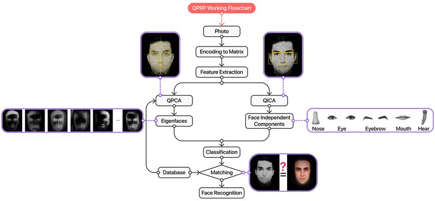
2

FIG. 1. Flowchart of the quantum algorithm for face recognition. The quantum algorithm is proposed to be performed in a quantum
processor, which we call it quantum pattern recognition processor (QPRP). First the image is converted into matrix form, on which feature
extraction algorithms such as quantum principal component analysis (QPCA) or quantum independent component analysis (QICA) are applied.
QPCA extracts the eigenstates (or eigenfaces) of the covariance matrix of the images in the database. The eigenfaces include information like
average face, gender (male, female), face direction, brightness, shadows, etc. QICA extracts the independent elements such as eyes, eyebrows,
mouth, nose, etc. in a face. The complexity of this stage is O(log N ) – N is the dimension of th image. Then, the given faces are compared
with the faces in the database by using dissimilarity measure based on the log determinant divergence, and the best match among the faces in
the database is identified.

in the database, including information like average face, gen-          dits) to classical data (bits), most of the information is lost in
der (male or female), face direction, brightness, shadows, etc.         the measurement process, due to the “collapse” of the wave-
ICA, however, extracts the independent elements such as eyes,           function. Although techniques such as quantum state tomog-
eyebrows, mouth, nose, etc. in a face. Quantum algorithms               raphy implemented on unlimited ensemble of the states can
which provide speedup for PCA and ICA have already been                 be used to fully reconstruct the quantum states from classical
proposed [7, 23]. Here, we focus on three main steps: (1)               projections, these processes are generally complex and expen-
Quantum Principle Component Analysis (QPCA) [7], (2)                    sive. Therefore, the optimal input to our quantum algorithms,
Quantum Independent Component Analysis (QICA) [23], and                 would be the quantum states directly obtained from quantum
(3) Dissimilarity measures (i.e., face matching), to develop            processes, for example, quantum imaging methods, or from a
a quantum algorithm for face recognition. In what follows,              quantum memory, without performing a strong measurement
we present a quantum algorithm for dissimilarity measures for           on the wavefunction.
face matching with speedup. This is based on a quantum al-
gorithm to compute the log determinant divergence using both               Photonic quantum memories [24], allowing storage and
the determinant and the trace of a matrix. Our algorithm com-           on-demand retrieval of quantum states of light, is one of
bined with the inputs obtained from quantum imaging tech-               the key components for the realization of quantum optical
niques provides a fully intelligent pattern identification sys-         pattern-recognition technology. Quantum memories essen-
tem, with the joint benefit of the low-dose and higher res-             tially form a quantum database for the matching stage in the
olution of quantum imaging methods, and the speedup and                 recognition process. With the state-of-art quantum memories,
efficiency of the quantum algorithms. Figure 1 shows the                the possibility of storing hundreds of spatial modes has al-
flowchart of the quantum algorithm for the pattern identifi-            ready been shown in experimental studies using atomic-cold
cation.                                                                 gases [25, 26]. Furthermore, using solid-state atomic mem-
                                                                        ories, it is possible to simultaneously store hundreds of pho-
                                                                        tonic quantum states in distinct temporal modes, thus allow-
                                                                        ing us to store patterns scanned at separate times [27, 28]. In
              QUANTUM FACE RECOGNITION                                  addition, optically accessible spin-states of certain atomic sys-
                                                                        tems can reach several hours of coherence time [29]. A very
   Classical algorithms are unable to process quantum data              recent experimental demonstration reports one-hour memory
directly. During the conversion of the quantum states (qu-              lifetime for light storage, showing the feasibility of long-lived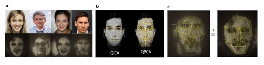
3

FIG. 2. Intelligent pattern recognition in quantum imaging. Data from quantum imaging methods such as (a) Interaction Free Imaging
and (b) Ghost Imaging act as an input to (c) Quantum Pattern Recognition Processor (QPRP). The latter, i.e., QPRP, applies quantum machine
learning to find the patterns in the database.

photonic quantum memory devices [30]. Atomic memory ap-                ton Avalanche Diode (SPAD) detector – see Supplementary
proaches have also been shown to reach high retrieval effi-            Information (SI) for the detail of the experimental setup.
ciencies up to 92% [31] and high fidelities above 99% [32].
However, an implementation with all of the aforementioned
properties still remains as a challenge in developing a practi-              A.    Quantum principal component analysis (QPCA)
cal quantum database memory.
                                                                          We have now the input images either retrieved from a quan-
   Quantum techniques such as quantum ghost imaging [33],
                                                                       tum memory or directly as outputs from a quantum imaging
quantum lithography [34], or quantum sensing [35], when
                                                                       setup. The pattern recognition processor applies Quantum
appropriately interfaced with photonic quantum processors,
                                                                       Principal Component Analysis (QPCA) [7, 38] to extract the
for example an array of optical fibers connected to an inte-
                                                                       principal eigenvectors of the covariance matrix CX , formed
grated quantum photonic circuit, can also act as inputs to our
                                                                       by the set of the training images.
algorithms (see Figure 2). Here for the case of our face
                                                                          Let us consider a set of N -dimensional training images (or
recognition algorithm, we assume that the input images are
                                                                       faces), {|x(1) i, . . . , |x(M ) i}. Here, |x(i) i is the i-th training
acquired by quantum ghost imaging [33]. Ghost imaging
                                                                       image, which is given by,
exploits the spatial correlations between photon pairs gener-
ated through a nonlinear process called spontaneous paramet-                                             N
                                                                                                         X
ric down-conversion (SPDC). Since the images are obtained                                    |x(i) i =         xq(i) |ψq(i) i,            (1)
by triggering the shutter in order to capture only the “coinci-                                          q=1
dent” photon pairs, the level of background noise is signifi-                     (i)                                    (i)
cantly reduced, along with a reduction in probe illumination.          where xq are the components, and |ψq i are the basis kets.
In a variation of this technique using non degenerate photon           The covariance matrix CX can be formed as a sum over M
pairs, the image detection and sample interaction can happen           training faces [38],
at different wavelengths, which can be useful when imaging                                            M
                                                                                                   1 X (i) (i)
sensitive tissues when limited in detection technologies [36].                             CX =          |x ihx |.                        (2)
Combining quantum detection techniques such as interaction-                                        M i=1
free measurement with ghost imaging, the illumination level            The next step is to exponentiate the covariance matrix CX ,
required for the same levels of Signal to Noise ratio (SNR) in         so that we can use the Quantum Phase Estimation (QPE)
images [37] is further reduced significantly. Figure 3 shows           subroutine for finding the eigenvectors and eigenvalues. It has
some of the images of human faces obtained in a quantum                been shown that the exponentiation of the covariance matrix,
ghost imaging setup, where spatially correlated photon pairs           i.e., e−iCX t , can be performed in O(log N ) time [7].
(namely signal and idler), are generated by pumping a BiBO
crystal with pump photons. Phase holograms placed in a Spa-               In QPCA algorithm, for the phase estimation subroutine,
tial Light Modulator, a liquid crystal device, created by super-       we apply the operator U = e−iCX t on CX [38]. The action
imposing the human faces with a diffraction grating acts as an         of U on one of the states |x(i) i in CX is:
object for the signal photon, while the idler photon passes to
                                                                                                               M
the Intensified Charged Coupled Devices (ICCD) camera via                                                      X
a delay line. The images are obtained by triggering the ICCD                            e−iCX t |x(i) i →            c(ij) |φj i,         (3)
shutter with the signal photons detected through a Single Pho-                                                 j=1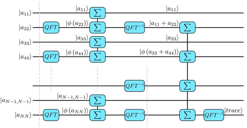
4

FIG. 3. Face recognition in ghost images. (a) Images of the original human faces (top) and the corresponding experimental ghost images
(bottom) obtained in a ghost imaging setup. A femtosecond laser is used to generate spatially entangled photon pairs. One of the photons
illuminates a spatial light modulator, which imprints different images onto the photon, and can act as a trigger for the other photon that was
detected by an intensified CCD camera. (b) Quantum Independent Component Analysis (QICA), and Quantum Principal Component Analysis
(QPCA), of the faces to detect the independent components, and principal features in the faces. (c) Dissimilarity measure between the ghost
images with the images in the database for their identification.

where       |φj i’s     are     the   eigenvectors          of CX ,  and   be expressed as x = F · s, where F is a mixing matrix of
cij
      = e    −iλ̃(j)
                 c t     j    (i)
                       hφ |x i in which
                                                   (j)
                                                 λ̃c
                                                                 (j)
                                                           = 2πλc t /2n      the independent face elements. Repeated observation gives
            (j)
                                                                             us a dataset x as {x(i) , . . . , x(M ) }, and ICA estimates the in-
where      λc ’s
            are the corresponding estimated eigenvalues of                   dependent sources s(i) that had generated the face. We let
CX with precision n [7, 38].                                                 W = F −1 which is the unmixing matrix and solve the linear
                                                                             systems of equations s(i) = W x(i) for estimating the inde-
   In order to obtain the principal eigenfaces (the eigenvectors             pendent elements of the face. We should note here that s(i) is
of the covariance matrix with larger eigenvalues), we define a                                                  (i)
                                                                             a d-dimensional vector and sj is the data of element j. Simi-
score s(ij) , which is the projection of an eigenvector |φ(j) i on                                                           (i)
a training vector |x(i) i,                                                   larly, x(i) is an d-dimensional vector, and xj is the observed
                                                                             (or recorded) element j by camera. The ICA can be expo-
                                            N
                                            X                                nentially speedup via a quantum algorithm for sparse matri-
                      s(ij) = hxi |φj i =         x(i) (j)
                                                   q φq ,              (4)   ces, with the Harrow-Hassidim-Lloyd (HHL) algorithm [23],
                                            q=1                              which is used to solve linear systems of equations optimally
            (j)
where φn are the components of the eigenvector |φj i. The                    with O(log N ). For comparison, classically it takes a time
eigenvectors corresponding to the r highest scores are the                   O(N 3 ) to be√solved via the Gauss elimination, and approxi-
principal components (or eigenfaces). Each face can be ex-                   mately O(N κ) via iterative methods [23] for a sparse matrix
panded in terms of the r eigenfaces (principal components)                   of size N × N , with κ being the ratio between the greatest and
but with different weights ωj0 s as follows                                  the smallest eigenvalue.

                                         r
                                         X
                          |Face(i) i =         ωj |φj i.               (5)
                                         j=1
                                                                                         C.   Pattern matching: Comparing Faces
The “mean image” is the eigenface corresponding to the
largest eigenvalue of CX . The QPCA algorithm is efficient
for the case r  N [38].                                                        As important details of a face are obtained either by us-
                                                                             ing QPCA or QICA, each face is represented in the form of
                                                                             a sparse matrix in which non-important elements are set to
                                                                             zero. The last and important step of the algorithm is com-
      B.    Quantum independent component analysis (QICA)                    paring the face patterns to recognize the target face. Pattern
                                                                             matching algorithms investigate exact matches in the input
   In classical machine learning, Independent Component                      with pre-existing patterns in the database. In fact, the problem
Analysis (ICA) is performed to decompose an observed sig-                    here is comparing matrices with each other. The evaluation
nal into a linear combination of unknown independent sig-                    of matching between matrices (or face patterns) can be done
nals [22]. Similar to the PCA, the ICA finds a new basis to                  by using “dissimilarity” [39] measures that calculate the “dis-
represent the data, however with a different goal. We assume                 tance” between the matrices. The lower the values of the dis-
that there is a data set of faces s ∈ Rd that is a collection                similarity/distance measures, more similar the matrices, with
of d independent elements in the face such as nose, eye, eye-                the fully matched matrices having a zero distance. One such
brow, mouth, etc. Each image observed through a camera can                   distance measure used to compare two matrices X and Y is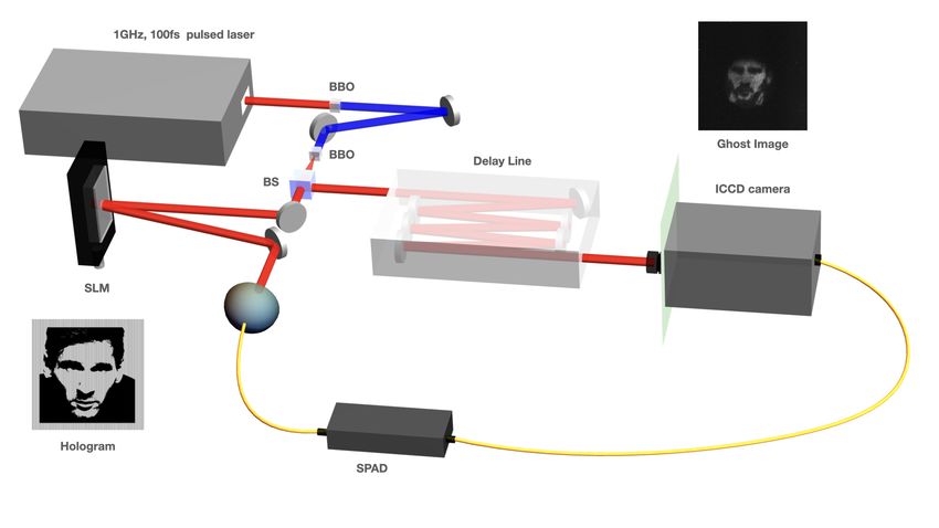
5

called the “Log-determinant divergence” [39, 40] defined as,          circuit for the computation of trace is discussed in the Sup-
                                                                      plementary Information (Figure S2 shows the corresponding
  D(X, Y ) = Tr X · Y −1 − log det X · Y −1 − N, (6)

                                                                      quantum circuit). The whole process which is based on QFT
                                                                      and QFT−1 has a complexity of O(log N ).
where N is the dimension of the matrices. When D = 0, the
matrices X and Y are completely matched, and higher the
distance value the more different are the matrices. The least         TABLE II. Summary of estimated complexities in quantum face
value among the all distance values identifies the best match         recognition algorithm.
and consequently recognizes the face. As it is seen in the                   Method                 Output          Complexity Ref.
distance formula, it is a benefit to be able to calculate the trace           QPCA                 Eigenfaces         log N     [7]
and the determinants of matrices with speedup to expedite the             QICA & HHL            Face components       log N    [23]
distance calculation. In the following, we propose quantum                     HHL              Matrix inversion      log N    [23]
algorithms for computation of the determinant and the trace                Our method        Determinant calculation N log N CW
of a sparse matrix.                                                        Our method           Trace calculation     log N    CW
                                                                        Log-det divergence       Face matching       N log N CW
Quantum Computation of Sparse Matrix Determinants                      Our method (General)     Face recognition     N log N CW
and Trace: To obtain a measure of dissimilarity between two
matrices we need to calculate the determinant and the trace              QPCA and QICA both have logarithmic complexities,
of the sparse matrix A = X · Y −1 . First we calculate Y −1           i.e., O(log N ). For the calculation of the log determi-
using the HHL algorithm [23] and obtain A by multiplying it           nant divergence, the computation of trace has a complex-
with X. We then apply the Quantum Phase Estimation (QPE)              ity of O(log N ), while the determinant has complexity of
subroutine, which consists of a quantum Fourier transform             O(N log N )). Hence, the overall complexity of the whole
(QFT) followed by a controlled Unitary (CU) operation, with           algorithm is O(N log N ). Table II shows a summary of es-
U = e−iA t , and a inverse quantum Fourier transform. We              timated complexities along with the complexity of the general
then apply a controlled Rotation operation followed by the            quantum face recognition algorithm.
inverse Quantum Phase Estimation (QPE) subroutine. At the
end we have a multiplication operator Π which finally gives
us the product of the eigenvalues – the algorithm steps are                                  CONCLUSION
explained in more detail in the Supplementary Information.
The running time of the algorithm up to the third step, i.e. ap-         In summary, we propose a new concept of a quantum pro-
plying the controlled-U operator, is O(log N (s2 κ2 /)) [23],        tocol for 2D face recognition, combining the benefits of quan-
where s is the sparsity, κ is the ratio of largest eigenvalue to      tum imaging in image acquisition with the speedup from the
the smallest eigenvalue of A, and  is the acceptable error.          quantum machine learning algorithms. In this concept, we
Additionally, the multiplication operation in the last step can       consider images to be obtained via a ghost imaging protocol
be performed in time O(log N ) and the algorithm should run           either as inputs to the quantum memories or as a hardware en-
N times. Therefore, the overall
                                  complexity of the algorithm        coding of quantum information for the photonic pattern recog-
is O N log N (1 + s2 κ2 /) , which is much faster than the           nition processor. Feeding the “images” directly from a quan-
classical ones (see Table I).                                         tum protocol also eliminates the need for the conversion of
                                                                      classical data to quantum inputs for the processor saving valu-
                                                                      able computational resources. The quantum pattern recog-
TABLE I. A Comparison of complexities between the classical ap-
                                                                      nition processor then runs an algorithm composed of three
proaches and our quantum approach, current work (CW), for the
computation of determinant.                                           main subroutines: (1) quantum principal components anal-
                                                                      ysis (QPCA), (2) quantum independent component analysis
      Approach          Method        Complexity Ref.
                                                                      (QICA), and (3) quantum dissimilarity measures for compar-
        Classic        Laplace          N3             [41]           ing faces. For the QPCA and QICA, we propose slight mod-
        Classic       Gaussian          N3             [41]
                                                                      ifications in the existing algorithms, whereas for finding the
        Classic Coppersmith-Winogard N 2.373           [42]
                                                                      dissimilarity measure, we propose a novel algorithm for ob-
        Classic     Wiedemann        N 2 log N         [43]
       Quantum      Our method       N log N           CW             taining the distance between two matrices based upon a metric
                                                                      called log-determinant divergence. Our algorithm obtains the
                                                                      determinant and the trace of the two matrices in O(N log N )
                                                                      time – N is the dimension of the matrix. Complexity analysis
  In order to compute the trace of the matrix A, an adder
                                                                      shows that all of the three parts have speedup as compared to
quantum algorithm [44] can speedup the computation. The
                                                                      their classical counterparts, with the overall complexity given
adder operation between two diagonal elements is mainly
                                                                      by O(N log N ). Our conceptual protocol provides a frame-
based on the quantum Fourier transform (QFT), i.e. |Φ(a)i :=
                 PN −1 2πak                                           work for an intelligent and fully quantum image recognition
QFT |ai = √1N k=0 ei N |ki and the inverse QFT, i.e.,                 system with quantum inputs and a quantum machine learning
QFT−1 |Φ(a)i = |ai. By continuation of this method sequen-            processor. The joint benefits of the quantum image acquisition
tially for the all diagonal elements, one can obtain the trace of     and quantum machine learning promises exciting technologi-
the matrix. The detail of the adder algorithm and the quantum         cal developments in the field of image recognition systems.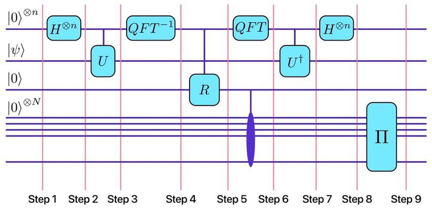
6

 [1] Jeffrey H Shapiro and Robert W Boyd, “The physics of                       Kaler, Isaac L Chuang, and Rainer Blatt, “Implementation of
     ghost imaging,” Quantum Information Processing 11, 949–993                 the deutsch–jozsa algorithm on an ion-trap quantum computer,”
     (2012).                                                                    Nature 421, 48–50 (2003).
 [2] Giorgio Brida, Marco Genovese, and I Ruo Berchera, “Experi-         [21]   Stefanie Barz, Ivan Kassal, Martin Ringbauer, Yannick Ole
     mental realization of sub-shot-noise quantum imaging,” Nature              Lipp, Borivoje Dakić, Alán Aspuru-Guzik, and Philip Walther,
     Photonics 4, 227–230 (2010).                                               “A two-qubit photonic quantum processor and its application
 [3] Mankei Tsang, Ranjith Nair, and Xiao-Ming Lu, “Quan-                       to solving systems of linear equations,” Scientific reports 4, 1–
     tum theory of superresolution for two incoherent optical point             5 (2014).
     sources,” Physical Review X 6, 031033 (2016).                       [22]   Bruce A Draper, Kyungim Baek, Marian Stewart Bartlett, and
 [4] et al. J. Wright, “Robust face recognition via sparse representa-          J Ross Beveridge, “Recognizing faces with pca and ica,” Com-
     tion,” IEEE Trans. Patt. Anal. Mach. Intell. 31, 210 (2009).               puter vision and image understanding 91, 115–137 (2003).
 [5] A. Acan O. Toygar, “Face recognition using pca, lda and ica ap-     [23]   Aram W Harrow, Avinatan Hassidim, and Seth Lloyd, “Quan-
     proaches on colored images,” J. Elect. Elect. Eng. 3, 735 (2003).          tum algorithm for linear systems of equations,” Physical review
 [6] Md Khaled Hasan, Md Ahsan, SH Newaz, Gyu Myoung Lee,                       letters 103, 150502 (2009).
     et al., “Human face detection techniques: A comprehensive           [24]   Alexander I Lvovsky, Barry C Sanders, and Wolfgang Tit-
     review and future research directions,” Electronics 10, 2354               tel, “Optical quantum memory,” Nature photonics 3, 706–714
     (2021).                                                                    (2009).
 [7] Seth Lloyd, Masoud Mohseni, and Patrick Rebentrost, “Quan-          [25]   Michał Parniak, Michał Dkabrowski, Mateusz Mazelanik,
     tum principal component analysis,” Nature Physics 10, 631–                 Adam Leszczyński, Michał Lipka, and Wojciech Wasilewski,
     633 (2014).                                                                “Wavevector multiplexed atomic quantum memory via
 [8] Patrick Rebentrost, Masoud Mohseni, and Seth Lloyd, “Quan-                 spatially-resolved single-photon detection,” Nature communi-
     tum support vector machine for big data classification,” Physi-            cations 8, 1–9 (2017).
     cal review letters 113, 130503 (2014).                              [26]   YF Pu, N Jiang, W Chang, HX Yang, C Li, and LM Duan, “Ex-
 [9] Seth Lloyd, Silvano Garnerone, and Paolo Zanardi, “Quantum                 perimental realization of a multiplexed quantum memory with
     algorithms for topological and geometric analysis of data,” Na-            225 individually accessible memory cells,” Nature communica-
     ture communications 7, 1–7 (2016).                                         tions 8, 1–6 (2017).
[10] Jacob Biamonte, Peter Wittek, Nicola Pancotti, Patrick Reben-       [27]   M Bonarota, JL Le Gouët, and T Chaneliere, “Highly multi-
     trost, Nathan Wiebe, and Seth Lloyd, “Quantum machine learn-               mode storage in a crystal,” New Journal of Physics 13, 013013
     ing,” Nature 549, 195–202 (2017).                                          (2011).
[11] F. Petruccione M. Schuld, Supervised Learning with Quantum          [28]   Jian-Shun Tang, Zong-Quan Zhou, Yi-Tao Wang, Yu-Long Li,
     Computers, 3rd ed., 10, Vol. 4 (Springer International Publish-            Xiao Liu, Yi-Lin Hua, Yang Zou, Shuang Wang, De-Yong He,
     ing, The address, 1993).                                                   Geng Chen, et al., “Storage of multiple single-photon pulses
[12] Devin Powell, “Quantum boost for artificial intelligence,” Na-             emitted from a quantum dot in a solid-state quantum memory,”
     ture News (2013).                                                          Nature communications 6, 1–7 (2015).
[13] G Alvarado Barrios, F Albarrán-Arriagada, FA Cárdenas-            [29]   Manjin Zhong, Morgan P Hedges, Rose L Ahlefeldt, John G
     López, G Romero, and JC Retamal, “Role of quantum correla-                Bartholomew, Sarah E Beavan, Sven M Wittig, Jevon J
     tions in light-matter quantum heat engines,” Physical Review A             Longdell, and Matthew J Sellars, “Optically addressable nu-
     96, 052119 (2017).                                                         clear spins in a solid with a six-hour coherence time,” Nature
[14] Francisco A Cárdenas-López, Lucas Lamata, Juan Carlos Reta-              517, 177–180 (2015).
     mal, and Enrique Solano, “Multiqubit and multilevel quantum         [30]   Yu Ma, You-Zhi Ma, Zong-Quan Zhou, Chuan-Feng Li, and
     reinforcement learning with quantum technologies,” PloS one                Guang-Can Guo, “One-hour coherent optical storage in an
     13, e0200455 (2018).                                                       atomic frequency comb memory,” Nature communications 12,
[15] Dilip Paneru, Eliahu Cohen, Robert Fickler, Robert W Boyd,                 1–6 (2021).
     and Ebrahim Karimi, “Entanglement: quantum or classical?”           [31]   Ya-Fen Hsiao, Pin-Ju Tsai, Hung-Shiue Chen, Sheng-Xiang
     Reports on Progress in Physics 83, 064001 (2020).                          Lin, Chih-Chiao Hung, Chih-Hsi Lee, Yi-Hsin Chen, Yong-Fan
[16] David Collins, Ki Wook Kim, William C Holton, Hanna                        Chen, A Yu Ite, and Ying-Cheng Chen, “Highly efficient co-
     Sierzputowska-Gracz, and EO Stejskal, “Nmr quantum com-                    herent optical memory based on electromagnetically induced
     putation with indirectly coupled gates,” Physical Review A 62,             transparency,” Physical review letters 120, 183602 (2018).
     022304 (2000).                                                      [32]   Chao Liu, Zong-Quan Zhou, Tian-Xiang Zhu, Liang Zheng,
[17] N Schuch and J Siewert, “Implementation of the four-bit                    Ming Jin, Xiao Liu, Pei-Yun Li, Jian-Yin Huang, Yu Ma, Tao
     deutsch–jozsa algorithm with josephson charge qubits,” phys-               Tu, et al., “Reliable coherent optical memory based on a laser-
     ica status solidi (b) 233, 482–489 (2002).                                 written waveguide,” Optica 7, 192–197 (2020).
[18] Zhen Wu, Jun Li, Wenqiang Zheng, Jun Luo, Mang Feng,                [33]   Peter A Morris, Reuben S Aspden, Jessica EC Bell, Robert W
     and Xinhua Peng, “Experimental demonstration of the deutsch-               Boyd, and Miles J Padgett, “Imaging with a small number of
     jozsa algorithm in homonuclear multispin systems,” Physical                photons,” Nature communications 6, 1–6 (2015).
     Review A 84, 042312 (2011).                                         [34]   Agedi N Boto, Pieter Kok, Daniel S Abrams, Samuel L Braun-
[19] Shigeki Takeuchi, “Experimental demonstration of a three-                  stein, Colin P Williams, and Jonathan P Dowling, “Quantum
     qubit quantum computation algorithm using a single photon and              interferometric optical lithography: exploiting entanglement to
     linear optics,” Physical review A 62, 032301 (2000).                       beat the diffraction limit,” Physical Review Letters 85, 2733
[20] Stephan Gulde, Mark Riebe, Gavin PT Lancaster, Christoph                   (2000).
     Becher, Jürgen Eschner, Hartmut Häffner, Ferdinand Schmidt-
7
[35] Yonatan Israel, Shamir Rosen, and Yaron Silberberg, “Super- manuscript, and V.S., S.B., and E.K. revised the final version.
sensitive polarization microscopy using noon states of light,”
Physical review letters 112, 103604 (2014). Competing interests: The authors declare that they have no
[36] Kam Wai Clifford Chan, Malcolm N O’Sullivan, and Robert W competing interests.
Boyd, “Two-color ghost imaging,” Physical Review A 79,
033808 (2009).
Data and materials availability: All data needed to evaluate
[37] Yingwen Zhang, Alicia Sit, Frédéric Bouchard, Hugo
Larocque, Florence Grenapin, Eliahu Cohen, Avshalom C the conclusions in the paper are present in the paper and/or
Elitzur, James L Harden, Robert W Boyd, and Ebrahim Karimi, the Supplementary Materials. Additional data related to this
“Interaction-free ghost-imaging of structured objects,” Optics paper may be requested from the authors.
express 27, 2212–2224 (2019).
[38] Dawid Kopczyk, “Quantum machine learning for data scien-
tists,” arXiv preprint arXiv:1804.10068 (2018).
[39] Andrzej Cichocki, Sergio Cruces, and Shun-ichi Amari, “Log-
determinant divergences revisited: Alpha-beta and gamma log-
det divergences,” Entropy 17, 2988–3034 (2015).
[40] Inderjit S Dhillon and Joel A Tropp, “Matrix nearness problems
with bregman divergences,” SIAM Journal on Matrix Analysis
and Applications 29, 1120–1146 (2008).
[41] James R Bunch and John E Hopcroft, “Triangular factorization
and inversion by fast matrix multiplication,” Mathematics of
Computation 28, 231–236 (1974).
[42] Virginia Vassilevska Williams, “Multiplying matrices in o (n2.
373) time,” preprint (2014).
[43] Douglas Wiedemann, “Solving sparse linear equations over fi-
nite fields,” IEEE transactions on information theory 32, 54–62
(1986).
[44] Lidia Ruiz-Perez and Juan Carlos Garcia-Escartin, “Quantum
arithmetic with the quantum fourier transform,” Quantum In-
formation Processing 16, 152 (2017).
Acknowledgments: V. S. is very thankful for several helpful
discussions with Mikel Sanz and Enrique Solano during his
research stay in QUTIS center in Bilbao (Spain) and QuArtist
center in Shanghai (China), both leading by Enrique Solano
who encouraged the idea to be developed. Also, V. S. is very
grateful for useful discussions with Seth Lloyd and Nathan
Wiebe during the Quantum Machin Learning and Biomimetic
Quantum Technologies conference held in Bilbao.
Funding: D. P., M. R. and E. K. acknowledge the support
of Ontario’s Early Researcher Award (ERA), Canada Re-
search Chairs (CRC), and the European Union’s Horizon
2020 Research and Innovation Programme (Q-SORT), grant
number 766970. V. S. is grateful for the financial support
by the Spanish State Research Agency through BCAM
Severo Ochoa excellence accreditation SEV-2017-0718 and
BERC 2018-2021 program. S.B. acknowledges funding by
the Natural Sciences and Engineering Research Council of
Canada (NSERC) through its Discovery Grant, funding and
advisory support provided by Alberta Innovates through
the Accelerating Innovations into CarE (AICE) – Concepts
Program, and support from Alberta Innovates and NSERC
through Advance Grant.
Author contributions: V.S. and D.P. contributed equally to
this work. V.S. and E.K. developed the idea and consulted it
with D.P., S.B., M.R., and E.S. to design the protocol. V.S.,
M.G., and M.Ab. developed the algorithm, D.P. performed
the experiments under the supervision of E.K. All authors
contributed to discussions. V.S., D.P., and E.K. wrote the8
Supplementary Information for:
Quantum Face Recognition Protocol with Ghost Imaging
S1. QUANTUM IMAGING
We elaborate on the experimental details of the image acquisition for the quantum pattern recognition protocol. Spatially
correlated photon pairs, usually called signal and idler photons, are generated from a Spontaneous Parametric Down Conversion
Process (SPDC) by pumping a nonlinear crystal. Utilizing the position and momentum correlations in these down converted
photon pairs, one can non-locally obtain an image of an object that interacted only with the idler photons. The experimental
setup we use is similar to a conventional ghost-imaging setup, see Fig. S1, with our object being a hologram placed in a Spatial
Light Modulator (SLM), a liquid crystal device. We use a 1 GHZ, 100 fs pulsed laser to pump a nonlinear crystal, β-Barium
Borate (BBO), for generating a second harmonic output. We then use the second harmonic beam to pump a Type-I bismuth
triborate (BiBO) crystal for the down conversion of photon pairs. The generated signal and idler pairs are split into two paths,
i.e. the object arm (idler) and the camera arm (signal), via a 50:50 Beamsplitter (BS). The idler photon interacts with the SLM, on
which we display the holograms created by superimposing the original face image with a diffraction grating. The grating sends
only the desired photons from the incident beam to the the first order, which then are coupled to a Single Mode Fibre (SMF)
and sent into a Single Photon Avalanche Diode (SPAD) detector which can be used to trigger the collection of the photons in
the Intensified CCD (ICCD) camera. The images obtained that are shown in Fig. 2 were taken with 0.5 s exposure accumulated
over 300 frames.
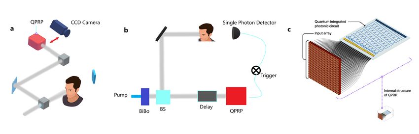
Supplementary Figure S1. Simplified schematic of the experimental setup for Quantum Ghost Imaging. A 1 GHz, 100 fs laser is used to
pump a nonlinear crystal (BBO) for second harmonic generation. The second harmonic beam is used to pump a Type-I bismuth triborate
(BiBO) crystal for entangled photon pair generation. One of the photons is sent to a Spatial Light Modulator, a liquid crystal device, on which
images of human faces are superposed with a diffraction grating. The second photon is sent to a camera through an image preserving delay
line where the image of the object is formed. Figure legends: BiBO - 0.5-mm-thick bismuth triborate crystal; BS - Beamsplitter; BS - Beam
splitter; SPAD - Single Photon Avalanche Diode; ICCD - Intensified CCD camera.9
Supplementary Figure S2. Quantum circuit for the trace calculation of sparse matrix.
S2. QUANTUM COMPUTATION OF TRACE
Here, we suggest an adder algorithm [44] to compute the trace of a matrix via adding the diagonal elements of the matrix
A. This operator is mainly based on quantum Fourier transform (QFT) and inverse QFT (i.e. QFT−1 ). The algorithm should
process the binary forms of the diagonal. For example, the binary representation of the diagonal elements a11 and a22 of
matrix A are respectively a11 = α1 2n−1 + α2 2n−2 + . . . + αn 20 and a22 = β1 2n−1 + β2 2n−2 + . . . + βn 20 , which are
|a11 i = |α1 i ⊗ |α2 i ⊗ . . . |αn i and |a22 i = |β1 i ⊗ |β2 i ⊗ . . . |βn i in the form of quantum kets. The QFT operation on binary
PN −1 i2πak PN −1 −i2πak
state is QFT|ai = √1N k=0 e N |ki and the operation of QFT−1 is QFT−1 |ki = √1N a=0 e N |ai[44]. For simplicity,
we introduce a representation for QFT as
N −1
1 X i2πak
|Φ(a)i = QFT|ai = √ e N |ki,
N k=0
so, we can write
QFT−1 |Φ(a)i = QFT−1 QFT|ai = |ai.
In order to calculate the trace, we need to add all diagonal elements |a11 i + |a22 i + . . . + |aN N i to have the ket include the
value of trace as |a11 + a22 + . . . + aN N i. We introduce the operator Σ that adds two elements a11 and a22 in the form of
|a11 + a22 i as follows:
Σ(|a11 i|Φ(a22 )i) = |Φ(a11 + a22 )i.
Then, after the operation of QFT−1 we obtain
QFT−1 (|Φ(a11 + a22 )i) = |a11 + a22 i.
By continuation of this method for the all diagonal elements, the trace can be obtained. The quantum protocol for computation
of trace is depicted in Fig. S2, in which the input is |a11 i|a22 i . . . |aN N i and the output is |Φ(a11 + a22 + . . . + aN N )i =
|Φ(T r(A))i. Finally, by an operation of QFT−1 we can get |T r(A)i. The whole process based on QFT and QFT−1 has a
complexity log N .10
Supplementary Figure S3. Quantum circuit of determinant calculation of sparse matrix
S3. QUANTUM COMPUTATION OF SPARSE MATRIX DETERMINANTS
Our algorithm for computation of determinant is clarified in the following subsections as inputs, algorithm boxes, and algo-
rithm steps:
1. Inputs
• Sparse matrix A
• |0i⊗n |Ψi as the input in QPE
• |0i as the ancilla for rotation operator
• |0i⊗N as the memory register for multiplication operator
2. Algorithm Boxes
• QPE is the quantum phase estimation subroutine composed of H ⊗n , CU (i.e. controlled-U) and inverse quantum Fourier
transform (QFT−1 )
• Rotation operation (R)
• (QPE)−1 is the inverse operation of QPE, composed of H ⊗n , CU† and quantum Fourier transform (QFT)
• Π is a multiplication operation
2πiA
The matrix A can be exponentiated as the unitary operator U = e 2n with logarithmic complexity [7] in which n is
used in the controlled-U (i.e. CU) part of QPE, and |Ψi is the superposition of the
the precision. This unitary operator is P
eigenvectors of A in the form of |Ψi = βj |uj i. Figure S3 is the representation of the quantum protocol for the computation
of matrix determinants. The following steps are based on the steps shown in Fig. S3.
STEP 1:
The initial state of the algorithm is:
|0i⊗n |Ψi|0i|0i⊗N . (S1)
STEP 2:
After the operation of n Hadamard gates, i.e. H ⊗n , we have:
1
1 X
n |y1 . . . yn i|Ψi|0i|0i⊗N . (S2)
22 y1 ,...,yn =011
STEP 3:
In this step, let us apply the controlled-U (CU) operation:
n
2 −1 N
1 X X 2πiλj y
n βj e 2n |yi|uj i|0i|0i⊗N , (S3)
2 2 y=0 j=1
Pn
where y = l=1 yl 2n−l and λj ’s are the eigenvalues of matrix A.
STEP 4:
Here, we apply the inverse Fourier Transform,
n n
2 −1 2 −1 N λ −k
1 X X X 2πi j2n y
β j e |ki|uj i|0i|0i⊗N . (S4)
2n y=0 j=1
k=0
For a single k among the all possible values, we have λj − k = 0, where λj = x = k. The other terms will be set to zero. Thus,
the notation k is changed to the notation x:
n
2 −1
1 X 2πi λj2n−x y
e =1 (S5)
2n y=0
In this case, the state becomes:
n
2X −1 X
N 1
X N
X
⊗N
βj |λj i|uj i|0i|0i = βj |x1 x2 . . . xn i|uj i|0i|0i⊗N ,
x=0 j=1 x1 ...xn =0 j=1
where
n
X n
X
λj = xl 2n−l = 2n xl 2−l = 2n λ̃j .
l=0 l=0
STEP 5: iσy
In this step, we apply the rotation operation Rl = e 2l , where σy is the Pauli matrix y, which acts on the output of QFT−1 :
1
X N
X q
βj |x1 . . . xn i|uj i( 1 − λ̃2j |0i + λ̃j |1i). (S6)
x1 ...xn =0 j=1
STEP 6:
Applying the quantum Fourier transform (QFT) results in:
n
2 −1 N
1 X X 2πiλj y
q
n βj e 2n |yi|uj i( 1 − λ̃2j |0i + λ̃j |1i). (S7)
2 2 y=0 j=1
STEP 7:
In this step, we apply the CU† operator,
2n −1 N
1 X X
q
n βj |yi|uj i( 1 − λ̃2j |0i + λ̃j |1i). (S8)
2 2 y=0 j=1
STEP 8:
As |uj i’s are known, we repeat the algorithm N times, each time for a specific |uj i, and consequently we obtain the following
state:
Yn q
|0i⊗n |Ψi ( 1 − λ̃2j |0i + λ̃j |1i). (S9)
j=112
Now, the goal is to measure the multiplication of λ̃j ’s in the output of multiplication operation;
N
Y q q q
1 − λ̃2j |0i + λ̃j |1i = 1 − λ̃21 |0i + λ̃1 |1i . . . 1 − λ̃2N |0i + λ̃N |1i (S10)
j
λ̃1 ...λ̃N N
q q q z }| { z }| {
= 1 − λ̃21 ... 1 − λ̃2N |00 . . . 0i + 1 − λ̃21 (λ̃2 ) . . . |0100 . . . 0i + . . . + (λ̃1 )(λ̃2 ) . . . (λ̃N ) |111 . . . 1i . (S11)
. . . 1}i is the term λ̃1 λ̃2 . . . λ̃N in the output of the multiplier, which can be obtained via a weak
The coefficient of the state | |11 {z
N
measurement without collapsing other lines. As λj = 2n λ̃j , we can obtain the determinant of A (i.e. λ1 λ2 . . . λN ) via relation
N
(2n ) λ̃1 λ̃2 . . . λ̃N = λ1 λ2 . . . λN = det(A).
A. Proof of the steps
The proof for each of the eight steps, described above, are given in details in the following expressions.
STEP 2:
n
2 −1
1 X
|Ψ2 i = (H2⊗n ⊗ IN ⊗ I2 ⊗ I⊗N
2 )|0i
⊗n
|Ψi|0i|0i⊗N = n |yi|Ψi|0i|0i⊗N
2 2 y=0
1
1 X
= n |y1 ...yn i|Ψi|0i|0i⊗N (S12)
22 y1 ...yn =0
STEP 3:
n
Y n−l 1
|Ψ3 i = (I⊗l−1
2 ⊗ |0ih0| ⊗ I⊗n−l
2 ⊗ IN ⊗ I2 ⊗ I⊗N
2 + I⊗l−1
2 ⊗ |1ih1| ⊗ I⊗n−l
2 ⊗ U2 ⊗ I2 ⊗ I⊗N
2 ) n ×
l=1
22
1
X N
X
× |y1 ...yn i βj |uj i|0i|0i⊗N
y1 ...yn =0 j=1
1 N n
1 X X Y
= n βj (CU)l |y1 ...yn i|uj i|0i|0i⊗N
22 y1 ...yn =0 j=1 l=1
1 N n
1 X X Y n−l
= n ( βj (δ0,yl + δ1,yl e2πiλ̃j 2 )|y1 ...yn i|uj i|0i)|0i⊗N
22 y
1 ...yn =0 j=1 l=1
1 N n
1 X X Y n−l
= n ( βj e2πiλ̃j yl 2 |y1 ...yn i|uj i|0i)|0i⊗N
22 y
1 ...yn =0 j=1 l=1
1 N
1 X X Pn
yl 2n−l
= n ( βj e2πiλ̃j l=1 |y1 ...yn i|uj i|0i)|0i⊗N
22 y
1 ...yn =0 j=1
n
2X −1 X
N
1
= n βj e2πiλ̃j y |yi|uj i|0i|0i⊗N (S13)
22 y=0 j=113
STEP 4:
n
2 −1 N
−1 1 X X
|Ψ4 i = (QFT ⊗ IN ⊗ I2 ⊗ I⊗N
2 ) n βj e2πiλ̃j y |yi|uj i|0i|0i⊗N
2 2 y=0 j=1
n
2 −1 N
1 X X
= n βj e2πiλ̃j y (QFT−1 |yi)|uj i|0i|0i⊗N
2 2 y=0 j=1
n n
2 −1 N 2 −1
1 X X 1 X −2πi kn y
= n βj e2πiλ̃j y ( n e 2 |kihy|yi)|uj i|0i|0i⊗N
2 2 y=0 j=1 2 2 k=0
n n
2 −1 2 −1 N
1 X X X k
= n βj e2πi(λ̃j − 2n )y |ki|uj i|0i|0i⊗N
2 y=0 j=1 k=0
n n
2X −1 2X −1 X
N
1 λj −k
= βj e2πi( 2n )y |ki|uj i|0i|0i⊗N (S14)
2n y=0 k=0 j=1
n
2X −1 X
N 1
X N
X
|Ψ4 i = βj |λj i|uj i|0i|0i⊗N = βj |x1 x2 ...xn i|uj i|0i|0i⊗N (S15)
x=0 j=1 x1 ...xn =0 j=1
STEP 5:
n
Y
|Ψ5 i = (I⊗n−l+1
2 ⊗ |0ih0| ⊗ I⊗l ⊗N
2 ⊗ IN ⊗ I2 ⊗ I2 + I⊗n−l+1
2 ⊗ |1ih1| ⊗ I⊗l ⊗N
2 ⊗ IN ⊗ Rn−l ) ⊗ I2 ×
l=1
1
X N
X
× |x1 ...xn i βj |uj i|0i
x1 ...xn =0 j=1
1
X N
X n
Y
= βj (CR)n−l+1 |x1 ...xn i|uj i|0i|0i⊗N
x1 ...xn =0 j=1 l=1
1
X N
X n
Y iσy
= βj |x1 ...xn i|uj i( (δ0,xn−l+1 + δ1,xn−l+1 e 2n−l+1 )|0i)|0i⊗N
x1 ...xn =0 j=1 l=1
1 N n
X X Y −(n−l+1)
= βj |x1 ...xn i|uj i( eiσy xn−l+1 2 |0i)|0i⊗N
x1 ...xn =0 j=1 l=1
1 N
xn−l+1 2−(n−l+1)
X X Pn
= βj |x1 ...xn i|uj i(eiσy l=1 |0i)|0i⊗N
x1 ...xn =0 j=1
1
X N
X
= βj |x1 ...xn i|uj i(eiσy λ̃j |0i)|0i⊗N . (S16)
x1 ...xn =0 j=114
STEP 6:
1
X N
X q
|Ψ6 i = (QFT ⊗ IN ⊗ I2 ⊗ I⊗N
2 ) βj |x1 ...xn i|uj i( 1 − λ̃2j |0i + λ̃j |1i)
x1 ...xn =0 j=1
1
X N
X q
= (QFT |x1 ...xn i) βj |uj i( 1 − λ̃2j |0i + λ̃j |1i)
x1 ...xn =0 j=1
n
2X −1 1 N
1
q
2πi 2kn y
X X
=( n e |yihk| |x1 ...xn i) βj |uj i( 1 − λ̃2j |0i + λ̃j |1i)
22 y=0 x1 ...xn =0 j=1
n
−1
2X 1 N
1
q
k
X X
=( n e2πi 2n y |yi hk|x1 ...xn i) βj |uj i( 1 − λ̃2j |0i + λ̃j |1i)
22 y=0 x1 ...xn =0 j=1
n
2X −1 1 N
1
q
k
X X
=( n e2πi 2n y |yi δk,x1 ...xn ) βj |uj i( 1 − λ̃2j |0i + λ̃j |1i)
22 y=0 x1 ...xn =0 j=1
n
2X −1 N
1
q
k
X
=( n e2πi 2n y |yiδk,λj ) βj |uj i( 1 − λ̃2j |0i + λ̃j |1i)
22 y=0 j=1
n
2X −1 N
1 λj X q
= n e2πi 2n y |yi βj |uj i( 1 − λ̃2j |0i + λ̃j |1i)
22 y=0 j=1
n
2X −1 X
N
1 λj
q
= n βj e2πi 2n y |yi|uj i( 1 − λ̃2j |0i + λ̃j |1i) (S17)
22 y=0 j=1
STEP 7:
n
Y n−l
|Ψ7 i = (I⊗l−1
2 ⊗ |0ih0| ⊗ I⊗n−l
2 ⊗ IN ⊗ I2 ⊗ I⊗N
2 + I⊗l−1
2 ⊗ |1ih1| ⊗ I⊗n−l
2 ⊗ (U † )2 ⊗ I2 ⊗ I⊗N
2 )×
l=1
n
2 −1 N
1 X X λj
q
× n βj e2πi 2n y |yi|uj i( 1 − λ̃2j |0i + λ̃j |1i)
2 2 y=0 j=1
1 N n
1 X X λj Y q
= n βj e2πi 2n y (CU† )l |y1 ...yn i|uj i( 1 − λ̃2j |0i + λ̃j |1i)
22 y1 ...yn =0 j=1 l=1
1 N n
1 X X λj Y n−l
q
= n ( βj e2πi 2n y (δ0,yl + δ1,yl e−2πiλj 2 )|y1 ...yn i|uj i( 1 − λ̃2j |0i + λ̃j |1i)
22 y
1 ...yn =0 j=1 l=1
1 N n
1 X X λj Y n−l
q
= n ( βj e2πi 2n y e−2πiλj yl 2 |y1 ...yn i|uj i( 1 − λ̃2j |0i + λ̃j |1i)
22 y
1 ...yn =0 j=1 l=1
1 N
1 λj Pn q
yl 2n−l
X X
= n ( βj e2πi 2n y e−2πiλj l=1 |y1 ...yn i|uj i( 1 − λ̃2j |0i + λ̃j |1i)
22 y
1 ...yn =0 j=1
1 N
1 X X λj
q
= n ( βj e2πi 2n y e−2πiλ̃j y |y1 ...yn i|uj i( 1 − λ̃2j |0i + λ̃j |1i)
22 y
1 ...yn =0 j=1
n
2X −1 X
N
1
q
2πi
= n βj e 2n (λj −λj )y |yi|uj i( 1 − λ̃2j |0i + λ̃j |1i)
22 y=0 j=1
n
2X −1 X
N
1
q
= n βj |yi|uj i( 1 − λ̃2j |0i + λ̃j |1i). (S18)
22 y=0 j=115
STEP 8:
n
2 −1 N
1 X X
q
|Ψ8 i = (H2⊗n ⊗ IN ⊗ I2 ⊗ I⊗N
2 ) n βj |yi|uj i( 1 − λ̃2j |0i + λ̃j |1i)
2 2 y=0 j=1
N
X q
= |0i⊗n βj |uj i( 1 − λ̃2j |0i + λ̃j |1i) (S19)
j=1
N
Y q q q
1 − λ̃2j |0i + λ̃j |1i = 1 − λ̃21 |0i + λ̃1 |1i . . . 1 − λ̃2N |0i + λ̃N |1i
j
λ̃1 ...λ̃N N
q q q z }| { z }| {
= 1 − λ̃21 ... 2
1 − λ̃N |00 . . . 0i + 2
1 − λ̃1 (λ̃2 ) . . . |0100 . . . 0i + . . . + (λ̃1 )(λ̃2 ) . . . (λ̃N ) |111 . . . 1i (S20)You can also read