Bayesian Parameter Tuning of the Ant Colony Optimization Algorithm
←
→
Page content transcription
If your browser does not render page correctly, please read the page content below

DEGREE PROJECT IN TECHNOLOGY,
FIRST CYCLE, 15 CREDITS
STOCKHOLM, SWEDEN 2021

Bayesian Parameter Tuning of the
Ant Colony Optimization Algorithm
Applied to the Asymmetric Traveling Salesman
Problem

KLAS WIJK

EMMY YIN

KTH ROYAL INSTITUTE OF TECHNOLOGY
SCHOOL OF ELECTRICAL ENGINEERING AND COMPUTER SCIENCE
Bayesian Parameter Tuning of
the Ant Colony Optimization
Algorithm
Applied to the Asymmetric Traveling
Salesman Problem

KLAS WIJK
EMMY YIN

Degree Project in Computer Science, DD150X
Date: June 2021
Supervisor: Richard Glassey
Examiner: Pawel Herman
School of Electrical Engineering and Computer Science
Swedish title: Bayesiansk parameterjustering av
myrkolonioptimering: Tillämpat på det asymmetriska
handelsresandeproblemet
iii

Abstract
The parameter settings are vital for meta-heuristics to be able to approximate
the problems they are applied to. Good parameter settings are difficult to find
as there are no general rules for finding them. Hence, they are often manu-
ally selected, which is seldom feasible and can give results far from optimal.
This study investigated the potential of tuning meta-heuristics using a hyper-
parameter tuning algorithm from the field of machine learning, where param-
eter tuning is a common and well-explored area. We used Bayesian Optimiza-
tion, a state-of-the-art black-box optimization method, to tune the Ant Colony
Optimization meta-heuristic. Bayesian Optimization using the three differ-
ent acquisition functions Expected Improvement, Probability of Improvement
and Lower Confidence Bound, as well as the three functions combined using
softmax, were evaluated and compared to using Random Search as an opti-
mization method. The Ant Colony Optimization algorithm with its parame-
ters tuned by the different methods was applied to four Asymmetric Traveling
Salesman problem instances. The results showed that Bayesian Optimization
both leads to better solutions and does so in significantly fewer iterations than
Random Search. This suggests that Bayesian Optimization is preferred to Ran-
dom Search as an optimization method for the Ant Colony Optimization meta-
heuristic, opening for further research in tuning meta-heuristics with Bayesian
Optimization.
iv

Sammanfattning
Bra val av parametrar är avgörande för hur väl meta-heuristiker lyckas approx-
imera problemen de tillämpas på. Detta kan emellertid vara svårt eftersom
det inte finns några generella riktlinjer för hur de ska väljas. Det gör att para-
metrar ofta ställs in manuellt, vilket inte alltid är genomförbart och dessutom
kan leda till resultat långt från det optimala. Att ställa in hyperparametrar är
dock ett välutforskat problem inom maskininlärning. Denna studie undersöker
därför möjligheten att använda algoritmer från maskininlärningsområdet för
att ställa in parametrarna på meta-heurstiker. Vi använde Bayesiansk optime-
ring, en modern optimeringsmetod för optimering av okända underliggande
funktioner, på meta-heuristiken myrkolonioptimering. Bayesiansk optimering
med förvärvsfunktionerna förväntad förbättring, sannolikhet för förbättring
och undre förtroendegräns, samt alla tre kombinerade med softmax, utvärdera-
des och jämfördes med slumpmässig sökning som en optimeringsmetod. Myr-
kolonioptimering vars parametrar ställts in med de olika metoderna tillämpa-
des på fyra instanser av det asymmetriska handlesresandeproblemet. Resulta-
ten visade på att Bayesiansk optimering leder till bättre approximeringar, som
kräver signifikant färre iterationer att hitta jämfört med slumpmässig sökning.
Detta indikerar att Bayesiansk optimering är att föredra framför slumpmässig
sökning, och öppnar för fortsatt forskning av Bayesiansk optimering av meta-
heuristiker.
Nomenclature

Abbreviations

ACO             Ant Colony Optimization algorithm

ACOATSP         Ant Colony Optimization algorithm applied to the Asymmet-
                ric Traveling Salesman Problem

ATSP            Asymmetric Traveling Salesman Problem

BO              Bayesian Optimization

EI              Expected Improvement

LCB             Lower Confidence Bound

PI              Probability of Improvement

RS              Random Search

TSP             Traveling Salesman Problem

Glossary

Black-box Optimization Optimization without knowledge of the underlying
              function

NP-hard Problem A problem that is at least as difficult as the most difficult
             problems in NP, the class of decision problems where yes-
             instances are verifiable in polynomial time

                                     v
Contents
1 Introduction 1
1.1 Research Question . . . . . . . . . . . . . . . . . . . . . . . 2
1.2 Scope . . . . . . . . . . . . . . . . . . . . . . . . . . . . . . 2
2 Background 3
2.1 Traveling Salesman Problem . . . . . . . . . . . . . . . . . . 4
2.2 Meta-heuristics . . . . . . . . . . . . . . . . . . . . . . . . . 4
2.2.1 Ant Colony Optimization . . . . . . . . . . . . . . . . 4
2.3 Parameter Tuning . . . . . . . . . . . . . . . . . . . . . . . . 7
2.3.1 State of the Art . . . . . . . . . . . . . . . . . . . . . 7
2.3.2 Random Search . . . . . . . . . . . . . . . . . . . . . 7
2.3.3 Bayesian Optimization . . . . . . . . . . . . . . . . . 8
2.4 Related Work . . . . . . . . . . . . . . . . . . . . . . . . . . 12
3 Methods 14
3.1 Test Methodology . . . . . . . . . . . . . . . . . . . . . . . . 14
3.1.1 Tuning Procedure . . . . . . . . . . . . . . . . . . . . 14
3.1.2 Random Seeding . . . . . . . . . . . . . . . . . . . . 14
3.1.3 Parameter Configuration . . . . . . . . . . . . . . . . 15
3.2 Problem instances . . . . . . . . . . . . . . . . . . . . . . . . 17
3.3 Tools . . . . . . . . . . . . . . . . . . . . . . . . . . . . . . . 17
3.4 Evaluation . . . . . . . . . . . . . . . . . . . . . . . . . . . . 17
4 Results 19
4.1 General Results . . . . . . . . . . . . . . . . . . . . . . . . . 19
4.2 Acquisition Functions . . . . . . . . . . . . . . . . . . . . . . 23
4.2.1 Probability of Improvement . . . . . . . . . . . . . . 23
4.2.2 Expected Improvement . . . . . . . . . . . . . . . . . 25
4.2.3 Lower Confidence Bound . . . . . . . . . . . . . . . 26
4.2.4 Softmax . . . . . . . . . . . . . . . . . . . . . . . . . 27
viCONTENTS vii
5 Discussion 28
5.1 Results . . . . . . . . . . . . . . . . . . . . . . . . . . . . . . 28
5.2 Implications . . . . . . . . . . . . . . . . . . . . . . . . . . . 30
5.3 Limitations and Validity . . . . . . . . . . . . . . . . . . . . 30
5.4 Future Work . . . . . . . . . . . . . . . . . . . . . . . . . . . 31
6 Conclusions 32
Bibliography 33
A Implementation 36
B Statistical tests 37Chapter 1
Introduction
In many areas of computer science, numerical methods and machine learn-
ing, algorithms use external settings or parameters in order to change their
behaviour and performance [1]. Parameters are a general concept which can
have integer, real-number or categorical values. The problem of selecting the
best parameters can be seen as an optimization problem in the space composed
of the parameter values.
A domain in which algorithms with parameters are common is meta-heuristics.
Meta-heuristics are algorithmic templates which are commonly applied to NP-
hard problems. One of the most well-known NP-hard problems is the Traveling
Salesman Problem (TSP). A variant of TSP is the asymmetric TSP (ATSP).
ATSP is not as well studied as the regular, symmetric version of TSP, even
though ATSP also has several real-world applications and is of importance as
well [2]. Regardless, some meta-heuristics, such as the Ant Colony Optimiza-
tion algorithm (ACO) [3], has been shown to have potential for approximating
both TSP and ATSP.
Since meta-heuristic algorithms for NP-hard problems seldom produce
good solutions for all problems or instances of a certain problem, they of-
ten rely on parameters to change their behaviour in accordance to the given
problem or problem instance. There is, however, no general rule for finding
the optimal parameters [4]. In many cases, the parameters of meta-heuristics
such as ACO are tuned by hand, by following conventions or through limited
experimental comparisons [5]. Manually selecting parameters is not always
feasible or time-efficient and does not guarantee any local or global optimum
[6]. Automating this selection could therefore be highly useful. As parame-
ter optimization is a greatly researched area of machine learning, there could
be potential for applying those optimization methods to the problem of tuning
12 CHAPTER 1. INTRODUCTION
parameters in meta-heuristics.
Limited research regarding the effect of optimization algorithms as param-
eter tuning methods on meta-heuristics has been conducted before [4]. How-
ever, Bayesian Optimization (BO), which is one of the most common black-box
optimization methods [7], has not yet been evaluated for tuning parameters of
meta-heuristics. Therefore, this study aims to evaluate BO, with different ac-
quisition functions, as a parameter tuning method for the ACO meta-heuristic
applied to the ATSP (ACOATSP) by comparing it to a random parameter se-
lection method.
1.1 Research Question
How does Bayesian Optimization compare to naive Random Search in opti-
mizing the parameters of the Ant Colony Optimization algorithm when ap-
plied to the Asymmetric Traveling Salesman Problem?
1.2 Scope
BO as a parameter tuning method for ACO, as it was originally proposed [3],
will be evaluated in this study. The focus of the study is to investigate if and
to what extent BO could be considered for automatically tuning the parame-
ters of meta-heuristics. Thus, we will not attempt to map out the specifics of
ACO, such as how its parameters are related to each other, but only look at the
performance of the algorithm after being tuned using BO.
ACO, in turn, will only be applied to ATSP. Evaluating other types of TSP
instances, other NP-hard problems or applying BO to other meta-heuristics
could be of interest, but is not within the scope of this study.Chapter 2
Background
In this study, the components of the tuning problem, as shown in figure 2.1,
are the following: The NP-hard problem is the Asymmetric Traveling Sales-
man Problem, the meta-heuristic is Ant Colony Optimization and, as described
in section 1.1, this study aims to compare the parameter tuning algorithms
Bayesian Optimization and Random Search. Each of these components along
with additional relevant background information will be described in this sec-
tion.
Parameter Tuning Algorithm
Tune parameters
Meta-heuristic
Solve heuristically
NP-Hard Problem
Figure 2.1: Overview of the tuning problem
34 CHAPTER 2. BACKGROUND
2.1 Traveling Salesman Problem
The Traveling Salesman Problem (TSP) is an important problem within com-
binatorical optimization. The problem is to, given a weighted graph, find the
Hamilton cycle with minimal weight, i.e. the shortest tour that visits each node
exactly once and ends in the starting node. The problem has many applications
within computer science and logistics. An example is machine sequencing and
scheduling, where the problem is to find the cheapest order to process a given
set of jobs, with different set up costs between the jobs. [8]
There are many variations of TSP. In the general TSP, the distance from
a to b is equal to the distance from b to a for all nodes a, b. The asymmetric
TSP (ATSP) is a less studied type of TSP. Here, the distance from one node
to another does not have to equal their reversed distance. ATSP is more diffi-
cult than the general TSP to both approximate and optimize. The structure of
ATSP instances together with the great structural variations between each in-
stance can affect the performance of meta-heuristics in both time and memory
requirement [2].
2.2 Meta-heuristics
Meta-heuristics can be seen as general algorithmic templates, and are often
used to approximate solutions. Many problems are too computationally heavy
to solve exactly. Thus, it is common to compute solutions that are not exact
but close to the optimal solution when there are limitations in time or compu-
tational resources. An advantage of using meta-heuristics is that they are not
problem-specific, as opposed to regular heuristics. By adapting the parameters
of meta-heuristics, they can be applied to a wide range of problems [9].
2.2.1 Ant Colony Optimization
The Ant Colony Optimization algorithm was first introduced in the 1990s by
Dorigo [3], and the following section is derived from his work. ACO is a
meta-heuristic comparable to Simulated Annealing and Tabu Search. It was
originally applied to multiple combinatiorical optimization problems, includ-
ing TSP and ATSP, with promising results. The algorithm is inspired by the
way ants communicate information between themselves, in order to find the
shortest paths between feeding sources and the colony. Ants leave pheromone
trails which other ants pick up on and follow, further increasing the pheromone
level of a trail. If put in a new environment, the shortest path to a food sourceCHAPTER 2. BACKGROUND 5
will eventually have the strongest trail, resulting in all the ants choosing that
shortest path. In ACO, parameters for the relative importance of the trail, the
relative importance of the visibility, trail persistence, the number of ants and
a constant related to the quantity of trail laid by ants are used to simulate this
behaviour. The parameters are presented in table 2.1.
Table 2.1: The parameters used in ACO.
Parameter Interpretation
α The relative importance of the trail
β The relative importance of the visibility
ρ Trail persistence
Q A constant related to the quantity of trail laid by ants
m The number of ants
Artificial ants make up the ACO algorithm. When used to approximate
TSP, an artificial ant will move from node to node until all n nodes have been
visited exactly once, and then return to the starting node. In each iteration,
every ant chooses to move from its current position to a new, unvisited node.
After n iterations, all ants have completed a tour. The pheromone levels of the
edges are then updated. If τij (t) is the trail intensity of edge (i, j) at time t,
the updated intensity of that edge will be as shown in equation 2.1.
m
X
τij (t + n) = ρ ∗ τij (t) + ∆τijk (t) (2.1)
k=1
LQ , if kth ant used edge (i, j)
k k in its just completed tour
∆τij (t) = (2.2)
0,
otherwise
τij (t + n) is calculated using each ant’s tour and the tour’s total length L, to-
gether with the parameters ρ and Q. τij affect the probability that edge (i, j)
is chosen by an ant in the following iterations. The choices are however regu-
lated by keeping tabu lists for the ants, in order to force legal tours. Equation
2.3 gives the probability of ant k moving from node i to node j at time t.
α β
P [τij (t)] ∗[ηijα] β, if j ∈ allowedk
pkij (t) = k∈allowedk [τik (t)] ∗[ηik ] . (2.3)
0, otherwise6 CHAPTER 2. BACKGROUND
α is the relative importance of the trail and β the relative importance of the vis-
ibility. Equation 2.3 can thus be interpreted as a trade-off between the weight
of edge (i, j), and the number of preceding ants choosing that edge. Simi-
lar to real ant colonies, the artificial ants will eventually choose shorter paths,
resulting in better approximations of TSP.
The pseudo-code for ACO is presented below in algorithm 1.
Algorithm 1: Ant Colony Optimization
Input: α, β, ρ, Q, m (see table 2.1), number of cycles N Cmax
Output: The shortest tour estimated by the algorithm
1 t = 0 // time counter
2 NC = 0 // cycles counter
3 for each edge (i, j) do
4 τij = c // some constant c
5 ∆τij = 0
6 while N C < N Cmax do
7 place the m ants on the n nodes
8 s=0 // tabu list index
9 for k = 1, 2, . . . , m do
10 place the starting node of ant k in tabuk (s)
11 while tabu list is not full do
12 s=s+1
13 for k = 1, 2, . . . , m do
14 choose node j with probability pkij (t) // eq. 2.3
15 move ant k to node j
16 tabuk (s) = tabuk (s) ∪ j
17 for k = 1, 2, . . . , m do
18 move ant k to its starting node
19 compute Lk
20 update shortest tour found
21 for each edge (i, j) do
22 for k = 1, 2, . . . , m do
23 update ∆τijk // eq. 2.2
k
24 ∆τij = ∆τij + ∆τij
25 for each edge (i, j) do
26 compute τij (t + n) // eq. 2.1
27 t=t+n
28 NC = NC + 1
29 return shortest tourCHAPTER 2. BACKGROUND 7
2.3 Parameter Tuning
Meta-heuristic algorithms are heavily reliant on their parameters in order to
solve optimization problems. Without the correct parameter settings, meta-
heuristic algorithms may exhibit undesired behaviour, such as converging at
local optima and stagnating, resulting in poor solutions [10]. The optimal pa-
rameters for a meta-heuristic algorithm vary both depending on which prob-
lem and which problem instances the algorithm is applied to. In this study, the
parameter tuning problem will be considered as the optimization problem of
minimizing the cost of the underlying problem’s solution as a function of the
meta-heuristic’s parameters, within a feasible set of parameters (search space).
Thus, in this context, the objective function is ACO and its possible parameter
settings form a search space which the chosen optimization methods (RS and
BO) aim to find the specific setting (point) that yields the shortest tour for a
given ATSP instance.
2.3.1 State of the Art
Historically, parameter tuning within academic settings has often been done
manually, through experiments, or adopting values that had previously worked
in a similar settings [9]. This is the case in the widely used Python library
SciPy, where the selection of parameters for the Basin-hopping meta-heuristic
algorithm are left to the user [11]. However, in the last two decades, a number
of automatic parameter tuning approaches have been suggested [9], notably
the F-Race algorithm [4].
2.3.2 Random Search
The Random Search algorithm is a naive approach to global optimization. The
algorithm selects random points in the search space and compares them to the
best value found.
The pseudo-code for RS is presented below in algorithm 2.8 CHAPTER 2. BACKGROUND
Algorithm 2: Random Search (Minimization)
Input: Objective function f , Number of iterations k
Output: Estimate x̂ of arg minx f (x)
1 ymin = ∞
2 x̂ = null
3 for n = 1, 2, . . . , k do
4 select a random point x ∈ A
5 yx = f (x)
6 if yx < ymin then
7 ymin = yx
8 x̂ = x
9 return x̂
An alternative to the Random Search algorithm is the Grid Search al-
gorithm. Instead of selecting points at random, Grid Search selects evenly
spaced points in the search space. Although Grid Search is predictable and
interpretable, it often produces inferior results compared to Random Search
in practice [7].
2.3.3 Bayesian Optimization
Bayesian Optimization is an iterative algorithm for black-box optimization. It
is a state-of-the-art technique for computationally expensive functions, and has
been successfully applied to the tuning of Deep Neural Networks in a number
of applications [7].
There are two main components of BO. A surrogate function f ∗ and an
acquisition function u. The surrogate function provides a probabilistic model
of the true objective function. The acquisition function is a function which,
according to some rule, transforms the surrogate function to real values that
express how important each point is to evaluate. The maximum of the acqui-
sition is the point that is most important and should be sampled from the true
objective function next.
The main steps of a BO iteration are the following: First, the algorithm
finds the point x ∈ A that maximizes the acquisition function u. Next, the
objective function is evaluated at x. The result, f (x), is then used to update
the surrogate model f ∗ .
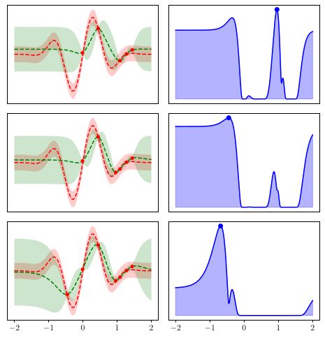
The pseudo-code for BO is presented below in algorithm 3, and example
iterations of BO applied to a minimization problem are shown in figure 2.2.CHAPTER 2. BACKGROUND 9
Algorithm 3: Bayesian Optimization (Minimization)
Input: Objective function f , Number of iterations k, Acquisition
function u
Output: Estimate x̂ of arg minx f (x)
1 ymin = ∞
2 x̂ = null
3 for n = 1, 2, . . . , k do
4 select the point x ∈ A that maximizes u(x)
5 yx = f (x)
6 if yx < ymin then
7 ymin = yx
8 x̂ = x
9 update f ∗ using yx
10 return x̂
Figure 2.2: Illustration of BO. Each row shows one consecutive iteration of
BO. Left column: The red dotted line is the true function and the green dotted
line the surrogate model, and the corresponding shadowed areas are the surro-
gate model’s confidence interval. The red points are the previously evaluated
points. Right column: The acquisition function. The point where the graph is
at its maximum will be the point evaluated next.10 CHAPTER 2. BACKGROUND
Surrogate model
A popular choice of surrogate model, and the type of surrogate model used
in this study, is a Gaussian process. Gaussian processes use different kernel
functions to encode assumptions about the objective function, and thus model
it more accurately given that the assumptions are reasonably correct. Common
kernel functions include the exponential kernel, the polynomial kernel and the
Matérn kernel. These kernel functions share the assumption that points that
are close to each other are likely to be similar. The Matérn kernel provides
a parameter ν that controls smoothness. This kernel is k times differentiable
where ν > k, k ∈ N. In machine learning settings, the parameter values
ν = 5/2 and ν = 3/2 are suitable [12].
The kernel function allows BO to model noisy objective functions. A basic
approach for modelling the noise is to additively combine a main kernel which
represents the noiseless part of the objective function with some other kernel
that represents the noise. This approach assumes that equation 2.4 holds for
the objective function.
f (x) = g(x) + (2.4)
where f (x) is the objective function, g(x) is the noiseless objective function
and is an error function. In terms of the kernel function, g(x) and corre-
spond to the main kernel and the noise kernel respectively. A simple choice
of noise kernel is a White kernel which models the noise as distributed identi-
cally and independently Gaussian. In the BO setting, the variance of the noise
can either be estimated based on the data or set ahead of time.
Acquisition Function
The choice of acquisition function determines the algorithm’s behaviour. Three
common choices of acquisition functions are Probability of Improvement, Ex-
pected Improvement and Lower Confidence Bound [13]. Ideally, the acqui-
sition function does a good job balancing the trade-off between exploratory
and exploitative evaluations. For the acquisition functions below, real valued
parameters (ξ and κ) can be used to control this trade-off.
Probability of Improvement (PI) (equation 2.5) is an acquisition function
which expresses the probability that a candidate evaluation point x results in
a greater objective function value than the best known point. The parameter ξ
is used to control how much the value should improve.
P I(x) = P r(f ∗ (x) < f ∗ (xbest ) + ξ) (2.5)CHAPTER 2. BACKGROUND 11
Expected Improvement (EI) (equation 2.6) expresses the expected value of
the difference of the objective function’s value in a candidate point x and the
best known point. EI(x) can be written as a closed form expression, intro-
ducing the parameter ξ which controls the amount of improvement from the
previous best values [13].
EI(x) = E[f ∗ (xbest ) − f ∗ (x)] (2.6)
Lower Confidence Bound (LCB) (equation 2.7) simply returns an upper
confidence bound from the (Gaussian process) surrogate function. The pa-
rameter κ is used to control which confidence bound should be considered.
LCB(x) = µGP − κσGP (2.7)
Combining the above acquisition functions, PI, EI and LCB, using the soft-
max function (equation 2.8) results in a new acquisition function. This poten-
tially results in a more balanced acquisition function since it weighs several
factors in the decision.
( )
eP I(x) , eEI(x) , eLCB(x)
Sof tmax(x) = max (2.8)
eP I(x) + eEI(x) + eLCB(x)
Initial Sampling
There are some time or iteration dependent methods that can be employed to
avoid exploiting a local optimum too early. One such method is to dedicate
the first n function evaluations to initial sampling. This is done in order to get
enough samples to model the search space using the surrogate function in a
meaningful way before starting the BO, and simultaneously observe enough
points to have some alternative areas to explore when areas have been suffi-
ciently exploited. How the initial sampling should be done is a research area
of its own, but some alternatives are random, latin hypercube, Hammersely
and Halton sampling. While completely random sampling can be a viable op-
tion, it is in many cases preferable to perform the initial sampling such that the
samples are more evenly spaced out, using a low discrepancy sampling method
[14]. The differing effects of using random sampling and a low discrepancy
sampling method is illustrated in figure 2.3.12 CHAPTER 2. BACKGROUND
Figure 2.3: An illustration of random sampling compared to a low discrepancy
sampling method. Left: Random sampling. Right: Low discrepancy sampling
using a Hammersley sequence [15].
2.4 Related Work
Due to the importance of the parameter settings for meta-heuristics, a large
number of automatic tuning methods with various approaches have previously
been proposed.
Smit and Eiben [5] compared three different parameter tuning methods for
evolutionary algorithms, a field of population-based meta-heuristic algorithms
that ACO can be considered a sub-field of. Two of the tuning methods, CMA-
ES and REVAC, used an evolutionary approach to optimize the parameters
and can be seen as heuristic search-based tuning methods [9]. The third tun-
ing method was a sequential parameter optimization method, SPO, which is
a model-based approach [9]. The results indicated that using either algorithm
to tune the parameters are much more efficient than tuning the parameters by
hand, following conventions or pure intuition.
Hutter, Hoos and Stützle [16] proposed the method ParamILS which is
based on iterative local search. ParamILS is applicable to various algorithms,
regardless of the number of parameters, tuning scenario and objective.
Li and Zhu [6] used an evolutionary algorithm called Bacterial Foraging
Algorithm to optimize the parameters of ACO, comparing it to a genetic al-
gorithm and a particle swarm optimization algorithm, which all are heuristic
search-based methods. They concluded that the Bacterial Foraging Algorithm
was a good method for selecting parameters of ACO.CHAPTER 2. BACKGROUND 13
Birattari and Kacprzyk [4] discussed the potential of using machine learn-
ing methods to tune meta-heuristics. They compare the parameter tuning
problem to optimization problems within machine learning, inferring that the
similarities should make machine learning approaches considered for param-
eter tuning. These can be categorized as numerical optimization-based tuning
methods [9]. Some empirical analyses were made, including experimental ap-
plication of racing algorithms on ACO for solving TSP. The results showed
that the F-Race approach was up to 10 times more efficient than a brute-force
approach. An extension of this idea is to combine it with statistical techniques
[17]. Barbosa and Senne [17] used Design of Experiments together with rac-
ing algorithms to construct a method called HORA. A case study was per-
formed using HORA on the meta-heuristics simulated annealing and genetic
algorithm to solve TSP. Their results showed that this method was more effec-
tive and gave better results compared to only using a racing algorithm.
There are several other proposed methods which has been applied to other
meta-heuristics. A similarity among the methods are that they are black-box
optimization methods, of which BO is a state-of-the-art technique commonly
used in machine learning [7]. Though some machine learning methods has
been explored [4], little has been investigated regarding BO as a parameter
tuning method for ACOATSP. Through this study, additional insight to using
such methods for tuning meta-heuristics can be contributed.Chapter 3
Methods
3.1 Test Methodology
3.1.1 Tuning Procedure
Each optimization method (RS or BO) was evaluated by tuning the parame-
ters of ACO to solve a given ATSP instance. The optimization methods were
implemented according to section 2.3.2 and 2.3.3. For the tuning procedure,
300 iterations of an optimization method were used. In each iteration, 200
calls within the objective function was made, i.e. we set N Cmax = 200 in
algorithm 1. A record was kept of the shortest tour length found. After com-
pleting one iteration, the currently shortest tour was compared to the resulting
tour length and updated thereafter. Then a new iteration of the optimization
method was initiated until completing a total of 300 iterations. Due to the tun-
ing procedure’s stochastic nature, it was repeated 24 times for each instance to
gather statistical data.
3.1.2 Random Seeding
There is a certain randomness to ACO, as well as RS. The pseudo-random
number generation used in the implementation was seeded such that the re-
sults are replicable and comparable. Each of the 24 repeated runs of the tuning
procedures had a unique random seed as to create 24 different runs. The ob-
jective function (ACO) was seeded such that the sequence of values obtained
when repeatedly sampling the same point depends on the random seed and is
independent of what other points have been previously sampled. This makes
sure that sampling the same points for a given run, including repeated sam-
14CHAPTER 3. METHODS 15
pling, results in the same set of function values, i.e. tour lengths, regardless of
sampling order. Repeating one specific run therefore generates the exact same
result. To determine which points should be considered the same, a minimum
distance was used. If two points are less than the minimum distance apart, they
were considered to be the same, thus advancing that point’s random seeding
sequence one step. The minimum distance threshold was chosen to be small,
10−8 . A small value was chosen in order to avoid advancing the random seed-
ing sequence when two points that already yield slightly different function
values (tours) are sampled.
3.1.3 Parameter Configuration
Search Space
The parameters of the ACO span an infinite search space A, since at least one
of the parameters span an infinite range. Solving the tuning problem with an
infinite search space is not feasible. In order to provide a finite search space,
we defined finite ranges for all parameters. Furthermore, it has been observed
that some parameter values are unlikely to result in good configurations [3].
The ranges which each of the parameters were evaluated within are shown in
table 3.1, and were based on previous work by Dorigo [3].
Table 3.1: Parameter ranges for the ACOATSP. All ranges are in R.
Parameter Feasible set Chosen search space
α [0, ∞) [0, 5]
β [0, ∞) [0, 5]
ρ [0, 1) [0.1, 0.99]
Q [0, ∞) [1, 100]
The number of ants m was chosen to be equal to the number of vertices in
the ATSP instance and the cycles within ACO N Cmax = 200.
Bayesian Optimisation
The following BO model was used in the study. An initial sampling of 25
evaluations was performed using Hammersely sampling. Low discrepancy
sampling was chosen because it was deemed likely to be more effective than16 CHAPTER 3. METHODS
random sampling (see section 2.3.3), but the specific choice of low discrep-
ancy sampling was not within the scope of this study and thus arbitrary. The
kernel used was a Matèrn kernel with ν = 5/2, additively combined with
a White kernel to model the noise. The kernel is the default kernel in the
Scikit-Optimize library and has been successfully applied in parameter tuning
of machine learning models [18]. The variance of the White kernel was set
to a constant, instead of estimating the variance during the optimization. This
was done because, contrary to the modelling assumption, the noise of the ob-
jective function is not independently identically distributed Gaussian. This is
most clear when sampling poor areas of the search space, which results in a
substantially greater noise. These poor areas are not of interest when running
the BO, but made the variance estimate unreliable. Hence, the variance was
set to 0.7. Setting the variance to a constant partially solved these problems,
but made the optimization underestimate poor areas of the search space. This
inaccuracy in the modelling was considered an improvement overall, since it
did not matter that these already poor areas were underestimated.
Acquisition functions
All three common acquisition functions PI, EI and LCB, and softmax were
tested in order to more accurately evaluate the performance of BO. As the
acquisition functions themselves have parameters to control the exploration
exploitation trade-off, we tested three different settings for each of the acqui-
sition functions. The default setting was used, and an increase and decrease
by a factor of 2. These are presented in table 3.2. For softmax, the underlying
acquisition functions were PI with ξ = 0.01, EI with ξ = 0.01 and LCB with
κ = 1.96.
Table 3.2: The acquisition functions and corresponding parameter values eval-
uated.
Acquisition function Tested settings
PI ξ = 0.005, 0.01, 0.02
EI ξ = 0.005, 0.01, 0.02
LCB κ = 0.98, 1.96, 3.92CHAPTER 3. METHODS 17
3.2 Problem instances
The TSPLIB library [19] was used to find problem instances to evaluate on.
As mentioned in section 1.2, this study is limited to ATSP instances. Further-
more, the instances were chosen based on their size. Due to time constraints
and limited access to computational power, instances with high vertex counts
were omitted. Several instances provided by the TSPLIB library have the same
prefix, indicating that the problems are related. Hence, ATSP instances with
differing prefixes were chosen. The final ATSP instances used were ftv35,
p43, ry48p and ft53. These are all complete graphs. The number of nodes,
optimal tour lengths, and average and median distance between the nodes for
these are presented in table 3.3.
Table 3.3: The ATSP instances used in this study with their number of nodes,
optimal tour length and average and median distance between two different
nodes.
Instance Nodes Optimum Average distance Median distance
ftv35 36 1473 135 133
p43 43 5620 594 25
ry48p 48 14422 1139 1029.5
ft53 53 6905 493 372
3.3 Tools
External tools were used for parts of our implementation. For the optimization
methods (BO and RS), the Scikit-Optimize library implementation was used.
Scikit-Optimize is a Python open-source library for optimization [18]. For
ACO, the libaco library implementation [20] was used. As there were some
limitations to this library, it was modified slightly in order to allow the setting
of the parameter Q (table 2.1), random seeding, and parsing of ATSP instances
from TSPLIB [19].
3.4 Evaluation
The resulting shortest tour lengths produced by the optimization methods were
compared to the optimal tour length for each ATSP instance. In addition, the18 CHAPTER 3. METHODS
tuning procedure was ran using constant parameters, which seems to be com-
mon when applying meta-heuristics [5]. The performance of the optimization
methods could thus be compared to using constant parameters. Due to diffi-
culties in finding conventional parameter settings for ACOATSP, the default
values of the libaco library were used. These were: α = 1.0, β = 1.0, ρ =
0.1, q = 1.
To determine if RS and BO differ significantly, statistical tests were used.
In this study, we considered both Student’s t-test and Wilcoxon signed rank
test, which was used by Brittari and Kacprzyk to evaluate F-Race [4]. The
null hypothesis that was evaluated was: using BO (with a specific acquisition
function) and RS as parameter tuning algorithms for ACOATSP result in equal
tour lengths. A confidence level of 95% is considered significant in this study.
The same statistical tests were employed to determine if there was a difference
between the different acquisition functions.Chapter 4
Results
4.1 General Results
Considering the results for all four ATSP instances, it is clear that the perfor-
mance of ACO varies significantly depending on the instance, and whether BO
or RS is used. While difference between the results obtained using BO and RS
vary for each instance, BO is consistently favoured. Figure 4.1 shows box plots
for each ATSP instance over the 24 runs with RS and BO using softmax, PI,
EI and LCB with default parameters. Each box shows the median, the upper
and lower quartile. The left and right whiskers show values that lie within
1.5 times the interquartile range of the upper and lower quartiles respectively.
Values outside of this whisker range are explicitly shown as circles. The differ-
ence in performance is distinct when applied to ftv35 and p43. When applied
to ry48p and ft53, BO still yields shorter tours than RS, even though the re-
sults fluctuate more. Note that although the box plots provide an overview of
the compiled results, the gathered data is not continuous. Results for ft35 and
p43 belong to a small set of values such that there are seemingly few possible
values and many repeated data points.
1920 CHAPTER 4. RESULTS
ftv35
Random
Softmax
LCB κ = 1.96
EI ξ = 0.01
PI ξ = 0.01
1500 1495 1490 1485 1480 1475
p43
Random
Softmax
LCB κ = 1.96
EI ξ = 0.01
PI ξ = 0.01
5632 5630 5628 5626 5624 5622
ry48p
Random
Softmax
LCB κ = 1.96
EI ξ = 0.01
PI ξ = 0.01
15100 15000 14900 14800 14700 14600 14500 14400
ft53
Random
Softmax
LCB κ = 1.96
EI ξ = 0.01
PI ξ = 0.01
7600 7500 7400 7300 7200
Figure 4.1: Results for the four tested ATSP instances shown as box plots. Top
to bottom: ftv25, p43, ry48p and ft53.CHAPTER 4. RESULTS 21
Table 4.1: The median tour length for each optimization method applied on
each ATSP instance, compared to the optimal tour length.
Instance
ftv35 p43 ry48p ft53
Optimal 1473 5620 14422 6905
Constant 1479 5625 15055.5 7435.5
Random 1499 5629 14917.5 7461
PI (ξ = 0.01) 1473 5626 14765 7391.5
EI (ξ = 0.01) 1475 5627 14703 7391
LCB (κ = 1.96) 1473 5626 14809.5 7344
Softmax 1473 5626 14772 7357
The resulting median tour lengths when ACO was tuned by RS and BO
using default values for the acquisition functions are shown in table 4.1. As the
ATSP instances are of different complexities and have optimal tours of varying
lengths, the results are also shown in table 4.2 as the percentage of the optimal
tour length for each instance, i.e. a measurement of the difference proportional
to the optimal tour length, to enable easier comparisons between the instances.
BO resulted in shorter tours than RS for all of the ATSP instances. When
applied to the smallest instance, ftv35, BO using either PI, LCB or softmax
resulted in the optimal tour length. None of the optimization methods managed
to produce an optimal tour length for the other instances. However, when
looking at the minimum tour lengths produced by the optimization methods,
as presented in table 4.3, BO using LCB yielded the optimal tour length for
ry48p as well as ftv35.22 CHAPTER 4. RESULTS
Table 4.2: The difference in median tour length for each optimization method
applied on each ATSP instance compared to the optimal tour length as a per-
centage of the optimal tour length.
Instance
ftv35 p43 ry48p ft53
Optimal 0 0 0 0
Constant 0.41 0.09 4.39 7.68
Random 1.77 0.16 3.44 8.05
PI (ξ = 0.01) 0 0.11 2.39 7.05
EI (ξ = 0.01) 0.14 0.12 1.95 7.04
LCB (κ = 1.96) 0 0.11 2.69 6.36
Softmax 0 0.11 2.43 6.55
Table 4.3: The minimum tour length for each optimization method applied on
each ATSP instance, compared with the optimal tour length.
Instance
ftv35 p43 ry48p ft53
Optimal 1473 5620 14422 6905
Constant 1473 5622 14763 7232
Random 1477 5625 14459 7336
PI (ξ = 0.01) 1473 5622 14495 7211
EI (ξ = 0.01) 1473 5625 14575 7209
LCB (κ = 1.96) 1473 5623 14422 7176
Softmax 1473 5621 14466 7211
Constant parameters were best for p43, where the median tour length was
1 or 2 units shorter than those of BO, as seen in table 4.1. For ftv35 and
ft53, constant parameters yielded a median tour length slightly shorter than
that of RS. For ry48p, ACO with constant parameters performed worse than
when tuned by either RS or BO. When the minimum tour length for constant
parameters and BO were compared for all the instances (table 4.3), constant
parameters were inferior to BO for all instances except ft35 where they were
equal.CHAPTER 4. RESULTS 23 4.2 Acquisition Functions This chapter presents the results for each of the acquisition functions used in the BO, displaying their convergence plots. In each iteration during the optimization procedure, a new result is produced, i.e. a new tour and corre- sponding tour length is found. As the tuning proceeds, the result presumably converges, meaning that a tour length closer and closer to the optimal is found. Each iteration during the tuning procedure can thus be used to plot the con- vergence. Here, the convergence plots show the cumulative minimum of the difference between the median result and the optimal solution as a percent- age. Hence, the value 0 corresponds to an optimal result. Note that the scaling of these plots are different for each instance. The cumulative minimum ini- tially converges quickly from relatively large values. Thus, we chose to crop the graph to highlight convergence tendencies in the later iterations, which are more interesting for the purpose of this study. 4.2.1 Probability of Improvement Using PI as acquisition function during the BO resulted in faster convergence and shorter tours than RS, as seen in figure 4.2. When applied to ftv35, BO led to the optimal tour length after a little more than 200 iterations when ξ was set to 0.005 or 0.01. The initial sampling of BO found a shorter or roughly equally short tour for all instances than RS did during the same number of iterations. BO outperformed RS for all ξ settings and all instances, starting to converge faster after less than 50 iterations.
24        CHAPTER 4. RESULTS

                                                       ftv35                                                                 p43
                          6                                                                   0.5

                          5
                                                                                              0.4
(% longer than optimal)
  Median tour length

                          4
                                                                                              0.3
                          3
                                                                                              0.2
                          2

                          1                                                                   0.1

                          0                                                                   0.0

                                                      ry48p                                                                  ft53
                          9                                                                   14

                          8                                                                   13

                          7                                                                   12
(% longer than optimal)
  Median tour length

                          6                                                                   11

                          5                                                                   10

                          4                                                                    9

                          3                                                                    8

                          2                                                                    7

                          1                                                                    6
                              0        50     100       150         200   250         300           0         50   100       150         200   250   300
                                                    Function call                                                        Function call

                                                          PI ξ = 0.005          PI ξ = 0.01         PI ξ = 0.02     Random

                                  Figure 4.2: The convergence plots for RS (black) and BO using the PI acqui-
                                  sition function with parameter settings ξ = 0.005 (cyan), ξ = 0.01 (magenta)
                                  and ξ = 0.02 (yellow). The convergence plots displayed shows when the opti-
                                  mization methods were applied to top left: ftv35, top right: p43, bottom left:
                                  ry48p, and bottom right: ft53.
CHAPTER 4. RESULTS 25
4.2.2 Expected Improvement
Tuning ACO with BO using EI as acquisition function led to shorter tours than
tuning with RS. BO converged faster than RS for all ATSP instances, as shown
in figure 4.3. For ftv35 and p43, the best tour found by RS after completing
all 300 iterations were outperformed by BO after only 50 iterations.
The parameter setting did not remarkably affect BO when applied to p43,
but had a slightly larger effect when applied to the other instances. Higher or
lower values of ξ had different effects on each instance.
ftv35 p43
6 0.5
5
0.4
(% longer than optimal)
Median tour length
4
0.3
3
0.2
2
1 0.1
0 0.0
ry48p ft53
9 14
8 13
7 12
(% longer than optimal)
Median tour length
6 11
5 10
4 9
3 8
2 7
1 6
0 50 100 150 200 250 300 0 50 100 150 200 250 300
Function call Function call
EI ξ = 0.005 EI ξ = 0.01 EI ξ = 0.02 Random
Figure 4.3: The convergence plots for RS (black) and BO using the EI acqui-
sition function with parameter settings ξ = 0.005 (cyan), ξ = 0.01 (magenta)
and ξ = 0.02 (yellow). The convergence plots displayed shows when the opti-
mization methods were applied to top left: ftv35, top right: p43, bottom left:
ry48p, and bottom right: ft53.26 CHAPTER 4. RESULTS
4.2.3 Lower Confidence Bound
As for PI and EI, BO with LCB as the acquisition function led to faster con-
vergence and shorter tours than RS for all of the tested instances, as seen in
figure 4.4.
LCB with κ = 1.96 converged the fastest for both ftv35 and ft53. κ = 0.98
converged slightly faster for p43, but yielding the same results as κ = 1.96
after the optimization was completed. κ = 3.92 led to the fastest convergence
and best results for ry48p.
ftv35 p43
6 0.5
5
0.4
(% longer than optimal)
Median tour length
4
0.3
3
0.2
2
1 0.1
0 0.0
ry48p ft53
9 14
8 13
7 12
(% longer than optimal)
Median tour length
6 11
5 10
4 9
3 8
2 7
1 6
0 50 100 150 200 250 300 0 50 100 150 200 250 300
Function call Function call
LCB κ = 0.98 LCB κ = 1.96 LCB κ = 3.92 Random
Figure 4.4: The convergence plots for RS (black) and BO using the LCB acqui-
sition function with parameter settings κ = 0.98 (cyan), κ = 1.96 (magenta)
and κ = 3.92 (yellow). The convergence plots displayed shows when the op-
timization methods were applied to top left: ftv35, top right: p43, bottom left:
ry48p, and bottom right: ft53.CHAPTER 4. RESULTS 27
4.2.4 Softmax
BO with the acquisition functions PI with ξ = 0.01, EI with ξ = 0.01 and
LCB with κ = 1.96 were compared to softmax, which combines them. The
convergence plots for these are shown in figure 4.5, along with the convergence
plots for RS. BO using softmax did not converge the fastest, but was not the
slowest either for any of the ATSP instances. The final resulting tour lengths of
softmax were the shortest among the optimization methods for ftv35 and p43,
although PI and LCB produced equally short tours for these instances. For
ry48p, softmax gave the third shortest tour and for ft53 the second shortest.
These results are also visible in table 4.1.
ftv35 p43
6 0.5
5
0.4
(% longer than optimal)
Median tour length
4
0.3
3
0.2
2
1 0.1
0 0.0
ry48p ft53
9 14
8 13
7 12
(% longer than optimal)
Median tour length
6 11
5 10
4 9
3 8
2 7
1 6
0 50 100 150 200 250 300 0 50 100 150 200 250 300
Function call Function call
PI ξ = 0.01 EI ξ = 0.01 LCB κ = 1.96 Softmax Random
Figure 4.5: The convergence plots for RS (black) and BO using softmax
(green) compared to the acquisition functions it combines, i.e. PI (cyan), EI
(magenta) and LCB (yellow). The convergence plots displayed shows when
the optimization methods were applied to top left: ftv35, top right: p43, bot-
tom left: ry48p, and bottom right: ft53.Chapter 5
Discussion
5.1 Results
The median tours produced with BO were shorter than those of RS across all
tested ATSP instances, acquisition functions and acquisition function param-
eters. The BO results were more consistent for the ATSP instances ftv35 and
p43. For the seemingly more complex instances ry48p and ft53 the results
were significantly more varied and spanned a larger set of values. As stated
in section 2.1, the structural variations between instances makes ATSP more
difficult for meta-heuristics to approximate. An explanation for the varying re-
sults could be that ACO better approximated the solution of some asymmetric
structures than others, and that it impacts the optimization methods’ abilities.
The size of the instances may also have led to this behaviour. The two-sided
null hypothesis that RS and BO achieve the same minimum tour length could
be rejected for all acquisition functions, with a confidence level of 95%. The
null hypothesis could be rejected using both Student’s t-test and the Wilcoxon
signed rank test with Pratt’s modification for zero-differences. Except for two
specific tests, ry48p using LCB or softmax, the hypothesis could have been
rejected with a confidence level of 99% (see section 3.4 and appendix B).
An important aspect of TSP is that there are n! possible tours for a TSP
instance consisting of n nodes. Multiple of these could be of the same length,
whereas only one or a few tours have the minimum length. The near-optimal
tours could also be far from the optimal regarding the order of the nodes. Thus,
it could be relatively easy for ACO, or any meta-heuristic, to find a local mini-
mum, but difficult to find the global minimum. For meta-heuristics to find the
optimal tours of ATSP instances, a certain level of luck could be necessary.
Furthermore, there could be no tours that are very close to the optimal, i.e. the
28CHAPTER 5. DISCUSSION 29
shortest tour after the optimal could be exceptionally longer. Therefore there
is some difficulty in measuring the success of a meta-heuristic in approximat-
ing an ATSP instance. Even though ACO tuned by BO could only find a tour
6.36% longer than the optimal tour for ft53 (see table 4.2), both could still be
considered good results.
Comparing the acquisition functions, there seem to be relatively little dif-
ference between the different acquisition functions across the tested ATSP in-
stances. The varying relative performance could be due to the structural differ-
ences across the tested ATSP instances (see section 2.1). The results suggest
that softmax could be a good choice if it is to be applied to various instances.
The plots in figure 4.5 shows that softmax generally produces comparatively
short tours, indicating that it is better at generalizing over ATSP instances than
the other acquisition functions. Since softmax combines the other acquisition
functions, such results were expected. However, we were generally unable to
reject the null hypothesis that there is no difference in resulting tour length
when two different acquisition functions are used, using a confidence level of
95% (see section 3.4 and appendix B).
Similarly, the choice of acquisition function parameters (ξ and κ) had some
effect on the performance of BO, as seen in figure 4.2, 4.3 and 4.4. However,
there appears to be no apparent pattern in parameter setting and performance
across the instances. Furthermore, the difference was generally small com-
pared to the overall difference between BO and RS. The choice of acquisition
function parameter never caused the median result to fall below that of RS.
This suggests that the acquisition function parameters are not very sensitive
within the tested ranges. On the other hand, the results also suggests that the
choice of parameter setting could increase the performance. Although, due to
the structural differences across ATSP instances (see section 2.1) it could be
difficult to determine which setting should be used.
BO significantly outperformed ACO with constant parameters. There were
only one case where constant parameters resulted in a shorter tour than both
BO and RS, namely when comparing the median tour lengths when applied to
p43. However, that tour length only differs from BO with its best performing
setting by 1 unit, or 0.02 percentage units, as seen in table 4.1 and 4.2. This
suggests that BO is preferred over constant parameters. It is customary to
follow conventions when tuning meta-heuristics, which can be compared to
using constant parameters. As indicated by the results, this is seldom good.
A common trend for the convergence plots in figure 4.2, 4.3, 4.4 and 4.5
is that BO converges much faster than RS. It finds tours within a few itera-
tions that are shorter than those found by RS after all 300 iterations in some30 CHAPTER 5. DISCUSSION
cases. Each iteration of ACO is quite costly as 200 cycles of computations are
performed within one iteration. Being able to decrease the total number of
iterations is therefore very beneficial in time.
5.2 Implications
The results of our study supports the claim that using algorithmic methods
to tune the parameters of meta-heuristics is more efficient than for example
following conventions or intuition. There seem to be a large variety of such
methods, where a few were presented in section 2.4. They all implied that us-
ing automatic tuning methods on meta-heuristics produces much better results,
whether a heuristic search-based, model-based or numerical optimization-based
tuning method was used. We believe that our comparison of BO to RS and the
usage of constant parameters further reinforces those results.
Meta-heuristics can be used to approximate NP-hard problems applied in
various fields, providing a great tool in many important application areas.
Using an automatic tuning approach to improve performance builds on the
strengths of meta-heuristics, ideally allowing for better and more generalized
performance than default settings or manual tuning while simultaneously re-
ducing the time spent manually tuning. Although this approach, like meta-
heuristics in general, is unlikely to outperform specialized algorithms in spe-
cific problem domains, it appears to be an attractive option in certain applica-
tions where meta-heuristics are currently used.
5.3 Limitations and Validity
A general limitation worthy of consideration are the controlled variables in
the study. As described in 2.3.3, there are many possible variations of BO. It
is not clear to which degree the specific results of this study, such as acquisi-
tion function parameters, extend to other BO configurations. Similarly, only 4
different ATSP instances were tested, so it is not certain how well the results
shown generalize to other types of TSP instances. It is reasonable to expect at
least some level of generalization as long as changing the underlying problem
does not change the objective function (the ACO parameter tuning problem)
such that the BO assumptions discussed in section 2.3.3 are violated.
The random seeding (see section 3.1.2) may have negatively impacted the
results of BO. It might evaluate points remotely close to already evaluated
points. However, the sensitivity of ACO is probably highly overestimated byCHAPTER 5. DISCUSSION 31
the minimum distance threshold. That means the distance between two close
points could be above the threshold, thus letting the seed remain unchanged,
and produce the same results. In worst case, BO repeatedly evaluates points
with too small of a difference to affect ACO but large enough to pass the thresh-
old. These evaluations are essentially unnecessary as they do not provide any
new information. In other words, BO might have had less iterations than RS to
optimize ACO. The results produced by BO can therefore be seen as an upper
bound, meaning that it could potentially perform even better.
Finally, the experimental study was conducted with 24 repetitions. While
the statistical tests suggest that the overall difference between RS and BO are
significant, the low number of repetitions limit the potential of drawing conclu-
sions where tendencies and differences are less pronounced, such as between
the different acquisition functions and their parameters.
5.4 Future Work
How well BO tuning of ACO generalizes to other TSP problems than the ATSP,
or other problems in general is not known (see section 5.3). Thus, a possible
direction is to evaluate parameter tuning as described in figure 2.1, replacing
the NP-hard problem with other alternatives. Likewise, using BO to tune other
meta-heuristics is another possible research direction.
Another interesting research direction is to systematically evaluate BO
configurations, changing more than the acquisition function. Because of the
algorithm’s many components there are many configurations and parameter
settings that have yet to be evaluated in the meta-heuristic tuning setting. Other
kernel functions, acquisition functions and initial sampling methods, as well
as cooling schedules [13] are alternatives to consider.
While this study has compared BO to RS and shown it to be a compar-
atively viable approach, no comparison has been made to tuning approaches
applied in similar settings (see section 2.4). A broader comparison would be of
interest to guide practical usage and identify strengths and weaknesses among
the different approaches.Chapter 6
Conclusions
When comparing the results, it is evident that BO is superior to RS when ap-
plied to ACOATSP. This result is supported by statistical tests, in which the
null hypothesis that BO does not differ from RS could be rejected with a confi-
dence level of 95%. The median cumulative tour length obtained using several
iterations of RS is often reached significantly faster using BO. In terms of ac-
tual computation time, even a minor reduction in the number of iterations is
useful, because ACO is a costly objective function. Tuning the parameters
of ACO using BO is an improvement from using RS or constant parameters,
suggesting that BO should be used whenever choosing amongst these. There
could be potential for using BO to tune other meta-heuristics as well, but this
would need to be investigated more in depth.
32Bibliography
[1] Nguyen Dang and Patrick De Causmaecker. “Analysis of algorithm com-
ponents and parameters: some case studies”. In: International Confer-
ence on Learning and Intelligent Optimization. Springer. 2018, pp. 288–
303.
[2] David S Johnson et al. “Experimental analysis of heuristics for the ATSP”.
In: The traveling salesman problem and its variations. Springer, 2007,
pp. 445–487.
[3] M. Dorigo, V. Maniezzo, and A. Colorni. “Ant system: optimization
by a colony of cooperating agents”. In: IEEE Transactions on Systems,
Man, and Cybernetics, Part B (Cybernetics) 26.1 (1996), pp. 29–41.
doi: 10.1109/3477.484436.
[4] Mauro Birattari and Janusz Kacprzyk. Tuning metaheuristics: a ma-
chine learning perspective. Vol. 197. Springer, 2009.
[5] S. K. Smit and A. E. Eiben. “Comparing parameter tuning methods
for evolutionary algorithms”. In: 2009 IEEE Congress on Evolution-
ary Computation. 2009, pp. 399–406. doi: 10.1109/CEC.2009.
4982974.
[6] Peng Li and Hua Zhu. “Parameter selection for ant colony algorithm
based on bacterial foraging algorithm”. In: Mathematical Problems in
Engineering 2016 (2016).
[7] Matthias Feurer and Frank Hutter. “Hyperparameter optimization”. In:
Automated Machine Learning. Springer, Cham, 2019, pp. 3–33.
[8] Abraham P Punnen. “The traveling salesman problem: Applications,
formulations and variations”. In: The traveling salesman problem and
its variations. Springer, 2007, pp. 1–28.
33You can also read