Problem Set 1: EDEIR Model Calibration to Switzerland
←
→
Page content transcription
If your browser does not render page correctly, please read the page content below
MEcon 8,270 — Spring 2021
International Macroeconomics
Problem Set 1: EDEIR Model Calibration to Switzerland
March 1, 2021
Due date and time: Monday, April 19, at 18:00 (prior to the tutorial)
Instructor: Marc-Andreas Muendler
E-mail: marc-andreas.muendler@unisg.ch
Teaching Assistant: David Torun
E-mail: david.torun@unisg.ch
This problem set asks you to adapt the EDEIR model from Uribe and Schmitt-Grohé (2017) to the economy of Switzerland.
The problem set comes in two parts.
PART I: The first part of the problem set asks you to construct the relevant data. If you wish to receive early clarification,
we recommend that you complete this first part by Monday, March 8. However, you will only be graded on the submissions
by the due date on Monday, April 19, at 18:00.
PART II: The second part of the problem set proceeds in three steps: from model setup as a planner’s problem, to
preliminary model simulation for Canada, to model calibration for Switzerland. (A model simulation for Switzerland is
deferred to the next problem set.)
Please upload your solutions to this problem set (as a zip file) to the respective folder on StudyNet (Canvas). Your zip
file should contain your code, your data set, and a pdf file with your written solution. Please create one folder per question
(e.g., a folder “Q1 Data Preparation”, etc.). Please name the zip file in the following way: PS1 surname name 21.zip (e.g.,
PS1 Holmes Sherlock 21.zip). After the deadline for submission on Monday, April 19, at 18:00 (prior to the tutorial), the
StudyNet (Canvas) folder will automatically close and you will not be able to submit your solutions anymore.
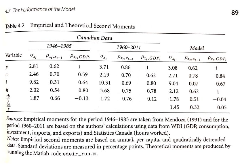
For your convenience, scans of Tables 4.1 and 4.2 from Uribe and Schmitt-Grohé (2017) are reproduced at the end of
this document in Figures 1 and 2.
PART I
1 Data Preparation
Complete the following data preparations and comparisons to the benchmark open economy.
For this question, feel free to use a software package of your choice, including Excel, Stata or Matlab. For sample code
in Matlab or Stata, please see the files at StudyNet (Canvas) or econ.ucsd.edu/muendler/teach/21s/8270.
The deliverable product for this question has five components: a report of a single number (the Swiss mean capital
share), a report of higher-order moments for statistics in three country-specific tables, a written discussion of results and
their comparisons, a copy of the prepared data, and a copy of the Matlab code (or Stata code, Excel macro/spreadsheet, or
the like).
1. Obtain World Development Indicators (WDI) data for all available countries over the period 1985–2019 and the
following time series, at the annual frequency:
• NY.GDP.PCAP.KN: Real GDP per capita (constant LCU) yt ,
• NE.CON.PRVT.ZS: Households and NPISHs final consumption expenditure (percent of GDP) c̈t and compute
consumption expenditure per capita ct = c̈t yt /100,
• NE.GDI.TOTL.ZS: Gross capital formation (percent of GDP) ϊt and compute investment per capita it =
ϊt yt /100,
• NE.CON.GOVT.ZS: General government final consumption expenditure (percent of GDP) g̈t and compute gov-
ernment expenditure per capita gt = g̈t yt /100,
1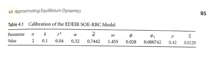
• NE.IMP.GNFS.ZS: Imports of goods and services (percent of GDP) m̈t and compute imports per capita mt =
        m̈t yt /100,
      • NE.EXP.GNFS.ZS: Exports of goods and services (percent of GDP) ẍt and compute exports per capita xt =
        ẍt yt /100,
      • BN.CAB.XOKA.GD.ZS: Current account balance (percent of GDP) ca  ¨ t and compute the current account per
        capita cat = ca
                      ¨ t yt /100.
   You should visit the WDI download portal datacatalog.worldbank.org/dataset/world-development-indicators. A csv
   (comma separated values) format might be most useful, as it is understood by most statistical and computational
   software packages.
2. Obtain hours worked per capita ht data for all available countries over the period 1985–2019 from the Conference
   Board’s Total Economy Database www.conference-board.org/data/economydatabase, using the series TED1, 1950–
   2019. (If you prefer not to set up an account, please download the data from StudyNet (Canvas).) A csv (comma
   separated values) format might be most useful. Note that ht is total hours worked per capita, not per worker. Merge
   the time series for ht with those from the World Development Indicators (WDI) by country and year. As the country
   variable for the merge, use the ISO-3 code.
3. Drop all countries for which at least one variable has less than three non-missing values in the period 1985–2019.
4. For Switzerland, obtain the capital share in national income for the period 1995–2019 from the Swiss Federal Sta-
   tistical Office www.bfs.admin.ch/bfs/en/home/statistics. For this purpose, use Swiss gross domestic product under
   the income approach and compute the annual share of compensation of employees (D.1) in gross domestic product
   (B.1∗b). Note that the capital share is one less the labor share in national income. Report the unweighted mean
   capital share in national income over the full period 1995–2019.
5. Detrend the time series from items 1 and 2. See sample codes data prep and detrend Q1.m (Matlab) and/or data -
   prep and detrend Q1.do (Stata).
      • For real output yt , consumption ct , investment it , government spending gt and hours worked ht per capita,
        detrend (separately) the natural logarithms using a log-quadratic trend as in section 1.1 of the Uribe and Schmitt-
        Grohé (2017) textbook. For example, for log real output per capita ln yt , fit the ordinary-least squares regression
        ln yt = β0 + β1 (t − 1985) + β2 (t − 1985)2 + ln ytc , where the residual ln ytc is called the cyclical component
        and the fitted part is called the secular (or trend) component ln yts . Store the cyclical component of all variables.
      • For the trade-balance-to-output ratio tbt /yt = (xt − mt )/yt and the current-account-to-output ratio cat /yt
        detrend (separately) the levels using a quadratic trend as in section 1.1 of the Uribe and Schmitt-Grohé (2017)
        textbook. For example, for the current-account-to-output ratio cat /yt , fit the ordinary-least squares regression
        cat /yt = β0 + β1 (t − 1985) + β2 (t − 1985)2 + t , where the residual is the cyclical component. Store the
        cyclical component of all variables.
      • For the level of the trade balance per capita tbt = xt −mt and the level of the current account cat per capita, first
        divide them by the secular component of real output per capita exp{ln yts }, and then detrend (separately) the
        levels using a quadratic trend as in section 1.1 of the Uribe and Schmitt-Grohé (2017) textbook. For example,
        for the trade balance per capita tbt , fit the ordinary-least squares regression tbt / exp{ln yts } = β0 + β1 (t −
        1985) + β2 (t − 1985)2 + t , where the residual is the cyclical component. Store the cyclical component of all
        variables.
6. Compute the standard deviation, the serial correlation coefficient, and the correlation coefficient with the cyclical
   component of GDP per capita (ln ytc ) for (i) Canada, (ii) Switzerland and (iii) either one poor country or one emerging
   market for the period 1985–2019 using the cyclical components of the detrended variables from item 5. Report the
   results in three separate tables, one per country.
7. Compare the results from item 6 for (i)–(iii) with each other (“cross-sectional” analysis), and compare the results
   for country (i) over the period 1985–2019 to those reported for Canada for the period 1960–2011 in the Uribe and
   Schmitt-Grohé (2017) textbook, middle panel of Table 4.2, and those in the Mendoza (1991) benchmark paper, left
   panel of Table 4.2 in the textbook (“panel” analysis). What is the ranking of volatilities in countries (i)–(iii) during
   our period?

                                                            2
PART II
2 Decentralized Economy and Planner Problem
Using the first-order conditions and equilibrium relationship from the decentralized version of the EDEIR model, derive the
planner’s version of the model as presented in the Uribe and Schmitt-Grohé (2017) textbook. For all derivations, assume
for simplicity that households and firms have perfect foresight, and omit the expectations operator.
The deliverable product for this question has one component: a written derivation of the planner’s version of the model
from the decentralized economy version.
For this question, recall the following conventions on notation:
• Elasticity of intertemporal substitution: σ̄ in decentralized economy (lecture notes) and Obstfeld and Rogoff (1996)
but σ ≡ 1/σ̄ in planner problem of Uribe and Schmitt-Grohé (2017);
• Net foreign wealth bt in decentralized economy (lecture notes) and Obstfeld and Rogoff (1996) but dt−1 ≡ −bt in
planner problem of Uribe and Schmitt-Grohé (2017);
• Interest rate quoted today for returns tomorrow rt in decentralized economy (lecture notes) and Obstfeld and Rogoff
(1996) but rt−1 = (r∗ + p(dt−1 )) in planner problem of Uribe and Schmitt-Grohé (2017);
• Firm’s maximized (ex-dividend) value vt in decentralized economy (lecture notes) and Obstfeld and Rogoff (1996)
but pst in planner problem of Uribe and Schmitt-Grohé (2017);
• Equity shares θt in decentralized economy (lecture notes) but st in planner problem of Uribe and Schmitt-Grohé
(2017);
• Dividend div t = ut kt −it − φ2 (kt+1−kt )2 in decentralized economy (lecture notes) but πt in Uribe and Schmitt-Grohé
(2017).
1. For the representative household’s dynamic programming problem, explain the Bellman function
U (bs , θs ) = max [u(cs , hs ) + βU (bs+1 , θs+1 )]
bs+1 ,θs+1 ,hs
under the intertemporal budget constraint cs = (1 + rs )bs − bs+1 − vs (θs+1 − θs ) + div s θs + ws hs .
2. Derive the first-order conditions, including the one for labor supply, and state the transversality conditions for global
bond holdings (net foreign wealth) and domestic equity. Why can the transversality conditions be considered first-
order conditions in the decentralized economy?
3. Assume complete home bias in equity so that θt = 1 in equilibrium. Derive the Euler equation for consumption
(global bond holdings) and the intertemporal optimality condition for equity holdings from the preceding first-order
conditions.
4. Define λt ≡ uc (cs , hs ). From the above results, derive the first-order conditions (4.5), (4.7) and (4.8) as well as the
equilibrium conditions (4.17) and (4.19) for the planner’s problem in Uribe and Schmitt-Grohé (2017, Ch. 4).
5. In the setup of the decentralized economy, there are two production sectors. In one sector, firms produce and rent
out capital goods to other producers. Denote the rental rate for a unit of capital with ut . For a capital accumulation
function ks+1 = (1−δ)ks + is and under quadratic adjustment costs φ2 (ks+1 − ks )2 , the Bellman equation can be
written as
φ 1
V (ks ) = max us ks − is − (ks+1 − ks )2 + V (ks+1 ) .
ks+1 2 1 + rs
Explain why.
6. In the other production sector, final-goods manufacturers combine capital and labor under a Cobb-Douglas production
function with capital intensity α and a Hicks-neutral productivity factor At . Derive the final-goods manufacturer’s
first-order conditions for capital and labor demand.
37. Derive the capital producing firms’ dividends in terms of returns on capital at the final-goods manufacturers.
8. Derive the capital providing firms’ intertemporal optimality condition. With this result and λt ≡ uc (cs , hs ), derive
the first-order condition (4.10) as well as the equilibrium condition (4.18) for the planner’s problem in Uribe and
Schmitt-Grohé (2017, Ch. 4), using the specific functional form for quadratic adjustment costs from above.
9. Use the final-goods manufacturers’ first-order conditions together with the household’s first-order condition for opti-
mal labor supply to derive the first-order conditions (4.9) and (4.11) for the planner’s problem in Uribe and Schmitt-
Grohé (2017, Ch. 4), with the specific functional form for Cobb-Douglas production but without any parametric
assumption on optimal labor supply.
10. Use the expression for optimal dividends from above in the intertemporal budget constraint cs = (1 + rs )bs − bs+1 −
vs (θs+1 − θs ) + div s θs + ws hs together with Euler’s Theorem to derive the equilibrium conditions (4.16), (4.20),
and (4.21) for the planner’s problem in Uribe and Schmitt-Grohé (2017, Ch. 4).
3 Simulating the EDEIR model for Canada
Simulate the EDEIR model for the Canadian economy, using the calibrated values from the Uribe and Schmitt-Grohé (2017)
textbook.
For this question use Matlab. Most economists would arguably complete this simulation step in Matlab. For sample code
in Matlab, similar to that at www.columbia.edu/ mu2166/book by Uribe and Schmitt-Grohé, please see the files at StudyNet
(Canvas) or econ.ucsd.edu/muendler/teach/21s/8270. Note that you do not need to reprogram or adjust any Matlab file for
this question. Matlab files with names that end in “ Q3.m” are used only in question 3.
The deliverable product for this question has one component: a written discussion of the ability of the model to explain
observed business cycle patterns in Canada.
1. This step is already completed in the code but still listed for completeness. Set the following parameters without
a relationship to specific country data for 1985–2019, following Mendoza (1991) (also reported in Table 4.1 of the
Uribe and Schmitt-Grohé (2017) textbook):
• the parameter σ (the inverse of the intertemporal elasticity of substitution),
• the depreciation rate δ,
• the world interest rate r∗ ,
• and the subjective discount factor β = 1/(1 + r∗ ).
2. This step is already completed in the code but still listed for completeness. Set the following parameters as in Table 4.1
of the Uribe and Schmitt-Grohé (2017) textbook:
• the capital elasticity α of the Cobb-Douglas production function,
• the parameter ω, which determines the wage elasticity of labor supply 1/(ω − 1),
• the parameter φ, which governs capital adjustment costs,
• the parameter ψ, which regulates the sensitivity of the real interest rate to a country’s net wealth,
• the persistence of the technology shock ρ, and
• the volatility of the technology shock η,
For this purpose, approximate the equilibrium dynamics up to first order using the Matlab procedure from sections 4.5
and 4.6 of the Uribe and Schmitt-Grohé (2017) textbook.
3. Compute the model-implied (theoretical) second moments as in the Uribe and Schmitt-Grohé (2017) textbook, right-
most panel of Table 4.2. Comment on the ability of the model to explain observed business cycle patterns in Canada
between 1985 and 2019, using the standard deviation, the serial correlation coefficient, and the correlation coefficient
with the cyclical component of GDP per capita (ln ytc ) for Canada from item 5 in question 1 above.
44 Calibrating the EDEIR model to Switzerland
Calibrate the EDEIR model of the Uribe and Schmitt-Grohé (2017) textbook to the Swiss economy.
For this question use Matlab. For sample code in Matlab beyond the textbook-provided code (a loop over the steady-
state simulation), please see the files at StudyNet (Canvas) or econ.ucsd.edu/muendler/teach/21s/8270. Note that you do
need to reprogram or adjust the Matlab files with names that end in “ Q4.m”.
The deliverable product for this question has three components: a copy of your edited Matlab code, a report of five
calibrated parameter values, and a written discussion of the ability of the model to explain observed business cycle patterns
in Switzerland.
1. This step is already completed in the code but still listed for completeness. Set the following parameters without a
relationship to the Swiss data for 1985–2019, following Mendoza (1991) (also reported in Table 4.1 of the Uribe and
Schmitt-Grohé (2017) textbook):
• the parameter σ (the inverse of the intertemporal elasticity of substitution),
• the depreciation rate δ,
• the world interest rate r∗ ,
• and the subjective discount factor β = 1/(1 + r∗ ).
2. Set the following parameters to match the first moments of the Swiss data:
• the capital elasticity of the production α to one less the average labor share in national income for Switzerland
for the period 1995–2019,
• the composite parameter b̄/y ≡ −d/y ¯ so that −b̄/y = d/y ¯ = (tb/y)/r∗ , where tb/y is the raw ratio (not
∗
detrended) from the Swiss data for 1985–2019, r is as calibrated above, and steady-state output will then be
determined by the model’s parameters (y = [(1 − α)καω ]1/(ω−1) and κ = [α/(r∗ + δ)]1/(1−α) ), similar to the
procedure in section 4.5 of the Uribe and Schmitt-Grohé (2017) textbook.
3. From your answer to item 5 in question 1 above, use the following seven higher moments of the Swiss data for
1985–2019 as target values for calibration:
• the standard deviation of (the cyclical component of) hours worked ht ,
• the standard deviation of (the cyclical component of) investment it ,
• the serial correlation of (the cyclical component of) investment it ,
• the standard deviation of (the cyclical component of) the trade-balance-to-output ratio tbt /yt = (xt − mt )/yt ,
• the serial correlation of (the cyclical component of) the trade-balance-to-output ratio tbt /yt = (xt − mt )/yt ,
• the standard deviation of (the cyclical component of) output yt , and
• the serial correlation of (the cyclical component of) output yt .
Adjust the Matlab code that loops over the steady-state simulations and minimizes the deviation of the model-
produced seven moments from the empirical seven moments above. The Matlab iteration routine sets and resets
the following five parameters to match the preceding seven higher moments:
• the parameter ω, which determines the wage elasticity of labor supply 1/(ω − 1),
• the parameter φ, which governs capital adjustment costs,
• the parameter ψ. which regulates the sensitivity of the real interest rate to a country’s net wealth,
• the persistence of the technology shock ρ, and
• the volatility of the technology shock η.
For the steady-state computations, approximate the equilibrium dynamics up to first order using the Matlab procedure
described in sections 4.5 and 4.6 of the Uribe and Schmitt-Grohé (2017) textbook but feed the calibrated values for
the Swiss economy into each iterative call of the steady-state computation. As starting values for the Swiss economy,
use the Canada-calibrated parameters as in Table 4.1 of the Uribe and Schmitt-Grohé (2017) textbook.
54. Report the calibrated parameter values for ω, φ, ψ, ρ, and η.
5. Compute the model-implied (theoretical) second moments as in the Uribe and Schmitt-Grohé (2017) textbook, right-
most panel of Table 4.2, but now for the calibration to Switzerland.
6. Comment on the ability of the model to explain observed business cycle patterns in Switzerland between 1985 and
2019.
5 Sensitivity of Calibrated Parameters to Target Moments
Calibrate the EDEIR model of the Uribe and Schmitt-Grohé (2017) textbook to the Swiss economy with two alterations, to
assess the sensitivity of calibrated parameters to target moments.
Reuse your Matlab code from question 4 and alter the target moments as stated below.
The deliverable product for this question has three components: a copy of your edited Matlab code, a report of five
calibrated parameter values, and a written discussion of the sensitivity of the calibrated parameters to alterations of the
moments.
1. From your seven higher moments of the Swiss data for 1985–2019 in item 3 of question 4 above, raise the standard
deviation of (the cyclical component of) hours worked ht to 140 percent of its actual value in the data. As in item 3
of question 4 above, launch the Matlab iteration routine to find the following five parameters under the new target: ω,
φ, ψ, ρ, and η. Report the calibrated parameter values and explain why they differ from the prior calibration.
2. From your seven higher moments of the Swiss data for 1985–2019 in item 3 of question 4 above, reduce the standard
deviation of (the cyclical component of) investment it to half its actual value in the data. As in item 3 of question 4
above, launch the Matlab iteration routine to find the following five parameters under the new target: ω, φ, ψ, ρ, and
η. Report the calibrated parameter values and explain why they differ from the prior calibration.
References
Mendoza, Enrique G, “Real Business Cycles in a Small Open Economy,” American Economic Review, 1991, 81 (4), 797–818.
Obstfeld, Maurice and Kenneth Rogoff, Foundations of international macroeconomics, Mass and London: MIT Press, 1996.
Uribe, Martin and Stephanie Schmitt-Grohé, Open Economy Macroeconomics, Princeton and Oxford: Princeton University Press,
2017.
6Reproduction of Textbook Tables
Figure 1: Table 4.1 from Uribe and Schmitt-Grohé (2017, p. 85)
Figure 2: Table 4.2 from Uribe and Schmitt-Grohé (2017, p. 89)
7You can also read