Air Quality Index Monitoring Based on Profile-MEWMA Control Chart - IOPscience

Journal of Physics: Conference Series

PAPER • OPEN ACCESS

Air Quality Index Monitoring Based on Profile-MEWMA Control Chart
To cite this article: Yingjie Liu and Xuemin Zi 2021 J. Phys.: Conf. Ser. 1955 012051

View the article online for updates and enhancements.

 This content was downloaded from IP address 46.4.80.155 on 13/08/2021 at 06:58

ISBDAS 2021 IOP Publishing
Journal of Physics: Conference Series 1955 (2021) 012051 doi:10.1088/1742-6596/1955/1/012051

Air Quality Index Monitoring Based on Profile-MEWMA
Control Chart

 Yingjie Liu1*, Xuemin Zi2
 1*
 School of science, Tianjin University of Technology and Education, Tianjin, Tianjin,
 300222, China
 2
 School of science, Tianjin University of Technology and Education, Tianjin, Tianjin,
 300222, China
 *
 E-mail: rkchp@zhobk.cn

 Abstract. At present, due to the rapid development of domestic economy, the environmental
 pollution problems are becoming increasingly serious, especially the pollution problems such as
 PM2.5 and PM10 caused by industrial emissions and waste gas pollution are most urgent. The
 general linear profile model and multivariate exponential weighted moving average control chart
 (MEWMA) is designed to perform monitoring and evaluating the air quality index (AQI) in
 Tianjin, so as to provide some statistical information for the relevant departments. Six main
 pollutants , , 10, 2.5, , in Tianjin were collected which taken as factors
 affecting AQI under consider establish a general linear profile model where AQI was taken as
 the response variable. The coefficients of the model are monitoring by an MEWMA control chart.

1. Introduction
In the past, there are many different ways in which change monitoring can be performed. The functional
relationship between a response variable and one or more predictor variables used to describe the quality
of a process called a profile. Some general issues about profile monitoring profile monitoring arises in
Woodall et al. (2004) [1]. For the purpose of calibration that has been considered apply profile model in
the relevant literatures, for example, Mestek et al. (1994) [2], Kang and Albin (2000) [3], Ajmani (2003)
[4] and Mahmoud and Woodall (2004) [5].
 All of the above-mentioned applications can be separated into Phase I control and Phase II
monitoring. In-control values of the process parameters were estimated in phase I which can evaluate
the stability of the process and in order to quickly and exactly detect any shift in the Phase II process
can be considered to monitor future observations. In this paper, we introduce establishing a practical
control chart based on the profile model which are a large class of statistical models for relating
responses to linear combinations of predictor variables to monitor the AQI in Tianjin. Basically, the
same algorithms can be used to estimate, inference, and evaluate the adequacy of the model for all
general linear models (GLMs) which provides a general theoretical framework for many common
statistical models and simplifies the implementation of these models in statistical software. In fact, most
of the studies mentioned above can be regarded as special cases of the GLM profile. A GLM method
based on log-linear model for the first time proposed Qiu (2008) [6] who suggested a methodology relied
on the log-linear mode for estimating the in-control multivariate measurement distribution and then used
a multivariate CUSUM procedure for detecting shifts in the location parameter vector of the
measurement distribution for phase II when a set of in-control data is available. Yeh et al. (2009) [7]

 Content from this work may be used under the terms of the Creative Commons Attribution 3.0 licence. Any further distribution
 of this work must maintain attribution to the author(s) and the title of the work, journal citation and DOI.
Published under licence by IOP Publishing Ltd 1

ISBDAS 2021 IOP Publishing
Journal of Physics: Conference Series 1955 (2021) 012051 doi:10.1088/1742-6596/1955/1/012051

performed several Hotelling charts so that monitoring the parameters in phase I used a logistic
regression. In this study, they used a real data from aircraft industry in which a binary regression model
was designed between the total number of alloy fasteners that failed check at a certain load and loading
strength which regard as response variable and predictor variable, respectively. Furthermore studied
about a control chart in this problem to phase II process were proposed for the parameters of a logistic
regression model by integrating a likelihood-ratio test and an EWMA scheme described by Shang et al.
(2011) [8].
 EWMA has been widely concerned and studied by scholars since as soon as it was first proposed by
Robert (1959) and developed rapidly in the following years. Lucas and Saccucci (1990) [9] showed that
the EWMA control chart is more effective for small shift when the (weight parameter) is smaller, and
more valid for large shift when the is larger. This method was widely used in industrial production
over the next few years, Lowry (1992) [10] introduced the multi-EWMA series (MEWMA) which filled
the gap in the multivariate control chart. This paper adopts the combination of generalized linear profile
model and MEWMA control chart to monitoring and evaluating the AQI in Tianjin, which has certain
practical significance.

2. Methodology

2.1. Profile model
Assume the observed value , are obtained at the sample point, where is an dimensional
response variable and is an matrix. When the process is in-control, we have profile
model as follows:
 (1)
where , ,…, , is a multivariate normal random variable defined as Ε 
0 , . In the above equation, 1, ∗ , where ∗ and 1 are orthogonal, 1 represents the
1-dimension vector in which the elements are all 1. In our case, denotes as and ∗ is regard as 
which is supposed to be the same for different in the application of profile. There are q+1 coefficients
and standard deviations that need to be monitored simultaneously for a general linear profile model
[11]. Define the following formula:
 / (2)
 / ; (3)
where
 (4)
 (5)
 In the above equation, ⋅ is the inverse normal distribution, ⋅; is the distribution function
of the Chi Square distribution with degree of freedom. Such a change has the following excellent
properties:
1) is independent of the sample size when the process is in-control which is convenient for our
design.
2) Making the control chart sensitive to a reduction in the variance of the profile because of the
distribution of is symmetric.
 Define , is a multivariate normal random variable with the Ε 0 and
covariance matrix is Σ 0 while the process is in-control.
 0 1

2.2. MEWMA control chart
A monitoring method based on a sequence of MEWMA control charts can be defined as follows:

 2

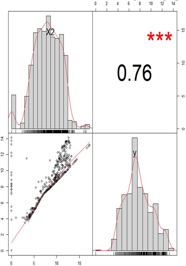
ISBDAS 2021 IOP Publishing
Journal of Physics: Conference Series 1955 (2021) 012051 doi:10.1088/1742-6596/1955/1/012051

 1 , 1,2. . ., (6)
in which 0 is the initial vector of p+1 dimension, 0    1 is the weight parameter, and the
MEWMA control chart alarms when
 (7)
where the UCL is the control limit which leads to an estimate given by the in control average running
length ) that obtained through the quantile of in-control process statistics after determining other
parameters. Generally, the larger is sensitive to large shift, while the smaller is favor to small shift.
The coefficients obtained by general linear profile of the model were monitored using a MEWMA
control chart.

3. Real-Data
To further illustrate the performance of the proposed control chart, we consider provide the guideline
on how to apply the Profile-MEWMA control chart to real data and show the performances of
monitoring efficiency. The parameters of the profile model are monitoring by using MEWMA control
chart while a profile model is constructed by least square calculation to estimate the controlled
coefficients. For this we sequentially collect six indicators and AQI from January 1, 2019 to December
31, 2020 in Tianjin while AQI below 100 is set as in-control data. In addition, the data from 0:00 on
January 1, 2021 to 24:00 on January 31, 2021 are collected by the hour as monitoring data where the
 2.5, 10, , , , are taken as the factors affecting AQI (regardless of their interaction).
 To simplified the notations, we can write:
 , , , , , 
let X is a vector the entries represent the concentrations of 2.5, 10, , , , respectively
and Y denotes AQI. The estimations of the coefficients of the profile model are given in Table 1 which
gives the coefficient estimates, standard error, p-value, t-value and significance for the six variables that
demonstrates there is no significant correlation between and AQI. Five factors are taken as
explanatory variables by using step regression methods to reestimate in-control coefficients.
 Table 2 shows numerical characteristics of 2.5, 10, , , data in Tianjin. From Table
2, it seems, that a simple summary of the data has been achieved which makes it easy to see what
conclusions can be drawn. According to the correlation analysis shows that 2.5 and 10 are
important factors affecting the AQI (as shown in Figure 1). And the three variables with the largest
variances are 10, , 2.5 in order which indicating that those data fluctuates greatly, while the
distributions of these three variables are all have the characteristics of sharp peaks and thick tails,
therefore the distribution of , and is close to the normal distribution based on the kurtosis
values. Each skewness of all variables is greater than 0 that reflects the distribution of data is skewed to
the right.
 Table 1: Least square fitting results.
 Time Estimate Std. Error t value Pr (>|t|) Significance
 Intercept 4.28239 1.23149 3.477 0.000532 ***
 X1 0.48239 0.03125 15.436

ISBDAS 2021 IOP Publishing
Journal of Physics: Conference Series 1955 (2021) 012051 doi:10.1088/1742-6596/1955/1/012051

plot and the fitting curve between PM2.5, PM10 and AQI respectively. According to the figures we
notice that both PM2.5 and PM10 have significant effects on AQI that showed a strong positive linear
correlation. Intuitively higher concentrations of PM2.5 and PM10 lead to the higher AQI value, that is,
the worse air quality. Recall from Section 2 some parameters can be calculated in which 9.171,
 4.24,0.48,0.37,5.07,0.06,0.19 , 148785.8 and 155794.8 under 0.1 and
 0.2 from the in-control data. A more complete outline of the in-control limit algorithm is detailed
in Table 3. The results for statistic U are summarized in Table 4. Figure 2 and Figure 3 show the plot
of U and real data of AQI respectively.
 Table 2：Characteristics of PM 2.5, PM 10, CO, NO2,O3 data in Tianjin.

 quantile quantile
 Variable min median mean max variance skewness kurtosis
 (0.25) (0.75)
 AQI 15 49.75 76 86.0579 118 334 2562.127 1.0544 1.4091
 PM2.5 3 20 45 54.4748 82.25 186 1637.358 0.82699 0.0394
 PM10 3 46 83 90.9033 120 447 3829.03 1.6467 5.3629
 CO 4 0.6 0.9 0.989942 1.3 2.8 0.2348153 0.4830 -0.3735
 NO2 0.2 25 46 44.6427 62 112 525.7761 0.1234 -0.6530
 O3 1 13 34 36.7557 57 128 636.7318 0.5642 -0.3716

 We report the following performance measures by combining the real AQI in Figure 2 with the results
in Figure 3. The dashed line is the in-control limit. For 0.1 and 0.2 it can be seen that the
control chart sent out an alarm signal on the January 31, 2021 from Figure 3 (a) and (b) which indicating
the air quality drop to a lower level that is consistent with the actual situation. The result means that the
monitoring model in this paper has practical significance and can be applied to air quality monitoring.
By comparing the real situation in Figure 3 (a) and (b) from January 15, 2021 to January 19, 2021, it
also shows that when the data shift occurs, the smaller has a better effect on monitoring change points.

 Figure1：Correlation diagram of PM2.5 concentration, PM10 concentration and AQI.

 4

ISBDAS 2021 IOP Publishing
Journal of Physics: Conference Series 1955 (2021) 012051 doi:10.1088/1742-6596/1955/1/012051

 Figure2：Real AQI in January 2021 in Tianjin.

 Table 3: In-control limit algorithm
Algorithm1: Outline of the in-control limit

Inputs: Observed statistic , , initial W=0
Outputs: U, in-control limit UCL
 Estimated in-control coefficient by using the least square estimation based on observed statistic
 Obtain in-control coefficient, standard deviation
 Generate 24000 in-control data, each 24 data is used as a profile sample
for i ∈ {1:1000}
 Update 
 Re-estimate in-control coefficients using least squares estimation.
end for Record each coefficient
for j ∈ {1:1000}
 Calculate statistic , according to formula (2), (3), (6)
 Calculate and store according to formula (7)
end for
Return Calculate the quantile of as the in-control limit UCL, 

 Table 4: The calculation result of statistic
 U U U U U U U U
 Time Time Time Time
 （λ=0.1） （ λ= 0.2） （λ=0.1） （ λ= 0.2） （λ=0.1） （ λ= 0.2） （λ=0.1） （ λ= 0.2）
 01-01 2211 8847 01-09 53331 92597 01-17 138869 174100 01-25 236519 337841
 01-02 10301 37484 01-10 62924 107003 01-18 140367 170160 01-26 242615 332834
 01-03 25222 84037 01-11 64863 102013 01-19 143926 172652 01-27 243435 318162
 01-04 35609 105003 01-12 166591 380337 01-20 147139 172652 01-28 253260 323162

 5

ISBDAS 2021 IOP Publishing
Journal of Physics: Conference Series 1955 (2021) 012051 doi:10.1088/1742-6596/1955/1/012051

 01-05 46112 122974 01-13 145148 268852 01-21 167999 215803 01-29 258149 318203
 01-06 46070 105684 01-14 153602 262723 01-22 176017 226705 01-30 261895 314603
 01-07 57127 125184 01-15 159964 254598 01-23 188778 248252 01-31 256125 291004
 01-08 62664 126103 01-16 143183 194474 01-24 201816 268604

 Figure 3：Plot of real data cases results.

4. Conclusion
In this article, we use a general theoretical framework for monitoring the changes in parameters and
standard deviation for the profile models in the process. In fact, the profile model is considered to
describe the relationship between response variables and one or more predictors. Based on this
theoretical, we establish a linear profile model with AQI as the response variable and five major factors
affecting air quality as the predictive variables that combine with MEWMA control chart to monitoring
the air quality in Tianjin. The results show that the model can accurately detect the change of AQI and
reflect the change of air quality, which has a certain guiding significance for air quality monitoring.
Next, we can further study extend the method when consider the interaction between influencing factors,
so as to achieve better monitoring effect.

Acknowledgments
This paper was supported by the NNSF of China, grants No. 11771d332 and 11771220.

References
[1] Woodall, W. H., Spitzner, D. J., Montgomery, D. C., and Gupta, S. (2004). Using Control Charts
 to Monitor Process and Product Quality Profiles. Journal of Quality Technology 36:309– 320.
[2] Mestek, O., Pavlik, J., and Suchánek, M. (1994). Multivariate Control Charts: Control Charts for
 Calibration Curves. Fresenius’ Journal of Analytical Chemistry 350:344–351.
[3] Kang, L. and Albin, S. L. (2000). On-Line Monitoring When the Process Yields a Linear Profile.
 Journal of Quality Technology 32:418–426.

 6

ISBDAS 2021 IOP Publishing
Journal of Physics: Conference Series 1955 (2021) 012051 doi:10.1088/1742-6596/1955/1/012051

[4] Ajmani, V. (2003). Using EWMA Control Charts to Monitor Linear Relationships in
 Semiconductor Manufacturing. Joint Statistical Meetings, San Francisco, CA.
[5] Mahmoud, M. A. and Woodall, W. H. (2004). Phase I Analysis of Linear Profiles with Calibration
 Applications. Technometrics 46:380–391.
[6] Qiu, P. (2008). Distribution-free multivariate process control based on log-linear modeling. IIE
 Transactions 40:664–677.
[7] Yeh, A. B., Huwang, L., and Li, Y. M. (2009). Profile Monitoring for a Binary Response. IIE
 Transactions 41:931–941
[8] Shang, Y., Tsung, F., and Zou, C. (2011). Phase-II Profile Monitoring with Binary Data and
 Random Predictors. Journal of Quality Technology 43:196-208.
[9] Lucas, J. M. and Saccucci, M. S. (1990). Exponentially Weighted Moving Average Control Scheme
 Properties and Enhancements. Technometrics 32:1–29.
[10] Lowry, C. A., Woodall, W. H., Champ, C. W., and Rigdon, S. E. (1992). Multivariate Exponentially
 Weighted Moving Average Control Chart. Technometrics 34:46–53.
[11] Kim, K., Mahmoud, M. A., and Woodall, W. H. (2003). On the Monitoring of Linear Profiles.
 Journal of Quality Technology 35:317-328.

 7