P&S Heterogeneous Systems - Parallel Patterns: Graph Search Dr. Juan Gómez Luna Prof. Onur Mutlu - ETH Zürich
←
→
Page content transcription
If your browser does not render page correctly, please read the page content below
P&S Heterogeneous Systems
Parallel Patterns: Graph Search

        Dr. Juan Gómez Luna
          Prof. Onur Mutlu
             ETH Zürich
            Spring 2022
            24 May 2022
Parallel Patterns

Reduction Operation
n    A reduction operation reduces a set of values to a single
     value
     q    Sum, Product, Minimum, Maximum are examples

n    Properties of reduction
     q    Associativity
     q    Commutativity
     q    Identity value

n    Reduction is a key primitive for parallel computing
     q    E.g., MapReduce programming model

Dean and Ghemawat, “MapReduce: Simplified Data Processing of Large Clusters,” OSDI 2004   3
Divergence-Free Mapping (I)
      n      All active threads belong to the same warp
                 Thread 0 Thread 1 Thread 2   …                Thread 14 Thread 15

                      0         1     2           3   …   13      14       15        16   17   18   19

             1 0+16                                                     15+31

             2
iterations

             3

     Slide credit: Hwu & Kirk                                                                            4
Divergence-Free Mapping (II)
n   Program with high SIMD utilization
__shared__ float partialSum[]

unsigned int t = threadIdx.x;

for(int stride = blockDim.x; stride > 0;    stride >> 1){

    __syncthreads();

    if (t < stride)
      partialSum[t] += partialSum[t + stride];

}
                                                  A[0]   Warp
                                                          A[1] 0   Warp 1   Warp 2   Warp 3 A[N-1]

                                    stride = 16

    Warp utilization                stride = 8
    is maximized
                                    stride = 4

                                                                                      5
Histogram Computation
n     Histogram is a frequently used computation for reducing
      the dimensionality and extracting notable features and
      patterns from large data sets
      q     Feature extraction for object recognition in images
      q     Fraud detection in credit card transactions
      q     Correlating heavenly object movements in astrophysics
      q     …
n     Basic histograms - for each element in the data set, use the
      value to identify a “bin” to increment
      q     Divide possible input value range into “bins”
      q     Associate a counter to each bin
      q     For each input element, examine its value and determine the
            bin it falls into and increment the counter for that bin

                                                                      6
Slide credit: Hwu & Kirk
Parallel Histogram Computation: Iteration 2
n       All threads move to the next section of the input
        q   Each thread moves to element threadID + #threads

I       _ C     A    L   C   U   L    A   T     E   _   A    _ H       I   S   T   O   G      R       A       M

              Thread 0               Thread 1               Thread 2               Thread 3

                         We need to use atomic operations

    1   1        2
                 1                         1            2                                         1
    _   A   B    C D     E   F   G H      I     J   K   L M N O            P   Q R     S   T      U           V…
                                                                                                          7
Histogram Privatization
n   Privatization: Per-block sub-histograms in shared memory
    q   Threads use atomic operations in shared memory
                                                   Block 0             Block 1

                                                   Block 2             Block 3

                                                   Block 0             Block 1

                                                   Block 2             Block 3

                                                   Block 0             Block 1

                                                   Block 2             Block 3

                                                   Block 0             Block 1

                                                   Block 2             Block 3

                    Block 0’s sub-histo Block 1’s sub-histo       Block 2’s sub-histo      Block 3’s sub-histo
    Shared memory    b0   b1   b2   b3   b0   b1     b2      b3    b0    b1      b2   b3   b0   b1   b2   b3

                                                                                           Parallel reduction

                                                    b0       b1   b2    b3        Global memory

                                                     Final histogram

                                                                                                                 8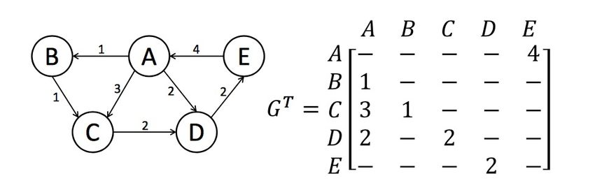
Convolution Applications
n    Convolution is a widely-used operation in signal processing,
     image processing, video processing, and computer vision

n    Convolution applies a filter or mask or kernel* on each
     element of the input (e.g., a signal, an image, a frame) to
     obtain a new value, which is a weighted sum of a set of
     neighboring input elements
     q     Smoothing, sharpening, or blurring an image
     q     Finding edges in an image
     q     Removing noise, etc.

n    Applications in machine learning and artificial intelligence
     q     Convolutional Neural Networks (CNN or ConvNets)
* The term “kernel” may create confusion in the context of GPUs (recall a CUDA/GPU kernel is a function executed by a GPU)   9
1D Convolution Example
n Commonly used for audio processing
n Mask size is usually an odd number of elements for
symmetry (5 in this example)
n Calculation of P[2]:
N N[0] N[1] N[2] N[3] N[4] N[5] N[6] P P[0] P[1] P[2] P[3] P[4] P[5] P[6]
1 2 3 4 5 6 7 3 8 57 16 15 3 3
Sum
M M[0] M[1] M[2] M[3] M[4]
3 4 5 4 3 3 8 15 16 15
Partial products
Slide credit: Hwu & Kirk 10Another Example of 2D Convolution
Input Output
Layer CNN Y Layer
X
1 2 3 4 5 6 7 filter 1 2 3 4 5
W 2 3 4 5 6
2 3 4 5 6 7 8 1 2 3 2 1
2 3 4 3 2 3 4 321 6 7
3 4 5 6 7 8 9
3 4 5 4 3 4 5 6 7 8
4 5 6 7 8 5 6 2 3 4 3 2
1 2 3 2 1 5 6 7 8 5
5 6 7 8 5 6 7
6 7 8 9 0 1 2
7 8 9 0 1 2 3
1 4 9 8 5
Sum
4 9 16 15 12
Partial products
9 16 25 24 21
8 15 24 21 16
5 12 21 16 5
Slide credit: Hwu & Kirk 11Implementing a Convolutional Layer
with Matrix Multiplication
12 18 10 20 Output
Features
13 22 15 22 Y
Convolution
1 1 1 1 0 1 1 0 2 1 1 2
Filters
2 2 1 1 1 0 0 1 2 1 2 0
W
1 2 0 0 2 1 1 2 1 Input
1 1 3 0 1 2 0 1 3 Features
0 2 2 1 1 0 3 3 2 X
1 1 2 2 1 1 1 1 0 1 1 0 1 2 1 1 12 18 13 22
1 0 0 1 2 1 2 1 1 2 2 0 2 0 1 3
10 20 15 22
1 1 0 2
1 3 2 2
Convolution 0 2 0 1
Output
Filters 2 1 1 2
Features
W’ 0 1 1 1 Y
1 2 1 0
1 2 0 1
2 1 1 3
0 1 3 3
1 3 3 2
Slide credit: Reproduced from Hwu & Kirk
Input
Features
12
X (unrolled)Prefix Sum (Scan)
n Prefix sum or scan is an operation that takes an input array
and an associative operator,
q E.g., addition, multiplication, maximum, minimum
n And returns an output array that is the result of recursively
applying the associative operator on the elements of the
input array
n Input array [x0, x1, …, xn-1]
n Associative operator ⊕
n An output array [y0, y1, …, yn-1] where
q Exclusive scan: yi = x0 ⊕ x1 ⊕ ... ⊕ xi-1
q Inclusive scan: yi = x0 ⊕ x1 ⊕ ... ⊕ xi
13Hierarchical (Inclusive) Scan
Input Block 0 Block 1 Block 2 Block 3
1 2 3 4 1 1 1 1 0 1 2 3 2 2 2 2
Per-block (Inclusive) Scan
1 3 6 10 1 2 3 4 0 1 3 6 2 4 6 8
Inter-block synchronization
10 4 6 8 • Kernel termination and
• Scan on CPU, or
• Launch new scan kernel on GPU
• Atomic operations in global memory
Scan Partial Sums 10 14 20 28
Add
1 3 6 10 1 2 3 4 0 1 3 6 2 4 6 8
Output (Inclusive Scan)
1 3 6 10 11 12 13 14 14 15 17 20 22 24 26 28
14Kogge-Stone Parallel (Inclusive) Scan
x0 x1 x2 x3 x4 x5 x6 x7
x0 x0..x1 x1..x2 x2..x3 x3..x4 x4..x5 x5..x6 x6..x7
Observation:
memory locations
are reused x0 x0..x1 x0..x2 x0..x3 x1..x4 x2..x5 x3..x6 x4..x7
x0 x0..x1 x0..x2 x0..x3 x0..x4 x0..x5 x0..x6 x0..x7
15
Slide credit: Izzat El HajjSparse Matrices
A sparse matrix is one where many
A dense matrix is one where the
elements are zero
majority of elements are not zero (many real world systems are sparse)
n Opportunities:
q Do not need to allocate space for zeros (save memory
capacity)
q Do not need to load zeros (save memory bandwidth)
q Do not need to compute with zeros (save computation time)
16
Slide credit: Izzat El HajjSpMV/CSR
Matrix: 1 7
Parallelization
5 3 9 approach:
× = Assign one thread to
2 8 loop over each input
row sequentially and
6 update corresponding
output element
RowPtrs: 0 2 5 7 8
Column: 0 1 0 2 3 1 2 3
Value: 1 7 5 3 9 2 8 6
17
Slide credit: Izzat El HajjGraph Search
Dynamic Data Extraction
n      The data to be processed in each phase of computation
       need to be dynamically determined and extracted from a
       bulk data structure
       q       Harder when the bulk data structure is not organized for
               massively parallel access, such as graphs

n      Graph algorithms are popular examples that perform
       dynamic data extraction
       q       Widely used in EDA, NLZP, and large scale optimization
               applications
       q       We will use Breadth-First Search (BFS) as an example

Slide credit: Hwu & Kirk                                                  19
Main Challenges of Dynamic Data Extraction
n Input data need to be organized for locality, coalescing,
and contention avoidance as they are extracted during
execution
n The amount of work and level of parallelism often grow and
shrink during execution
q As more or less data is extracted during each phase
q Hard to efficiently fit into one GPU kernel configuration,
without dynamic parallelism support (Kepler and beyond)
q Different kernel strategies fit different data sizes
Slide credit: Hwu & Kirk 20Graph and Sparse Matrix are Closely Related
0 1 2 3 4 5 6 7 8
3 0 1 1
1 1 1
1 4 8 2 1 1 1
3 1 1
0 5 4 1 1
2
5 1
6 1
6 7 1 1
7 8
Adjacency matrix
Slide credit: Hwu & Kirk 21Recall: Sparse Matrices are Widespread Today
Recommender Systems Graph Analytics Neural Networks
• PageRank • Sparse DNNs
• Breadth First Search • Graph Neural Networks
• Collaborative Filtering • Betweenness
Centrality
22Recall: Compressed Sparse Row (CSR)
Matrix: 1 7
5 3 9 Store nonzeros of the
same row adjacently
2 8 and an index to the
6 first element of each
row
RowPtrs: 0 2 5 7 8
Column: 0 1 0 2 3 1 2 3
Value: 1 7 5 3 9 2 8 6
23
Slide credit: Izzat El Hajj(Compressed) Edge Representation of a Graph
0 1 2 3 4 5 6 7 8
3 0 1 1
1 1 1
1 4 8 2 1 1 1
3 1 1
0 5 4 1 1
2
5 1
6 1
6
7 1 1
7
8
row pointers
source[10]
0 2 4 7 9 11 12 13 15 15 CSR format
column indices
1 2 3 4 5 6 7 4 8 5 8 6 8 0 6
destination[15]
non-zero elements
data[15] 1 1 1 1 1 1 1 1 1 1 1 1 1 1 1
Slide credit: Hwu & Kirk 24Breadth-First Search (BFS)
n To determine the minimal number of hops
that is required to go from a source node
to a destination node (or all destinations)
2
3
1 2
3
1 4 8
1
0 0 5 2
2
6 2 Desirable Outcome
7
2
Slide credit: Hwu & Kirk 25Breadth-First Search: Example
n Start with a source node
n Identify and mark all nodes that can be reached from the
source node with 1 hop, 2 hops, 3 hops, …
-1
3
-1 -1
-1
1 4 8
0 0
-1
5 -1 Initial Condition
2
6 -1
7
-1
Slide credit: Hwu & Kirk 26Breadth-First Search – Initial Condition
-1
3
-1 -1
-1
1 4 8
-1
0 0 5 -1
2
6 -1
7
-1
Slide credit: Hwu & Kirk 27Breadth-First Search – 1 Hop
n First Frontier (level 1
-1
nodes)
3 q 1, 2
1 -1
-1
1 4 8
1
0 0 5 -1
2
6 -1
7
-1
Slide credit: Hwu & Kirk 28Breadth-First Search – 2 Hops
n First Frontier (level 1
2
nodes)
3 q 1, 2
1 2
-1 n Second frontier (level 2
1 4 8 nodes)
1 q 3, 4, 5, 6, 7
0 0 5 2
2
6 2
7
2
Slide credit: Hwu & Kirk 29Breadth-First Search – 3 Hops
n First Frontier (level 1
2
nodes)
3 q 1, 2
1 2
3 n Second frontier (level 2
1 4 8 nodes)
1 q 3, 4, 5, 6, 7
0 0 5 2
2 n Third frontier (level 3
nodes)
6 2
q 8
7 n …
2
Desirable Outcome
Slide credit: Hwu & Kirk 30Breadth-First Search – Node 2 as Source
3
1 4 8
0 5
2
6
7
Slide credit: Hwu & Kirk 31Breadth-First Search – Node 2 as Source
n First Frontier (level 1
4
nodes)
3 q 5, 6, 7
3 4
2 n Second frontier (level 2
1 4 8 nodes)
0 q 0, 8
2 0 5 1
2 n Third frontier (level 3
nodes)
6 1
q 1
7 n …
1
Slide credit: Hwu & Kirk 32BFS: Processing the Frontier (2 nd Iteration)
3
label 2 -1
3 0 -1 -1 1 1 1 2
dest 1 2 3 4 5 6 7 4 8 5 8 6 8 0 6
4
source 3
0 2 4 7 9 11 12 13 15 15
(edges) 3 4
2
1 4 8
0
2 0 5 1
p_frontier 0 8 2
6 1
7
1
Slide credit: Hwu & Kirk 33BFS Use Example in VLSI CAD
n Maze Routing
net terminal
blockage
Luo et al., "An Effective GPU Implementation of Breadth-First Search," DAC 2010
Slide credit: Hwu & Kirk 34Potential Pitfall of Parallel Algorithms
n Greatly accelerated n2 algorithm is still slower than an nlog(n) algorithm
for large data sets
n Always need to keep an eye on fast sequential algorithm as the
baseline
Running Time
Problem Size
Slide credit: Hwu & Kirk 35Node-Oriented Parallelization
n Each thread is dedicated to one node
q All nodes visited in all iterations
q Every thread examines neighbor nodes to determine if its node will
be a frontier node in the next phase
q Complexity O(VL+E) (Compared with O(V+E))
n L is the number of levels
q Slower than the sequential version for large graphs
n Especially for sparsely connect graphs
5 6 7
0 1 2 3 4 5 6 7 8
8 0
0 1 2 3 4 5 6 7 8
Harish et al., "Accelerating Large Graph Algorithms on the GPU using CUDA,” HiPC 2007
Slide credit: Hwu & Kirk 36Matrix-Based Parallelization
n Propagation is done through matrix-vector multiplication
q For sparsely connected graphs, the connectivity matrix will be a
sparse matrix
n Complexity O(V+EL) (compared with O(V+E))
q Slower than sequential for large graphs
s s é0 1 0 ù é1 ù é0ù s s
u
u u êê0 0 1 úú ´ êê0úú = êê1 úú u
v v êë0 0 0úû êë0úû êë0úû v v
s u v
Deng et al., "Taming Irregular EDA applications on GPUs,” ICCAD 2009
Slide credit: Hwu & Kirk 37Linear Algebraic Formulation
n Logical representation and adjacency matrix
(1)
n Vertex programming model
(2)
(1) Sundaram et al., "GraphMat: High Performance Graph Analytics Made Productive," PVLDB 2015 38
(2) Ham et al., "Graphicionado: A High-Performance and Energy-Efficient Accelerator for Graph Analytics," MICRO 201633 22 22
11
Mapping Vertex Programs
D to SpMV C 22
(a)
(a) (b)
(b)
n Example: Single Source Shortest Path (SSSP) SEND_MESSAGE : message vertex_distance
PROCESS_MESSAGE : result message + edge_value
REDUCE : result min(result, operand)
APPLY : vertex_distance = min(result, vertex_distance)
(c)
11 44
B A E
Generalized SpMV: 1
3 2 2
Replace mul with add and add with min C
2
D
reduced previous updated
values distances distances
1 4
B A E
Iteration 1
3 2 2
0 2
C D
1 4
B A E
Iteration 1
3 2 2
1 2
C D
.
.
(d)
.
Figure 3: Example: Single source shortest path. (a) Graph with weighted edges. (b) Transpose of adjacency matrix (c) Abstract
GraphMat program to find the shortest distance from a source. (d) We find the shortest distance to every vertex from vertex A. Each
Sundaram et al., "GraphMat: High the
iteration shows Performance Graphbeing
matrix operation Analytics Made
performed Productive,"
(P ROCESS PVLDB
M ESSAGE and 2015
R EDUCE). Dashed entries denote edges/messages
39
that do not exist (not computed). The final vector (after A PPLY) is the shortest distance calculated so far. On the right, we show theNeed a More General Technique
n To efficiently handle most graph types
n Use more specialized formulation when appropriate as an
optimization
n Efficient queue-based parallel algorithms
q Hierarchical scalable queue implementation
q Hierarchical kernel arrangements
Slide credit: Hwu & Kirk 40An Initial Attempt
n Manage the queue structure
q Complexity: O(V+E)
q Dequeue in parallel
q Each frontier node is a thread 5 6 7
q Enqueue in sequence using atomic operations
n Poor coalescing
n Poor scalability 8 0
q No speedup
Parallel dequeue
5 86 70
0 8 Atomic operations
Slide credit: Hwu & Kirk 41Parallel Insert-Compact Queues
n Parallel enqueue with compaction cost
n Not suitable for light-node problems
v t x v t x
Propagate
- - u - y -
u y
Compact
u y
Lauterbach et al., “Fast BVH Construction on GPUs,” Computer Graphics Forum 2009
Slide credit: Hwu & Kirk 42(Output) Privatization
n Avoid contention by
aggregating updates
locally
n Requires storage
Private resources to keep
Results copies of data
structures
Local
Results
Global
Results
Slide credit: Hwu & Kirk 43Recall: Histogram Privatization
n Privatization: Per-block sub-histograms in shared memory
q Threads use atomic operations in shared memory
Block 0 Block 1
Block 2 Block 3
Block 0 Block 1
Block 2 Block 3
Block 0 Block 1
Block 2 Block 3
Block 0 Block 1
Block 2 Block 3
Block 0’s sub-histo Block 1’s sub-histo Block 2’s sub-histo Block 3’s sub-histo
Shared memory b0 b1 b2 b3 b0 b1 b2 b3 b0 b1 b2 b3 b0 b1 b2 b3
Parallel reduction
b0 b1 b2 b3 Global memory
Final histogram
44Basic Ideas
n Each thread processes one or more frontier nodes and
inserts new frontier nodes into its private queues
n Find a location in the global queue for each new frontier
node
n Build queue of next frontier hierarchically
q1 q2 q3
Local
Local queues a b c g h i j
Index = offset of q2 (#node in q1) + index in q2
Global queue
Global h
Slide credit: Hwu & Kirk 45Two-level Hierarchy
n Block queue (b-queue)
q Inserted by all threads in a
block
Shared Mem q Resides in Shared Memory
n Global queue (g-queue)
b-queue
q Inserted only when a block
completes
g-queue n Problem:
Global Mem
q Collision on b-queues
q Threads in the same block
can cause heavy contention
Slide credit: Hwu & Kirk 46Hierarchical Queue Management
n Advantage and limitation
q The technique can be applied to any inherently sequential
data structure
q As long as the exact global ordering between queue contents
is not required for correctness or optimality (more of a list)
q The b-queues are limited by the capacity of shared memory
n If we know the upper limit of the degree, we can adjust the
number of threads per block accordingly
n Overflow mechanism to ensure robustness
Slide credit: Hwu & Kirk 47Kernel Arrangement
n Creating global barriers needs
2 Kernel call frequent kernel launches
n Too much overhead
5 6 7 Kernel call n Solutions:
q Partially use GPU-synchronization
q Multi-layer Kernel Arrangement
8 0 Kernel call
q Dynamic Parallelism
q Persistent threads with global
4
3
barriers
3 4
2
1 4 8
0 0 1
2 5
2
6 1
7
1
Slide credit: Hwu & Kirk 48Hierarchical Kernel Arrangement
n Customize kernels based on the size of frontiers
n Use fast barrier synchronization when the frontier is small
Kernel 1: Intra-block synchronization
Kernel 2: Kernel re-launch
One-level parallel propagation (i.e., iteration)
Slide credit: Hwu & Kirk 49Kernel Arrangement (I)
n Kernel 1: small-sized frontiers
q Only launch one block Work Threads Dummy Threads
q Use __syncthreads(); Level i
q Propagate through multiple
Propagate
levels
b-queue
q Only b-queue
Level i+1
n No g-queue during
propagation
n Save global memory access
b-queue
n Very fast
Level i+2
Slide credit: Hwu & Kirk 50Kernel Arrangement (II)
n Kernel 2: big-sized frontiers
q Use kernel re-launch to implement synchronization
q The kernel launch overhead is acceptable considering the time
to propagate a huge frontier
n Or, one can use dynamic parallelism to launch new kernels
from kernel 1 when the number of nodes in the frontier
grows beyond a threshold
q Dynamic parallelism can also help with load balancing
Slide credit: Hwu & Kirk 51Hierarchical Kernel Arrangement
n Customize kernels based on the size of frontiers
n Use fast barrier synchronization when the frontier is small
Kernel 1: Intra-block synchronization
Kernel 2: Kernel re-launch
One-level parallel propagation (i.e., iteration)
Slide credit: Hwu & Kirk 52Persistent Threads and Inter-Block Synchronization
Persistent Thread Blocks
n      Combine Kernel 1 and Kernel 2
n      We can avoid kernel re-launch
n      We need to use persistent thread blocks
       q    Kernel 2 launches (frontier_size / block_size) blocks
       q    Persistent blocks: up to (number_SMs x max_blocks_SM)

                                   Block                                                               Block
                                     Block
                                    2n                                                                   Block
                                                                                                        2n
                                       Block
                                      2n                                                                   Block
                                                                                                          2n
                                          Block
                                         2n                                                                   Block
                                                                                                             2n
                                            Block
                                           2n                                                                   Block
                                                                                                               2n
                                              4                                                                   4

                               SM#0                        SM#1                                        SM#0                    SM#1

                            Block      Block            Block         Block                      Block      Block           Block       Block
                              0          1                2             3                          0          1               2           3

    Block 0 Block 1 Block 2 Block 3 Block 4 Block 5               Block m-2 Block m-1   Block 0 Block 1 Block 2 Block 3 Block 0 Block 1                   Block 2   Block 3

       0       1       2       3          4         5           ...      m-2   m-1         0       1          2         3           4           5   ...      m-2     m-1

                                                                                                                                                                     54
Atomic-based Block Synchronization (I)
n Code (simplified)
// GPU kernel
const int gtid = blockIdx.x * blockDim.x + threadIdx.x;
while(frontier_size != 0){
for(node = gtid; node < frontier_size; node += blockDim.x * gridDim.x){
// Visit neighbors
// Enqueue in output queue if needed (global or local queue)
}
// Update frontier_size
// Global synchronization
}
55Atomic-based Block Synchronization (II)
n Global synchronization (simplified)
q At the end of each iteration
const int tid = threadIdx.x;
const int gtid = blockIdx.x * blockDim.x + threadIdx.x;
atomicExch(ptr_threads_run, 0);
atomicExch(ptr_threads_end, 0);
int frontier = 0;
...
frontier++;
if(tid == 0){
atomicAdd(ptr_threads_end, 1); // Thread block finishes iteration
}
if(gtid == 0){
while(atomicAdd(ptr_threads_end, 0) != gridDim.x){;} // Wait until all blocks finish
atomicExch(ptr_threads_end, 0); // Reset
atomicAdd(ptr_threads_run, 1); // Count iteration
}
if(tid == 0 && gtid != 0){
while(atomicAdd(ptr_threads_run, 0) < frontier){;} // Wait until ptr_threads_run is updated
}
__syncthreads(); // Rest of threads wait here
...
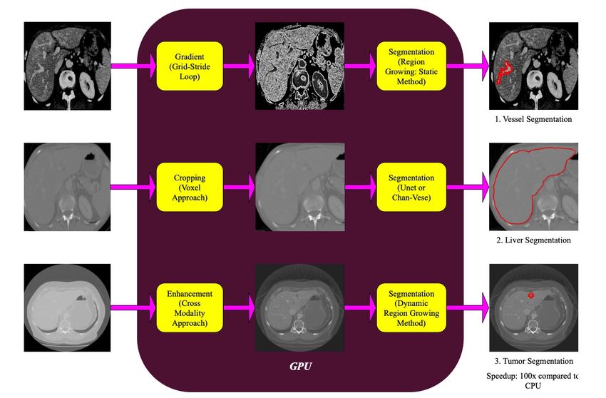
56Segmentation in Medical Image Analysis (I)
n Segmentation is used to obtain the area of an organ, a
tumor, etc.
Satpute et al., “Fast Parallel Vessel Segmentation,” CMPB 2020
Satpute et al., “GPU Acceleration of Liver Enhancement for Tumor Segmentation,” CMPB 2020
57
Satpute et al., “Accelerating Chan-Vese Model with Cross-modality Guided Contrast Enhancement for Liver Segmentation,” CBM 2020Segmentation in Medical Image Analysis (II)
n Seeded region growing is an algorithm for segmentation
q Dynamic data extraction as the region grows
Satpute et al., “Fast Parallel Vessel Segmentation,” CMPB 2020
Satpute et al., “GPU Acceleration of Liver Enhancement for Tumor Segmentation,” CMPB 2020
58
Satpute et al., “Accelerating Chan-Vese Model with Cross-modality Guided Contrast Enhancement for Liver Segmentation,” CBM 2020Region Growing with Kernel Termination and Relaunch
Start
Set a Seed
Terminate
Kernel
SRG
Kernel
Can
Launch
Stop Region
No Grow? Yes Kernel
CPU GPU
Slide credit: Nitin Satpute 59Region Growing with Inter-Block Synchronization
SRG
Start
Kernel
Yes IBS
Can
Set a Launch
Region
Seed Kernel
Grow?
No IBS-Inter Block
Terminate Synchronization
Stop
Kernel
CPU GPU
Slide credit: Nitin Satpute 60Inter-Block Synchronization for Image Segmentation
Satpute et al., “Fast Parallel Vessel Segmentation,” CMPB 2020. https://doi.org/10.1016/j.cmpb.2020.105430
Satpute et al., “GPU Acceleration of Liver Enhancement for Tumor Segmentation,” CMPB 2020. https://doi.org/10.1016/j.cmpb.2019.105285
Satpute et al., “Accelerating Chan-Vese Model with Cross-modality Guided Contrast Enhancement for Liver Segmentation,” CBM 2020.
https://doi.org/10.1016/j.compbiomed.2020.103930
61Collaborative Implementation
BFS on CPU or GPU?
n   Motivation
    q   Small-sized frontiers underutilize GPU resources
        n NVIDIA Jetson TX1 (4 ARMv8 CPU cores + 2 GPU cores)

        n   New York City roads

                                         10.0                                                50000
                                                                       CPU (4 threads)
                                          9.0                                                45000
                                                                       GPU (4x256 threads)
             Average execu:on :me (ms)

                                                                                                     Average nodes per fron:er
                                          8.0                                                40000
                                                                       Fron:er size
                                          7.0                                                35000
                                          6.0                                                30000
                                          5.0                                                25000
                                          4.0                                                20000
                                          3.0                                                15000
                                          2.0                                                10000
                                          1.0                                                5000
                                          0.0                                                0

                                                                00

                                                                  0

                                                                  6
                                                                 0

                                                                 0

                                                                 0

                                                                 0

                                                                 0

                                                                 0

                                                                 0

                                                                 0
                                                    0

                                                               10

                                                               19
                                                               20

                                                               30

                                                               40

                                                               50

                                                               60

                                                               70

                                                               80

                                                               90
                                                  10

                                                              10

                                                             -1

                                                             -1
                                                            1-

                                                            1-

                                                            1-

                                                            1-

                                                            1-

                                                            1-

                                                            1-

                                                            1-
                                                1-

                                                           1-

                                                          01

                                                          01
                                                          10

                                                          20

                                                          30

                                                          40

                                                          50

                                                          60

                                                          70

                                                          80

                                                         90

                                                        10

                                                        11
                                                            Fron:ers

                                                                                                                                 63
BFS: Collaborative Implementation (I)
n Choose CPU or GPU depending on frontier
// Host code
while(frontier_size != 0){
if(frontier_size < LIMIT){
// Launch CPU threads
}
else{
// Launch GPU kernel
}
}
n CPU threads or GPU kernel keep running while the
condition is satisfied
64BFS: Collaborative Implementation (II)
n Experimental results
q NVIDIA Jetson TX1 (4 ARMv8 CPU cores + 2 GPU cores)
1.2 CPU
CPU||GPU
1.0 GPU
Normalized execu9on 9me
0.8
0.6
0.4
15%
0.2
0.0
NY BAY
Graph
65Recommended Readings
n Hwu and Kirk, “Programming Massively Parallel Processors,”
Third Edition, 2017
q Chapter 12 - Parallel patterns:
graph search
66P&S Heterogeneous Systems
Parallel Patterns: Graph Search
Dr. Juan Gómez Luna
Prof. Onur Mutlu
ETH Zürich
Spring 2022
24 May 2022You can also read