Original Article Modelling chemical releases from fish farms: impact zones, dissolution time, and exposure probability
←
→
Page content transcription
If your browser does not render page correctly, please read the page content below
ICES Journal of Marine Science (2021), https://doi.org/10.1093/icesjms/fsab224
Downloaded from https://academic.oup.com/icesjms/advance-article/doi/10.1093/icesjms/fsab224/6453070 by guest on 09 December 2021
Original Article
Modelling chemical releases from fish farms: impact zones,
dissolution time, and exposure probability
*
Pål Næverlid Sævik , Ann-Lisbeth Agnalt , Ole Bent Samuelsen, and Mari Myksvoll
Institute of Marine Research, P.B. 1870 Nordnes, 5817 Bergen, Norway
∗
Corresponding author: tel:+47 55 23 85 00; e-mail: paal.naeverlid.saevik@hi.no
Sævik, P. N., Agnalt, A.L., Samuelsen, O. B., and Myksvoll, M. Modelling chemical releases from fish farms: impact zones, dissolution time, and
exposure probability. – ICES Journal of Marine Science, : –.
Received April ; revised October ; accepted October .
Tarpaulin bath treatments are used in open net-pen finfish aquaculture to combat parasitic infections, in particular sea lice. After treatment, the
toxic wastewater is released directly into the ocean, potentially harming non-target species in the vicinity. We model the dispersion of wastewater
chemicals using a high-resolution numerical ocean model. The results are used to estimate the impact area, impact range, dissolution time,
and exposure probability for chemicals of arbitrary toxicity. The study area is a fish-farming intensive region on the Norwegian western coast.
Simulations are performed at different release dates, each on locations. In our base case where the chemical is toxic at % of the treatment
concentration, the release of a m3 wastewater plume traverses a median distance of . km before being completely dissolved. The median
impacted area is . km2 and the median dissolution time is . hours. These figures increase to . km, . km2 , and hours, respectively, if the
chemical is toxic at . % of the treatment concentration. Locations within fjords have slower dissolution rates and larger impact zones compared
to exposed locations off the coast, especially during summer.
Keywords: aquaculture, bath treatment, dispersion, numerical ocean model, particle tracking, ROMS, sea lice, wastewater.
trolled, the parasite may multiply in large numbers in aquaculture-
Introduction dense areas due to the abundant availability of hosts (Heuch
Cage-based marine aquaculture of salmonids is a growing form of and Mo, 2001; Bergh, 2007), causing significant economic losses
food production. The industry produced 2.79 million tons globally (Costello, 2009; Kragesteen et al., 2019). Additionally, elevated par-
in 2018, worth 19.7 billion USD (FAO, 2020). Of these, 1.4 million asite abundance has a negative influence on the wild population of
tons were produced in Norway and 0.9 million tons in Chile. The Brown trout (Salmo trutta) (Skaala et al., 2014), as well as young
production consists primarily of Atlantic Salmon (Salmo salar) and wild Atlantic salmon who migrate from their river of origin towards
to a lesser degree rainbow trout (Oncorhynchus mykiss). A major the ocean during spring season (Hvidsten et al., 2007; Johnsen et al.,
challenge faced by the industry is parasitic infections by various 2020). To protect wild salmonid populations, Norwegian fish farm-
species of sea lice. In Europe and eastern North America, the species ers are required by law to keep the number of adult female lice per
Lepeophtheirus salmonis has caused the most concern (Johnson et fish below 0.2 in the spring season, and below 0.5 during the rest of
al., 2004; Torrissen et al., 2013; Taranger et al., 2015; Forseth et the year (Lovdata, 2018).
al., 2017), while Caligus rogercresseyi infestations has plagued fish One conventional method for reducing sea lice levels in open
farmers on the pacific coast of South America (Hamilton-West et net pens is in-situ bath treatments using anti sea-lice pharmaceu-
al., 2012). ticals. In this procedure, a fish cage under treatment is enclosed
Sea lice are ectoparasitic copepods that feed on the skin, blood, by a tarpaulin, and the therapeutant is added. After treatment, the
and mucus of its host (Kabata, 1974; Wootten et al., 1982). If uncon- tarpaulin is removed, and the treatment water is transported away
C The Author(s) 2021. Published by Oxford University Press on behalf of International Council for the Exploration of the Sea. This is an
Open Access article distributed under the terms of the Creative Commons Attribution License
(https://creativecommons.org/licenses/by/4.0/), which permits unrestricted reuse, distribution, and reproduction in any medium,
provided the original work is properly cited.
P. N. Sævik et al.
by ocean currents. Commonly used bath treatment chemicals con-
tain either deltamethrin, azamethiphos, or hydrogen peroxide as
active ingredients. While the treatment procedures are designed to
kill sea lice on farmed fish, the released wastewater may potentially
reach sensitive non-target organisms in the vicinity before being di-
luted to environmentally benign concentrations.
To protect marine wildlife, it is important to know how far from
the release site one can expect to find toxic concentrations. There
Downloaded from https://academic.oup.com/icesjms/advance-article/doi/10.1093/icesjms/fsab224/6453070 by guest on 09 December 2021
has been attempts to answer this question using field studies (Ernst
et al., 2014; Andersen and Hagen, 2016; Fagereng, 2016). Unfortu-
nately, field studies are not particularly well suited for this purpose.
The first problem is the heterogeneity of the turbulent dilution pro-
cess, which makes measurements highly sensitive to sampling loca-
tion and depth. The second problem is that only a relatively small
number of locations can be sampled simultaneously, making it dif-
ficult to obtain a clear picture of the plume size. The third problem
is that field studies of the required scale are expensive, and one can
not afford many repetitions of the same experiment. Thus, it is diffi-
cult to know whether the estimated impact area is representative for
releases occurring at other times or locations. Visible dye as used by
Ernst et al. (2014) can alleviate some of these problems, but only if
the main part of the plume stays close to the surface.
In the current research, we use a numerical ocean model to sim- Figure 1. Map of commercial marine salmonid fish farm locations
ulate the release and subsequent dilution of wastewater from fish within the study area. Red labelled dots indicate the position of the
farm tarpaulin operations. This allows us to monitor multiple vir- farms used as release points in the simulations.
tual chemical releases in full three-dimensions over a long time
period and obtain a complete overview over the resulting impact
zones. The ocean model have previously been used in a multitude
of applications in Norwegian fjords, and has shown good agreement have been used frequently to combat the problem. Of the 9433
with observational data (Asplin et al., 2020; Dalsøren et al., 2020). registered bath treatments in Norway from 2012 to 2020, 1870 were
While scenario-specific simulations of bath treatments have executed at farms within our study area (www.barentswatch.no).
been performed previously (Refseth et al., 2016, 2019; Parsons At the beginning of the year 2021, the region contained 145 marine
et al., 2020), these studies are limited in scope, and not designed commercial fish farming sites. In the current research, we have
to infer general statements about the expected size of the impact simulated releases from a representative sample of 16 locations
zones for arbitrary types of chemicals and release volumes. In (Figure 1). These include both exposed and sheltered locations on
the current research, we develop a statistical model using data the outer islands, sites in the outer and inner parts of the fjords,
from the numerical simulations, to estimate the sensitivity of the and sounds/narrows where the current circulation patterns are
impact zones and plume dilution rates with respect to chemical strongly constrained by the topography.
toxicity, release concentration, location, and time of release. We
also quantify how fast the exposure probability declines with the
distance from the release site. Hydrodynamic model
The Regional Ocean Modelling System (ROMS) is used to simu-
late the fjord currents (Shchepetkin and McWilliams, 2005). The
model setup is a horizontally refined version of NorKyst800 (Albret-
Methods sen et al., 2011), covering the study area at a horizontal resolution of
Study area 160 m × 160 m and a vertical resolution of 35 terrain-following gen-
The chosen study area is the western coast of Norway between lat- eralized sigma coordinate levels. The original NorKyst800 model,
itudes 59.5 ◦ N and 60.5 ◦ N. The region has two major fjord sys- which covers the Norwegian coast at 800 m × 800 m resolution, is
tems, Hardangerfjorden and Bjørnafjorden, which are connected to used as boundary conditions for the refined subgrid. The model
coastal water through multiple fjord mouths and inlets. The topog- setup has been validated against a wide range of hydrodynamic
raphy of the area is complex, consisting of several islands, fjords, measurements, and has been demonstrated to simulate realistic cur-
narrows, and bays. Off the coast, currents are dominated by the rents both within fjords and along the coast (Asplin et al., 2020;
Norwegian coastal current, which originates in the Baltic Sea and Dalsøren et al., 2020).
flows northward along the Norwegian coastline. Circulation pat- Atmospheric fields are provided from AROME MetCoOp (Me-
terns within the fjords are driven by tides, wind, and freshwater teorological Co-operation on Operational Numerical Weather Pre-
runoff from the surrounding rivers. The mean tidal range is small diction) 2.5 km, the main forecasting system at the Norwegian Me-
(∼1 m). Strong currents occur episodically in the upper ∼10 m, teorological Institute (Müller et al., 2017). Daily river flow rates are
generated by periods of strong winds. A brackish layer generates included in the simulations and based on estimates from the Nor-
shallow (∼5 m) outflows in periods with strong stratification close wegian Water Resources and Energy Directorate (NVE) through
to the surface (Asplin et al., 2014; Johnsen et al., 2014). their updated data series from all catchment areas in Norway (https:
Due to intensive aquaculture activity, the region has long ex- //nve.no). These data series use measured water flows to estimate
perienced elevated levels of sea lice. Tarpaulin bath treatments the total runoff along the coastline within each catchment area.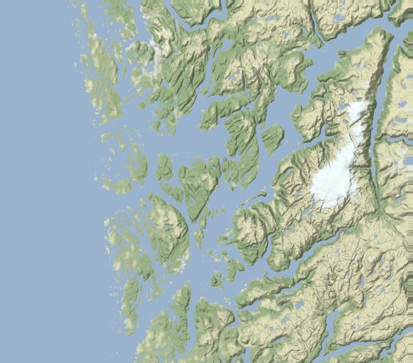
Modelling chemical releases from fish farms
Dispersion model Toxicity threshold
To model dispersion of chemicals, the Lagrangian Advection and Previously we have used the term “plume” in a loose sense. We now
Diffusion Model (Ladim) particle tracking software is used (https: define the wastewater plume more precisely as the portion of the
//github.com/bjornaa/ladim, version 1.1). Hourly ocean currents ocean where the normalized concentration of the bath treatment
from ROMS are used as forcing, with linear interpolation for inter- chemical exceeds a pre-defined toxicity threshold. In other words,
mediate time steps. A single release is represented by 100000 par- the plume boundary is a pre-defined concentration contour level.
ticles, initially contained within a volume of 40 m × 40 m × 10 m. The plume is considered dissolved if the normalized concentration
This is representative for the volume of a common large-class open is below the toxicity threshold everywhere. Furthermore, we define
Downloaded from https://academic.oup.com/icesjms/advance-article/doi/10.1093/icesjms/fsab224/6453070 by guest on 09 December 2021
net pen under a tarpaulin-based delousing operation, which may the impact zone as the region swept by the plume during its lifetime.
vary depending on the cage design and delousing technique (Vo- This includes any location which has experienced concentrations
lent et al., 2017). The particles are transported passively with the beyond the toxicity threshold at any point during the simulation,
flow, both horizontally and vertically. anywhere within the water column.
The main Ladim code base does not include vertical flow and There is not a single unique way to determine the toxicity thresh-
heterogeneous turbulence, which is important to model chemical old, as the harmful potential of a chemical varies among species and
dispersion rates correctly. These features were implemented as a may increase gradually with concentration. One strategy is to use
separate plugin module, available at https://github.com/pnsaevik/la the LC50 value (concentration that kills half of the organisms) of
dim_plugins (version 1.5.8). The plugin also includes modifications the most sensitive species in the vicinity, converted to normalized
to the current velocity interpolation scheme and the land collision concentration units. Values such as NOEC (no observed effect con-
treatment, to avoid artificial concentration buildup near shores. We centrations) or LC5 (concentration that kills 5 % of the organisms)
now briefly describe each of these improvements and refer to the can be used if a more conservative approach is desired.
source code for additional details. Table 1 lists LC50 values for some non-target species relevant to
As previously stated, we use velocity currents from ROMS, which Norwegian coastal waters, given an exposure time of 1 hour. Toxi-
are provided on a staggered Arakawa C-grid (Arakawa and Lamb, city data with respect to other species and endpoints can be found,
1977). In the main Ladim code base, velocities are bilinearly inter- for instance, in Refseth et al. (2016) and Urbina et al. (2019). In
polated, whereas the new plugin interpolates currents as in Döös the current work, we consider three explicit toxicity thresholds: 0.1,
et al. (2013) to keep the interpolated divergence consistent with 0.01, and 0.001. Estimates for intermediate toxicity thresholds can
the underlying numerical divergence. This eliminates one source of be obtained by interpolation.
artificial particle clustering. Furthermore, vertical velocity is com- When simulation results are compared with actual chemical re-
puted from the horizontal divergence and used to advect particles in leases, one should also take the release volume into account. Halv-
the vertical direction. In the horizontal direction, particles are ad- ing the release volume will have an effect similar to halving the re-
vected using a Runge–Kutta 4th order scheme, which reduces the lease concentration, except in the vicinity of the fish farm. This is
probability that a particle ends up on land. If a land collision should because the plume is initially small and will expand to twice its size
happen nevertheless, the particle is repositioned randomly within within a relatively short amount of time. One can account for vary-
the grid cell it originated from. ing release volumes by using the following definition of the toxicity
Heterogeneous turbulent mixing is modelled as a stochastic dif- threshold,
ferential equation (Gräwe, 2011), and solved numerically using the Toxicity Reference volume Harmful concentration
scheme of LaBolle et al. (2000). This scheme entirely avoids arti- = × (1)
threshold Release volume Release concentration
ficial particle clustering for heterogeneous mixing profiles. In the
horizontal direction, turbulent mixing is computed using the for- where “harmful concentration” could be LC50 or any other relevant
mulation of Smagorinsky (1963), in the form given by Kantha and endpoint, and “reference volume” is the release volume used in our
Clayson (2000), Equation (1.17.6). In the vertical direction, turbu- simulations (16000 m3 ).
lent mixing is taken directly from ROMS, which uses the Generic
Length Scale model to compute the mixing coefficient (Umlauf
and Burchard, 2003). For numerical stability reasons, vertical mix- Outcome parameters
ing is sampled at 5 m intervals and capped at a maximal value of For each simulated chemical release, we computed four different
0.01 m2 /s. outcome parameters related to plume exposure. Here we define
The dispersed particle field was converted to a continuous con- each outcome parameter in order and briefly discuss their ecologi-
centration field using a standard box counting approach, where the cal significance.
domain of interest was divided into blocks of 100 m × 100 m in the The impact area is simply the area of the impact zone. Impact
horizontal plane and 1 m in the vertical direction. The particle con- area is relevant, for instance, if the sensitive species under consider-
centration was computed by dividing the number of particles by ation is plentiful and can reproduce relatively quickly. If the typical
the volume of the block. The normalized concentration is the par- impact area is small compared to the species’ habitat, occasional
ticle concentration divided by the initial particle concentration in- plume exposures may be of little concern.
side the fish cage (6.25 particles per m3 ). The actual chemical con- The impact range is the horizontal distance from the release point
centration is the normalized concentration times the initial release to the farthest edge of the plume during its lifetime. A sensitive
concentration. species can be considered relatively safe from exposure if the typi-
We performed 61 releases for each of the 16 locations, one every cal impact range is shorter than the distance between its habitat and
sixth day from January 4, 2020 to December 29, 2020, all starting the release point.
at 12:00. The particles were tracked for 48 hours. This allowed the The dissolution time is the time elapsed from the tarpaulin is re-
plume to be completely dissolved within the simulation period, with leased until the plume is completely dissolved, i.e. the normalized
a few exceptions. concentration has fallen below the toxicity threshold everywhere.
P. N. Sævik et al.
Table 1. LC values for a selected number of species with respect to hydrogen peroxide (H2 O2 ), deltamethrin (Deltam.), and azamethiphos
(Azam.).
Species (life stage) Chemical LC50 (g / L) LC50 (normalized) Source
−2 −2
Calanus spp. (CV) H O 7.7 × 10 5.1 × 10 (Escobar-Lux et al., )
Calanus spp. (adult) H O 3.1 × 10⁻² 2.1 × 10⁻² (Escobar-Lux et al., )
Homarus gammarus (stg.I) Deltam. 2.6 × 10⁻⁹ 1.3 × 10⁻³ (Parsons et al., )
Homarus gammarus (stg.I) Azam. 4.3 × 10⁻⁵ 4.3 × 10⁻¹ (Parsons et al., )
Downloaded from https://academic.oup.com/icesjms/advance-article/doi/10.1093/icesjms/fsab224/6453070 by guest on 09 December 2021
Homarus gammarus (stg.II) Deltam. 2.9 × 10⁻⁹ 1.5 × 10⁻³ (Parsons et al., )
Homarus gammarus (stg.II) Azam. 2.1 × 10⁻⁵ 2.1 × 10⁻¹ (Parsons et al., )
Saccharina latissima (juvenile) H O 8.1 × 10⁻² 5.4 × 10⁻² (Haugland et al., )
Meganyctiphanes norvegicus H O 4.9 × 10⁻³ 3.3 × 10⁻³ (Escobar-Lux and Samuelsen, )
Palaemon elegans Deltam. 1.2 × 10⁻⁷ 6.0 × 10⁻² (Brokke, )
Praunus flexuosus Deltam. 1.1 × 10⁻⁷ 5.5 × 10⁻² (Brokke, )
Ophryotrocha spp. H O 6.4 × 10⁻² 4.3 × 10⁻² (Fang et al., )
Exposure time is hour plus a recovery period. Normalized concentrations are relative to standard treatment concentrations (Jansen, ),
which is . g/L for hydrogen peroxide, μg/L for deltamethrin, and μg/L for azamethiphos.
This is an upper limit to exposure time, while most organism– Covariates for exposure probability (EP, continuous between 0
plume encounters will be of significantly shorter duration. Non- and 1) are the same as in Equation (2), with an additional covariate:
target species that are robust to short chemical exposures are also distance from release location (D, continuous, in km). Interaction
relatively unharmed by chemical releases with a short dissolution terms between D and the other covariates are included. A logistic
time. model was used for the outcome parameter, with model equation
The exposure probability is the probability of being exposed to
the wastewater plume at distance D from the release point. To com- logit EP = α + βCC + βU U + βT s (T ) + βL L
pute exposure probability, we first created a set of concentric, donut-
shaped regions around the release point, each having a width of + D × (βD + βDCC + βDU U + βDT s (T ) + βDL L)
1 km. Within each region, the exposure probability was defined as (3)
the impact area divided by the total ocean area.
The model is fitted using sea cells only, i.e. we estimate the prob-
ability of a sea cell at a certain distance being hit by the plume. Each
Statistical regression model cell is treated as an independent observation, which is not strictly
We performed a series of regression analyses to estimate the effect true for cells in close proximity. Consequently, the confidence in-
of input variables on the four outcome parameters defined above. tervals produced by the regression are too narrow, and we do not
We used the same type of model equation for impact area, impact report them in the paper. The estimated regression coefficients are
range, and dissolution time, while exposure probability is modelled still unbiased since the dataset is produced by a balanced design.
by a second type of equation. Model assumptions (normality, ho- To use Equations (2) and (3) for predictions, coefficients re-
moscedasticity, etc.) were verified by plotting residuals vs. fitted val- lated to location and time can be set to zero if an average value
ues and vs. each covariate, and by quantile-quantile plots. Statistical is desired. For toxicity thresholds other than the reference thresh-
significance of each covariate was assessed by dropping individual olds, interpolation on a log scale is recommended. If the toxicity
variables and comparing Akaike Information Criterion (AIC) val- threshold C is between 0.1 and 0.01, one could set βC[0.001] = 0 and
ues. We also computed the change in Pearson correlation coefficient βC[0.1] = 2 + log10C, where the superscript of βC indicate the factor
(R2 ) and root mean squared error for each covariate exclusion, as a level. If the toxicity threshold is between 0.01 and 0.001, we have
measure of their explanatory power. βC[0.1] = 0 and βC[0.001] = −2 − log10C.
Covariates for impact area (IA, continuous, in m), impact range All statistical analyses were conducted in R Studio Elderflower
(IR, continuous, in m), and dissolution time (DT, continuous, in s) (RStudio Team, 2019). Figures were either produced in Python 3 us-
are the toxicity threshold (C, categorical with levels 0.1, 0.01 [refer- ing matplotlib version 3.2.2 (Hunter, 2007) and holoviews version
ence] and 0.001), the ocean current speed at 5 m depth (U, contin- 1.13.3 (Rudiger et al., 2020), or in R Studio using ggplot2 version
uous, in m/s), time of the year (T, in Julian days), and location (L, 3.3.2 (Wickham, 2016) and ggmap version 3.0.0 (Kahle and Wick-
categorical with 16 levels, deviance contrast coding). The outcome ham, 2013).
parameters were log10 transformed, both to normalize the data and
because data exploration indicated a multiplicative dependence on
the covariates. The only transformed covariate is T, which is spline Results
smoothed. The model equation is
Model validation
log10 μ = α + βCC + βU U + βT s (T ) + βL L (2) Quantile-quantile plots and residual distribution plots generated
from the linear regression model indicated no problems except for
where μ represents the expectation value of any of the outcome pa- a somewhat fat-tailed residual distribution outside of 2 SD. In other
rameters, s is a 4-knot cyclic spline smoother, α is the intercept, and words, the regression model may underpredict the occurrence of
{β i } are the regression coefficients, some of which are multi-valued rare outcomes. Analysis of AIC values showed that all covariates
(i.e. those belonging to categorical or spline-smoothed covariates). and interaction terms were significant. The R2 correlation coeffi-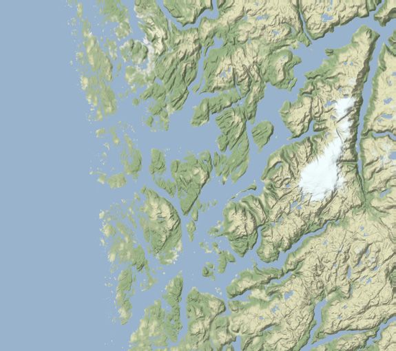
Modelling chemical releases from fish farms
Table 2. Root mean squared error for the models defined by Equa- by 0.1 m/s (Table 4). Compared with the reference toxicity thresh-
tion () including all covariates (bottom row), compared with models old of 0.01, the mean impact range increases by a factor of 3.1 if the
where a single covariate is removed. threshold is 0.001 and reduces by a factor of 8.5 if the threshold is
0.1. The magnitudes of location and release time effects (standard
Covariate Impact Impact Dissolution
deviation across possible values) correspond to a change in dissolu-
removed area range time
tion time by 35 % and 20 %, respectively. The residual standard de-
C . . . viation is 0.20, which corresponds to a change of dissolution time
L . . . by 58 % (Table 2).
Downloaded from https://academic.oup.com/icesjms/advance-article/doi/10.1093/icesjms/fsab224/6453070 by guest on 09 December 2021
T . . .
U . . .
(None) . . .
Exposure probability
Covariates are C (toxicity threshold), L (location), T (release time), and Estimated coefficients for the exposure probability model given
U (ocean current speed at m depth). by Equation (3) are shown in Table 5. The exposure probability de-
clines exponentially with distance, with a decline rate highly depen-
dent on the toxicity threshold (Figure 6). For C = 0.1, the exposure
cients of the regression models were 0.94 for impact area, 0.86 for probability is estimated by the model to be 10 % at 0.1 km, 1 % at
impact range, and 0.91 for dissolution time. 0.6 km, and 0.1 % at 1.1 km. For C = 0.01, the probability is esti-
mated to 10 % at 1.1 km, 1 % at 2.7 km, and 0.1 % at 4.2 km. For C =
0.001, the probability is estimated to 10 % at 3.4 km, 1 % at 6.8 km,
Impact area, impact range, and dissolution time and 0.1 % at 10.0 km. Figure 7 shows an overlay of impact zones for
The impact area, impact range, and dissolution time are all very all simulated release times and locations, which gives a visual im-
sensitive to the toxicity threshold, which explains most of the vari- pression of the exposure probability and its spatial variation.
ation in the dataset (Table 2). The remaining covariates show sig- It may be surprising that the exposure probability is small at dis-
nificant effects as well, but they do only slightly improve the predic- tances comparable to the median impact range. The reason is that
tive power of the regression. In other words, there is a large residual exposure probability represents a randomly chosen direction from
variation caused by shifting current patterns in the region around the farm. In contrast, the impact range is the distance from the farm
the farm, which are not predictable from simple statistics. As an ex- to the farthest edge of the impact zone, which is not a randomly
ample of the variation seen in the simulation data, Figure 2 features chosen direction.
three simulated releases from the same farm within the same time The effects of location and time of year on exposure probabil-
of year, with widely different impact ranges. ity are statistically significant, but of smaller magnitude compared
The median impact area was 0.04 km2 , 0.90 km2 , and 6.99 km2 with the toxicity threshold (Figure 8). For instance, the exposure
for toxicity thresholds of 0.1, 0.01, and 0.001, respectively (Table 3). probability for C = 0.01 at 2 km distance from Farm C (highly ex-
Compared with the reference toxicity threshold of 0.01, the mean posed location) equals the exposure probability 3.1 km from Farm
impact area increases by a factor of 8.0 if the threshold is 0.001 and P (highly sheltered location). Time of year is somewhat less impor-
reduces by a factor of 21.4 if the threshold is 0.1 (Table 4). Impact tant: Wintertime exposure probability for C = 0.01 at 2 km distance
area increases by only 1 % if the local current speed at 5 m depth equals the summertime exposure probability at 2.4 km distance.
increases by 0.1 m/s. The magnitudes of location and release time Note that exposure probability as defined in this paper only in-
effects (standard deviation across possible values) correspond to an cludes the horizontal direction. To complement this, we also com-
impact area change of 48% and 19%, respectively. Figure 3 illustrates puted the maximal depth penetration of the simulated wastewater
the effect of location for each release site, while Figure 4 plots the plumes for different toxicity thresholds (Figure 9). When C = 0.1,
effect of time. Note that the trends shown in Figure 4 may be specific 90 % of the simulated wastewater plumes stay within the upper 10 m
to the year 2020, as interannual variation was not a part of this study. for the entire simulation. For C = 0.01 and C = 0.001, 90 % of the
The residual standard deviation is 0.24, which corresponds to an simulated wastewater plumes stay within the upper 13 m and 18 m,
impact area change of 73 % (Table 2). respectively. The plumes are more quickly dissolved in the upper
The median impact range was 0.25 km, 1.90 km, and 5.87 km for 5 m, due to stronger turbulent mixing rates near the surface.
toxicity thresholds of 0.1, 0.01, and 0.001, respectively (Table 3).
Compared with the reference toxicity threshold of 0.01, the mean
impact range increases by a factor of 3.1 if the threshold is 0.001
and reduces by a factor of 7.6 if the threshold is 0.1 (Table 4). Im- Discussion
pact range increases by 14% if the local current speed at 5 m depth Relative importance of covariates
increases by 0.1 m/s. The magnitudes of location and release time Toxicity threshold is the most influential covariate, and the only
effects (standard deviation across possible values) correspond to a covariate that dominates over residual variation. The strong depen-
change of impact range by 35 % and 9 %, respectively. The resid- dence on toxicity threshold is expected, as we investigated a wide
ual standard deviation is 0.23, which corresponds to 71 % change range of values spanning three orders of magnitude. The entire
of impact range (Table 2). range is relevant since both the low and high end of the range are
The median dissolution time was 0.83 hr, 6.83 hr, and 21.0 hr for encountered in management applications. Even though the strong
toxicity thresholds of 0.1, 0.01, and 0.001, respectively (Table 3). The effect of toxicity threshold may seem obvious, regulations do not
plume growth phase was revealed to be about half as long as the necessarily take this effect into account. For instance, Norwegian
shrinkage phase, but there are large individual differences (Figure authorities do not allow tarpaulin bath treatments within 500 m of
5). The linear regression model predicts an increase in mean disso- officially recognized shrimp fields and cod spawning grounds, re-
lution time by 33 % if the local current speed at 5 m depth decreases gardless of the release volume, concentration, or type of chemical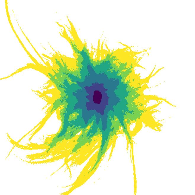
P. N. Sævik et al.
Downloaded from https://academic.oup.com/icesjms/advance-article/doi/10.1093/icesjms/fsab224/6453070 by guest on 09 December 2021
Figure 2. Simulation results for Farm D at three different release times in June and July, demonstrating large variation in impact range. Note the
different spatial scales from left to right. Colours indicate the largest recorded concentration within the water column over the course of the
simulation. Black circles represent the impact range for a toxicity threshold of ..
Table 3. Median values for impact area, impact range, and dissolution time, grouped by the toxicity threshold value.
Toxicity threshold Impact area (km) Impact range (km) Dissolution time (hr)
. . [., .] . [., .] . [., .]
. . [., .] . [., .] . [., .]
. . [., .] . [., .] . [., .]
Values in square brackets are the first and third quartiles.
Table 4. Regression coefficients for the models defined by Equation The mean impact area, dissolution time, and impact range are
(), with covariates U (ocean current speed at m depth, in m/s), C all peaking during the summer season. This is expected as strati-
(toxicity threshold, relative to release concentration), L (location, fication is stronger in the summer, especially in the fjords, due to
levels), and T (time, -knot cyclic spline). increased freshwater runoff and elevated surface temperatures. The
overall effect is not as large as the location effect, but there might be
Covariate log10 IA log10 IR log10 DT
specific locations where the seasonal effect is more pronounced.
(Intercept) . (.) . (.) . (.) Location and local current speed are correlated but give inde-
U . (.) . (.) − . (.) pendent contributions to the outcome parameters. While strong
C[.] . (.) . (.) . (.) currents may transport the plume faster, it often leads to increased
C[.] − . (.) − . (.) − . (.) turbulent mixing and rapid dissolution. It seems like these effects
L (magnitude) . . . cancel out when it comes to impact area, leaving only a weak corre-
T (magnitude) . . . lation. The effect of current speed on impact range and dissolution
Standard errors are shown in parentheses. For location and release time is stronger, but not as important as location.
time, only the typical magnitude (standard deviation across possible
values) is shown. Outcome parameters are IA (impact area, in m2 ), IR
(impact range, in m), and DT (dissolution time, in s). Implications for policymakers
Our results demonstrate that chemicals released from tarpaulin
bath treatments can affect large areas far from the release point.
Factors that strongly influence the damage potential are the release
used (Lovdata, 2019). A buffer zone of 500 m offers a good level of volume and the harmful concentration relative to the release con-
protection from releases having a toxicity threshold of 10% but is centration. Policymakers may want to consider restrictions on bath
less effective when the toxicity threshold is 1% or smaller. treatment activity that occur close to sensitive habitats, especially
Chemical releases in sheltered areas within fjords appear to have if the active chemical is harmful at small concentrations. Restric-
wider impact ranges, larger impact zones, and longer dissolution tions may include banning the use of certain chemicals, capping
times compared to more exposed areas off the coast. Ocean masses the permissible release volume or restricting the number of allowed
within fjords are often strongly stratified, which inhibits vertical tarpaulin operations per year. Bath treatments may alternatively be
mixing and leads to slower dissolution rates. In addition, freshwa- performed using wellboats where the wastewater is released gradu-
ter runoff from rivers can create a persistent fjord outflow in the ally while the boat is moving, contributing to rapid dilution of the
upper layers, which may transport the plume further away with- chemicals (Refseth et al., 2019). With wellboats, the treatment wa-
out dissolving it. The mean effect of location is moderate compared ter can also be transported away from sensitive habitats before being
to the importance of the toxicity threshold. Still, the difference be- released.
tween the most sheltered and most exposed location in our dataset Even if the release volume and type of chemical is fixed, the im-
is comparable to the difference between C = 0.001 and C = 0.01. pact range varies considerably. This is primarily due to variations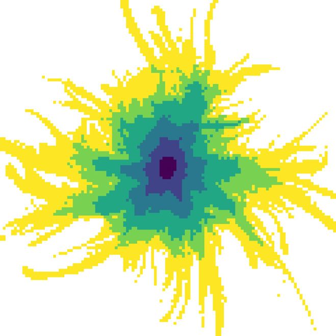
Modelling chemical releases from fish farms
Downloaded from https://academic.oup.com/icesjms/advance-article/doi/10.1093/icesjms/fsab224/6453070 by guest on 09 December 2021
Figure 3. Effect of location on impact area (IA), impact range (IR), and dissolution time (DT) according to the model defined by Equation ().
2.68 ± 0.24 (mean ± SD), i.e. an interval of 275 m–831 m. This in-
terval represents the most probable impact range, but shorter and
longer impact ranges are also possible.
If the location is known to be a sheltered fjord location, we can set
βL = 0.13 (1 SD, Table 4), which raises the predicted impact range
by 35%. Conversely, if the location is known to be highly exposed,
we can set βL = −0.13, which reduces the impact range to 74% of
the original.
Next, assume that we are interested in a specific kelp forest lo-
cated 900 m from the release point. The probability that the plume
will reach this location is 1.0 % according to our statistical model. If
there are 100 kelp forests at 900 m distance from the farm, it is ex-
Figure 4. Effect of release time on impact area (IA), impact range pected that one of these are exposed to harmful concentrations after
(IR), and dissolution time (DT) according to the model defined the release. Note that this probability does not take vertical distri-
by Equation (). Shaded bands denote % confidence intervals. bution into account. The plume is most likely to stay in the upper
10–20 m of the water column. Some of the kelp may be growing at
depths of 20–30 m, and the probability of exposure to these areas is
in the current patterns in the wider region around the release point. smaller.
On average, some locations give larger impact ranges than others, The log10 impact area is estimated to 5.04 ± 0.23 (mean ± SD),
but the variation within each location is usually greater than the dif- which equals an interval of 0.06 km2 –0.19 km2 . This is an upper
ference between them. The large amount of variation makes it dif- limit to the amount of kelp that can be exposed to harmful concen-
ficult to define an absolute “safety distance” from the release point, trations by a single release, which is only attained if the plume is
beyond which no harmful effects can be expected. Instead, there is released in the middle of a kelp forest.
a wide region around the farm where harmful exposure is unlikely, The predicted dissolution time is 1.0 hr–2.4 hr (mean ± SD).
but not impossible. Policy makers will have to decide whether this It is recommended that no additional releases are performed
risk is acceptable or not. within this time period. Otherwise, the concentration of the new
release is added to the remaining concentration of the old re-
lease, which slows down dilution and increases the impact area
Sample application: kelp forests and range. Plume dissolution time is not directly related to
Below, we apply our statistical results to assess the harmful po- the exposure time for individual kelp plants, which is poten-
tential of a hydrogen peroxide release on nearby populations of tially much shorter than the time it takes to dissolve the plume
sugar kelp (Saccharina latissima). We consider a tarpaulin opera- completely.
tion where 18000 m3 of treatment water is released, with a treatment All numbers presented above are based on the LC50 value. An-
concentration of 1500 mg/L and a local current speed at 5 m depth other relevant endpoint is the EC50 value of 28 mg/L (Haugland et
of U = 0.1 m/s. al., 2019), which includes sub-lethal effects of reduced photosyn-
The LC50 of juvenile sugar kelp at 1 hour exposure to H2 O2 was thetic capacity and efficiency. Assuming unchanged treatment vol-
estimated by Haugland et al. (2019) to be 81 mg/L, which is 0.054 ume of 18000 m3 and treatment concentration of 1500 mg/L, the
times the release concentration. Scaling by the release volume, this toxicity threshold drops from 0.048 to 0.014 by using this endpoint.
equals a toxicity threshold of C = 0.048, which is halfway between This increases the mean impact range from 480 m to 1200 m, and
our reference thresholds of 0.1 and 0.01. Interpolating on a log the mean impact area from 0.11 km2 to 0.45 km2 . Similarly, the im-
scale as described in the methods section, we get βC[0.1] = 0.68 and pact range and area increase if the treatment concentration or treat-
βC[0.001] = 0. From Equation (2), we predict a log10 impact range of ment volume is increased.
P. N. Sævik et al.
Downloaded from https://academic.oup.com/icesjms/advance-article/doi/10.1093/icesjms/fsab224/6453070 by guest on 09 December 2021
Figure 5. Instantaneous area of the plume at different points in time for all simulations, grouped by toxicity threshold (C). Note the different
spatial and temporal scales.
Table 5. Coefficients for the regression model in Equation (), which threshold of 0.01 in our simulations thus corresponds to a field con-
estimates exposure probability (EP). centration of 26.25 mg/L in their simulations. Visual inspection of
the provided figures suggests that the impact range of their simu-
Covariate logit EP lations are similar to ours, but a direct comparison is difficult since
(Intercept) − . they only report the largest observed concentration over a course of
C [.] . 48 individual release times. The report states that concentrations of
C [.] − . 10 mg/L can occur ∼5 km from the release, which fits well with our
U − . own data.
L (magnitude) . Ernst et al. (2014) performed field measurements of azame-
T (magnitude) . thiphos and deltamethrin after six separate operational tarpaulin
D − . bath treatments in New Brunswick, Canada. Fluorescent dye was
D × C[.] . added to track the wastewater plume. The treatment volume was
D × C[.] − .
800 m3 , which is 0.05 times the reference volume of 16000 m3 used
D×U .
D × L (magnitude) .
in our simulations. A toxicity threshold of 0.1 in our dataset there-
D × T (magnitude) . fore corresponds to a dilution of 1:200 in their field study. The
plumes tracked in their study reached this dilution level within
Covariates in the table are D (distance from release location, in km), 150 m to 1700 m from the release site. Our data suggest an impact
U (ocean current speed at m depth, in m/s), C (toxicity threshold), L range of 160 m–430 m at this toxicity threshold (25%–75 % per-
(location, levels), and T (time, -knot cyclic spline). For location and centile), with a maximal value of 2 km. Thus their measurements
release time, only the typical magnitude (standard deviation across agree with our simulations. One should also take into account that
possible values) is shown. their field samples are point measurements taken in the middle of
the plume, while our model data represent the average concentra-
tion within computational cells of 100 m × 100 m. It is therefore
not surprising that their measurements are somewhat at the high
end of the scale compared with the simulations.
Model limitations
The main limitation to the simulation model is that released chem-
icals are assumed to follow the currents passively. This may give
misleading results for hydrogen peroxide if the water column is
well-mixed, since the plume may sink downwards due to its density
(Refseth et al., 2019). Also, in a strongly stratified water column,
the well-mixed treatment water may migrate into a narrow vertical
Figure 6. Probability of being exposed to harmful concentration at a layer upon tarpaulin release. Neither of these effects are included
certain distance from the release point. Markers represent the mean in the particle tracking model, and future research is required to
probability from simulations, across all farms and release times. quantify them. Another effect not included in the model is addi-
Vertical lines represent the % confidence interval of the mean. tional dispersion and drift due to surface waves. We do not expect
Sloped lines represent the regression mean as defined by Equation this to be a significant source of error, but large wave activity may
().
improve the plume dilution rate somewhat. Tarpaulin operations
are mostly performed when the wave height is small, due to techni-
Comparison with previous works cal considerations.
Refseth et al. (2019) performed simulations of hydrogen peroxide Our model does not currently include the vertical and hori-
releases from four Norwegian fish farm locations, using a treatment zontal migration behaviour of non-target species. Impact assess-
volume of 21000 m3 and a treatment dose of 2000 mg/L. A toxicity ments must take this behaviour into account as well. For instance,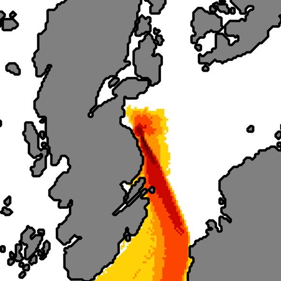
Modelling chemical releases from fish farms
Downloaded from https://academic.oup.com/icesjms/advance-article/doi/10.1093/icesjms/fsab224/6453070 by guest on 09 December 2021
Figure 7. Overlay of exposure areas for all release times and locations, grouped by toxicity threshold (C). Note the different length scale in each
subfigure. Colours indicate the fraction of releases exceeding the toxicity threshold.
al., 2003). The reported half-life varies wildly in the literature, most
are in the order of days or weeks while some are in the order of hours
[see Lyons et al. (2014) and the references therein]. The half-life of
deltamethrin is estimated to 18 hours in the aqueous phase (Erst-
feld, 1999), but the chemical is also strongly lipophilic and attaches
to particles, sediment, and organisms (Ernst et al., 2014), thus re-
moving it from the water phase. Azamethiphos is water soluble and
more stable, with a half-life in the order of ∼10 days (Worthing and
Walker, 1987). In general, any degradation process that happen on
time scales comparable to the dissolution time will reduce the im-
pact range, area, and dissolution time. For most applications, dis-
persion by hydrodynamic currents is still expected to be the domi-
nant effect.
In our simulations, we assume that the ocean is pristine at the
time of the release. In practice, cages are often treated successively,
with pulses of chemicals released repeatedly into the ocean. Multi-
Figure 8. Impact of location times distance on exposure probability, ple exposures have the potential of being harmful to sensitive organ-
as estimated by the regression model in Equation (). The magnitude isms even if the chemical is highly diluted (Bechmann et al., 2019).
must be interpreted using the logit link of the regression model.
deep-dwelling species are less likely to encounter neutrally buoy- Conclusions and further work
ant plumes, which will mostly stay in the upper layers of the water We have performed high-resolution simulations of chemical re-
column. Zooplankton often have a diurnal vertical migration cy- leases from fish farms and summarized the results in a statistical re-
cle, which gives a higher probability of exposure during night-time gression model. Four parameters quantifying the damage potential
(Stich and Lampert, 1981; Lampert, 1989; Heywood, 1996). Hori- were estimated: the impact area, impact range, dissolution time, and
zontal migration behaviour may influence both the exposure prob- exposure probability. The main variable controlling all of these pa-
ability and the exposure time. Organisms who follow the ocean cur- rameters is the toxicity threshold, which is the amount of large-scale
rents passively stay in the same body of water for a long time and are dilution required to neutralize the released chemical, scaled by the
less likely to encounter a nearby plume than stationary or upstream- release volume [Equation (1)]. If the released volume is large and the
swimming species. On the other hand, if a passively transported or- wastewater is highly toxic, harmful concentrations are found over
ganism does get mixed into the plume, it is likely to stay in the plume 20 km from the release point in rare instances. At exposed loca-
for a longer time. One should also note that few organisms are truly tions, plumes dissolve faster, and the average impact area and range
passive drifters in the vertical direction. For instance, buoyant and are smaller. Still, the difference between locations were smaller than
upwards-swimming plankton may be temporarily captured by lo- the variation within locations. Seasonal differences were statistically
cal convergence zones (Skarðhamar et al., 2007; Mann and Lazier, significant, but smaller than the effect of location.
2013). This increases the chance of exposure to nearby plumes pass- Further research may be directed at quantifying the exposure
ing through the convergence zone. probability of specific species by coupling the plume drift model to a
Degradation of the released substances is not included in the biological model of chemical sensitivity and vertical/horizontal mi-
model. The mechanisms behind degradation are manifold, depend- gration, possibly including chemical degradation. Further research
ing on the chemical in question. For instance, hydrogen peroxide is may also be directed at estimating impact zones for well boat re-
an oxidising agent, which may react with organic substances in the leases. An additional topic for further study is the effect of ocean
seawater, catalysed by light and various planktonic species (Wong et stratification and wastewater density on the initial plume distribu-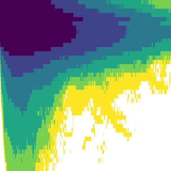
P. N. Sævik et al.
Downloaded from https://academic.oup.com/icesjms/advance-article/doi/10.1093/icesjms/fsab224/6453070 by guest on 09 December 2021
Figure 9. Overlay of plume vertical distributions as a function of time, for all release times and locations, grouped by the toxicity threshold (C).
Colours indicate the fraction of simulated wastewater plumes reaching the indicated depth.
tion, which is not studied in this paper. One may also consider a fjord, Norway. Estuarine, Coastal and Shelf Science, 246: 107028.
broader geographical range of release sites. Simulations from mul- https://doi.org/10.1016/j.ecss.2020.107028.
tiple years could be useful to study interannual variations. Döös, K., Kjellsson, J., and Jönsson, B. 2013. TRACMASS—a La-
grangian trajectory model. In Preventive Methods for Coastal Pro-
tection: Towards the Use of Ocean Dynamics for Pollution Control,
pp. 225–249. Ed. by Soomere, Tand and Quak, T. Springer Inter-
Data availability national Publishing, Heidelberg. https://doi.org/10.1007/978-3-31
The model data underlying this article will be shared on reasonable 9-00440-2_7.
Ernst, W., Doe, K., Cook, A., Burridge, L., Lalonde, B., Jackman, P.,
request to the corresponding author. Aubé, J. G. et al. 2014. Dispersion and toxicity to non-target crus-
taceans of azamethiphos and deltamethrin after sea lice treatments
References on farmed salmon, Salmo salar. Aquaculture, 424-425: 104–112.
Albretsen, J., Sperrevik, A. K., Staalstrøm, A., Sandvik, A. D., Vikebø, https://doi.org/10.1016/j.aquaculture.2013.12.017.
F., and Asplin, L. 2011. NorKyst-800 Report No. 1: User Manual and Erstfeld, K. M. 1999. Environmental fate of synthetic pyrethroids dur-
Technical Descriptions. 2–2011. Fisken Og Havet.. Institute of Ma- ing spray drift and field runoff treatments in aquatic microcosms.
rine Research. Chemosphere, 39: 1737–1769. https://doi.org/10.1016/S0045-6535
Andersen, P. A., and Hagen, L. 2016. Fortynningsstudier: Hydrogenper- (99)00064-8.
oksid. 156-8–16. Aqua Kompetanse AS. Escobar-Lux, R. H., Fields, D. M., Browman, H. I., Shema, S. D., Bjel-
Arakawa, A., and Lamb, V. R. 1977. Computational design of the ba- land, R. M., Agnalt, A-L., Skiftesvik, A. et al. 2019. The effects of
sic dynamical processes of the UCLA general circulation model. In hydrogen peroxide on mortality, escape response and oxygen con-
Methods in Computational Physics: Advances in Research and Ap- sumption of Calanus spp. FACETS, 4, 626–637. https://doi.org/10.1
plications, pp. 174–267. Academic Press, New York. 139/facets-2019-0011.
Asplin, L., Albretsen, J., Johnsen, I.A., and Sandvik, A. D. 2020. The hy- Escobar-Lux, R. H., and Samuelsen, O. B. 2020. The acute and delayed
drodynamic foundation for salmon lice dispersion modeling along mortality of the Northern krill (Meganyctiphanes norvegica) when
the Norwegian coast. Ocean Dynamics, 70: 1151–1167. https://doi. exposed to hydrogen peroxide. Bulletin of Environmental Contam-
org/10.1007/s10236-020-01378-0. ination and Toxicology, 105: 705–710. https://doi.org/10.1007/s001
Asplin, L., Johnsen, I. A., Sandvik, A. D., Albretsen, J., Sundfjord, V., 28-020-02996-6.
Aure, J., and Boxaspen, K. K. 2014. Dispersion of salmon lice in the Fagereng, M. B. 2016. Bruk av hydrogenperoksid i oppdrettsanlegg;
Hardangerfjord. Marine Biology Research, 10: 216–225. https://do fortynningstudier og effekter på blomsterreke (Pandalus montagui).
i.org/10.1080/17451000.2013.810755. Master thesis. https://bora.uib.no/handle/1956/13008.
Bechmann, R. K., Arnberg, M., Gomiero, A., Westerlund, S., Lyng, E., Fang, J., Samuelsen, O. B., Strand, Ø., and Jansen, H. 2018. Acute toxic
Berry, M., Agustsson, T. et al. 2019. Gill damage and delayed mor- effects of hydrogen peroxide, used for salmon lice treatment, on the
tality of northern shrimp (Pandalus borealis) after short time ex- survival of polychaetes Capitella sp. and Ophryotrocha spp. Aqua-
posure to anti-parasitic veterinary medicine containing hydrogen culture Environment Interactions, 10: 363–368. https://doi.org/10
peroxide. Ecotoxicology and Environmental Safety, 180: 473–482. .3354/aei00273.
https://doi.org/10.1016/j.ecoenv.2019.05.045. FAO. 2020. Global Aquaculture Production. 2020. http://www.fao.org/
Bergh, Ø. 2007. The dual myths of the healthy wild fish and the un- fishery/statistics/global-aquaculture-production/en, Last accessed:
healthy farmed fish. Diseases of Aquatic Organisms, 75: 159–164. April 1th 2021.
https://doi.org/10.3354/dao075159. Forseth, T., Barlaup, B. T., Finstad, B., Fiske, P., Gjøsæter, H., Falkegård,
Brokke, K. E. 2015. Mortality Caused by De-Licing Agents on the M., Hindar, A. et al. 2017. The major threats to Atlantic salmon in
Non-Target Organisms Chameleon Shrimp (Praunus flexuosus) and Norway. ICES Journal of Marine Science, 74: 1496–1513. https://do
Grass Prawns (Palaemon elegans). Department of Biology, Univer- i.org/10.1093/icesjms/fsx020.
sity of Bergen. Gräwe, U. 2011. Implementation of high-order particle-tracking
Costello, M. J. 2009. The global economic cost of sea lice to the salmonid schemes in a water column model. Ocean Modelling, 36: 80–89.
farming industry. Journal of Fish Diseases, 32: 115–118. https://do https://doi.org/10.1016/j.ocemod.2010.10.002.
i.org/10.1111/j.1365-2761.2008.01011.x. Hamilton-West, C., Arriagada, G., Yatabe, T., Valdés, P., Hervé-Claude,
Dalsøren, S. B., Albretsen, J., and Asplin, L. 2020. New validation L. P., and Urcelay, S. 2012. Epidemiological description of the sea lice
method for hydrodynamic fjord models applied in the Hardanger- (Caligus rogercresseyi) situation in southern Chile in August 2007.Modelling chemical releases from fish farms
Preventive Veterinary Medicine, 104: 341–345. https://doi.org/10.1 Mann, K. H., and Lazier, J. R. N. 2013. Dynamics of Marine Ecosys-
016/j.prevetmed.2011.12.002. tems: Biological-Physical Interactions in the Oceans. John Wiley &
Haugland, B. T., Rastrick, S. P. S., Agnalt, A-L., Husa, V., Kutti, T., and Sons.Hoboken, NJ
Samuelsen, O. B. 2019. Mortality and reduced photosynthetic per- Müller, M., Homleid, M., Ivarsson, K-I., Køltzow, M. A. Ø., Lindskog,
formance in sugar kelp Saccharina latissima caused by the salmon- M., Midtbø, K. H., Andrae, U. et al. 2017. AROME-MetCoOp:
lice therapeutant hydrogen peroxide. Aquaculture Environment In- a Nordic convective scale operational weather prediction model.
teractions, 11: 1–17. https://doi.org/10.3354/aei00292. Weather and Forecasting, 32: 609–627. https://doi.org/10.1175/WA
Heuch, Pa, and Mo, Ta. 2001. A model of salmon louse production in F-D-16-0099.1.
Norway: effects of increasing salmon production and public man- Parsons, A. E., Escobar-Lux, R. H., Sævik, P. N., Samuelsen, O. B.,
Downloaded from https://academic.oup.com/icesjms/advance-article/doi/10.1093/icesjms/fsab224/6453070 by guest on 09 December 2021
agement measures. Diseases of Aquatic Organisms, 45: 145–152. and Agnalt, A-L. 2020. The impact of anti-sea lice pesticides, aza-
https://doi.org/10.3354/dao045145. methiphos and deltamethrin, on European lobster (Homarus gam-
Heywood, K. J. 1996. Diel vertical migration of zooplankton in the marus) larvae in the Norwegian marine environment. Environmen-
northeast Atlantic. Journal of Plankton Research, 18: 163–184. ht tal Pollution, 264: 114725. https://doi.org/10.1016/j.envpol.2020.11
tps://doi.org/10.1093/plankt/18.2.163. 4725.
Hunter, J. D. 2007. Matplotlib: a 2D graphics environment. Computing Refseth, G. H., Nøst, O. A., Evenset, A., Tassara, L., Espenes, H.,
in Science & Engineering, 9: 90–95. https://doi.org/10.1109/MCSE Drivdal, M., Augustin, S. et al. 2019. Risk assessment and
.2007.55. risk reducing measures for discharges of hydrogen perox-
Hvidsten, N. A., Finstad, B., Kroglund, F., Johnsen, B. O., Strand, R., ide (H2O2). 8948–1. Akvaplan-niva AS. https://www.fhf.no/
Arnekleiv, J. V., and Bjørn, P. A. 2007. Does increased abundance prosjekter/prosjektbasen/901416/. Last accessed: April 1th,
of sea lice influence survival of wild Atlantic salmon post-smolt? 2021.
Journal of Fish Biology, 71: 1639–1648. https://doi.org/10.1111/j.10 Refseth, G. H., Sæther, K., Drivdal, M., Nøst, O. A., Augustine, S., Ca-
95-8649.2007.01622.x. mus, L., Tassara, L. et al. 2016. Miljørisiko Ved Bruk Av Hydrogen-
Jansen, B. C. B. 2018. Felleskatalogen over Farmasøytiske Preparater peroksid. Økotoksikologisk Vurdering Og Grenseverdi for Effekt.
Markedsført i Norge Til Bruk i Veterinærmedisinen 2018-2019. 8200. Akvaplan-niva. Last accessed: April 1th, 2021.
Felleskatalogen.Oslo, Norway R Studio Team. 2019. RStudio: Integrated Development Environment
Johnsen, Ia, Fiksen, ø, Sandvik, Ad, and Asplin, L. 2014. Vertical salmon for R (version 1.2.5019). Rstudio, Inc, Boston, MA. http://www.rstu
lice behaviour as a response to environmental conditions and its in- dio.com/. Last accessed: April 1th, 2021.
fluence on regional dispersion in a fjord system. Aquaculture En- Rudiger, P., Stevens, J-L., Bednar, J. A., Nijholt, B., Andrew, C. B., Ran-
vironment Interactions, 5: 127–141. https://doi.org/10.3354/aei000 delhoff, A. et al. 2020. Holoviz/Holoviews: version 1.13.3. Zenodo.
98. https://doi.org/10.5281/ZENODO.3904606.
Johnsen, I. A., Harvey, A., Sævik, P. N., Sandvik, A. D., Ugedal, O., Shchepetkin, A. F., and McWilliams, J. C. 2005. The regional oceanic
Ådlandsvik, B., Wennevik, V. et al. 2020. Salmon lice-induced mor- modeling system (ROMS): a split-explicit, free-surface, topography-
tality of Atlantic salmon during post-smolt migration in Norway. following-coordinate oceanic model. Ocean Modelling, 9: 347–404.
ICES Journal of Marine Science, 78: 142–154. https://doi.org/10.1 https://doi.org/10.1016/j.ocemod.2004.08.002.
093/icesjms/fsaa202. Skaala, Ø., Kålås, S., and Borgstrøm, R. 2014. Evidence of salmon lice-
Johnson, S. C., Bravo, S., Nagasawa, K., Kabata, Z., Hwang, J., Ho, J., induced mortality of anadromous brown trout (Salmo trutta) in
and Shih, C. T. 2004. A review of the impact of parasitic copepods the Hardangerfjord, Norway. Marine Biology Research, 10: 279–
on marine aquaculture. Zoological Studies, 43: 229–243. 288. https://doi.org/10.1080/17451000.2013.810756.
Kabata, Z. 1974. Lepeophtheirus cuneifer sp. nov. (Copepoda: Caligi- Skarðhamar, J., Slagstad, D., and Edvardsen, A. 2007. Plankton distribu-
dae), a parasite of fishes from the Pacific coast of North Amer- tions related to hydrography and circulation dynamics on a narrow
ica. Journal of the Fisheries Research Board of Canada, 31: 43–47. continental shelf off Northern Norway. Estuarine, Coastal and Shelf
https://doi.org/10.1139/f74-006. Science, 75: 381–392. https://doi.org/10.1016/j.ecss.2007.05.044.
Kahle, D., and Wickham, H. 2013. Ggmap: spatial visualization with Smagorinsky, J. 1963. General circulation experiments with the prim-
Ggplot2. The R Journal, 5: 144. https://doi.org/10.32614/RJ-2013-0 itive equations: I. The basic experiment. Monthly Weather Review,
14. 91: 99–164. https://doi.org/10.1175/1520-0493(1963)0910099:GC
Kantha, L. H., and Clayson, C. A. 2000. Numerical Models of Oceans EWTP2.3.CO;2.
and Oceanic Processes. Academic Press, San Diego. Stich, H-B., and Lampert, W. 1981. Predator evasion as an explanation
Kragesteen, T. J., Simonsen, K., Visser, A. W., and Andersen, K. H. 2019. of diurnal vertical migration by zooplankton. Nature, 293: 396–398.
Optimal salmon lice treatment threshold and tragedy of the com- https://doi.org/10.1038/293396a0.
mons in salmon farm networks. Aquaculture, 512: 734329. https: Taranger, G. L., Karlsen, Ø., Bannister, R. J., Glover, K. A., Husa, V.,
//doi.org/10.1016/j.aquaculture.2019.734329. Karlsbakk, E., Kvamme, B. O. et al. 2015. Risk assessment of the en-
LaBolle, E. M., Quastel, J., Fogg, G. E., and Gravner, J. 2000. Diffusion vironmental impact of Norwegian Atlantic salmon farming. ICES
processes in composite porous media and their numerical integra- Journal of Marine Science, 72: 997–1021. https://doi.org/10.1093/ic
tion by random walks: Generalized stochastic differential equations esjms/fsu132.
with discontinuous coefficients. Water Resources Research, 36: 651– Torrissen, O., Jones, S., Asche, F., Guttormsen, A., Skilbrei, O. T., Nilsen,
662. https://doi.org/10.1029/1999WR900224. F., Horsberg, T. E., and Jackson, D. 2013. Salmon lice - impact on
Lampert, W. 1989. The adaptive significance of diel vertical migration wild salmonids and salmon aquaculture. Journal of Fish Diseases,
of zooplankton. Functional Ecology, 3: 21–27. https://doi.org/10.2 36: 171–194. https://doi.org/10.1111/jfd.12061.
307/2389671. Umlauf, L., and Burchard, H. 2003. A generic length-scale equation
Lovdata. 2018. Forskrift om bekjempelse av lakselus i akvakulturan- for geophysical turbulence models. Journal of Marine Research, 61:
legg (FOR-2012-12-05-1140). https://lovdata.no/dokument/SF/for 235–265. https://doi.org/10.1357/002224003322005087.
skrift/2012-12-05-1140, Last accessed: April 1th, 2021. Urbina, M. A., Cumillaf, J. P., Paschke, K., and Gebauer, P. 2019. Ef-
Lovdata. 2019. Forskrift om drift av akvakulturanlegg (FOR-2008-06- fects of pharmaceuticals used to treat salmon lice on non-target
17-822). 2019. https://lovdata.no/dokument/SF/forskrift/2008-06 species: evidence from a systematic review. Science of The Total
-17-822. Environment, 649: 1124–1136. https://doi.org/10.1016/j.scitotenv.
Lyons, M. C., Wong, D. K. H., and Page, F. H. 2014. Degradation of Hy- 2018.08.334.
drogen Peroxide in Seawater Using the Anti-Sea Louse Formulation Volent, Z., Birkevold, J., Stahl, A., Lien, A., Sunde, L. M., and Lader,
Interox Paramove 50. Fisheries and Oceans Canada, Maritimes Re- P. 2017. Experimental study of installation procedure and volume
gion, St. Andrews Biological Station, St. Andrews, NB. estimation of tarpaulin for chemical treatment of fish in floatingYou can also read