Open Data Science to fight COVID-19: Winning the 500k XPRIZE Pandemic Response Challenge
←
→
Page content transcription
If your browser does not render page correctly, please read the page content below
Open Data Science to fight COVID-19: Winning
the 500k XPRIZE Pandemic Response Challenge

        Miguel Angel Lozano1 ( ) , Òscar Garibo i Orts2 , Eloy Piñol2 ,
    Miguel Rebollo2 , Kristina Polotskaya3 , Miguel Angel Garcia-March2             ,
       J. Alberto Conejero2 , Francisco Escolano1 , and Nuria Oliver4
                       1
                       University of Alicante, Alicante, Spain
                                 malozano@ua.es
     2
       IUMPA and VRAIN. Universitat Politècnica de València, València. Spain
                   3
                     University Miguel Hernández, Elche, Spain
4
    ELLIS (European Lab. for Learning and Intelligent Systems) Unit Alicante, Spain

        Abstract. In this paper, we describe the deep learning-based COVID-19
        cases predictor and the Pareto-optimal Non-Pharmaceutical Intervention
        (NPI) prescriptor developed by the winning team of the 500k XPRIZE
        Pandemic Response Challenge, a four-month global competition organized
        by the XPRIZE Foundation. The competition aimed at developing data-
        driven AI models to predict COVID-19 infection rates and to prescribe
        NPI Plans that governments, business leaders and organizations could
        implement to minimize harm when reopening their economies. In addition
        to the validation performed by XPRIZE with real data, the winning
        models were validated in a real-world scenario thanks to an ongoing
        collaboration with the Valencian Government in Spain. We believe that
        this experience contributes to the necessary transition to more evidence-
        driven policy-making, particularly during a pandemic.

        Keywords: SARS-CoV-2 · Computational Epidemiology · Data Science
        for Public Health · Recurrent Neural Networks · Non-Pharmaceutical
        Interventions · Pareto-front optimization

1     Introduction
During a pandemic, predicting the number of infections under different circum-
stances is important to inform public health, health care and emergency system
responses. Different approaches to predict the evolution of a pandemic have been
proposed in the literature, including traditional compartmental meta-population
models –such as SIR or SEIR [12], complex network [18], agent-based individual
[9] and purely data-driven time series forecasting [23] models.
    Given the exponential growth in the number of SARS-CoV-2 infections and
the pressure in the health care systems, most countries in the world have imple-
mented non-pharmaceutical interventions (NPIs) during the current coronavirus
pandemic, designed to reduce human mobility and limit human interactions
to contain the spread of the virus. These NPIs range from closing schools and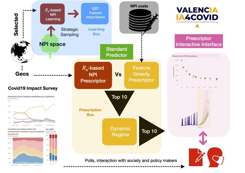
2         M.A. Lozano et al.

non-essential workplaces to requiring citizens to wear masks and limiting national
and/or international travel. How to model the impact that the applied NPIs
have on the progression of the pandemic is a non-trivial task, particularly for
traditional meta-population approaches. Moreover, the social and economic costs
of applying NPIs for a sustained period of time has led to the largest global
recession in history, with more than a third of the global population under confine-
ment during the first wave of the pandemic in March - April of 2020. The global
GDP shrunk by nearly 22 trillion of US dollars as of January 2021, according
to the IMF1 . Beyond the economic cost, the social cost of the pandemic is also
staggering, preventing children and teenagers from attending schools, cancelling
cultural activities and forbidding people to visit their friends or relatives.
    In view of these challenges, the XPRIZE foundation organized in November
of 2020 a global competition called the 500K XPRIZE Pandemic Response
Challenge sponsored by Cognizant [1]. This four-month challenge focused on
the development of data-driven AI systems to predict COVID-19 infection rates
and prescribe Non-pharmaceutical Intervention Plans that governments and
communities could implement to minimize harm when reopening their economies.
    In this paper, we describe the predictor and prescriptor models developed by
ValenciaIA4COVID, the winning team of the competition. The paper is organized
as follows: Section 2 provides an overview of the most relevant related work. The
data used in the competition is described in Section 3. The predictor and the
prescriptor models are presented in Section 4 and 5, respectively, followed by
the experimental results in Section 6. The main conclusions of our work and our
future lines of research are outlined in Section 7.

2     Related work

We built a COVID-19 infections predictor based on Long Short Term Memory
(LSTM) networks [13]. Here, we briefly provide an overview of the approaches that
are the most similar to ours, i.e. based on recurrent neural networks. Comparative
analyses with other methods can be found in e.g. [25].
    Chatterjee et al. [7] applied stacked, bidirectional LSTMs and compared
them with multilayer LSTMs. They obtained good accuracy in the prediction of
the total number of cases and deaths in the world. Moreover, they did not find
any statistical correlation between COVID-19 cases and temperature, sunshine,
and precipitation, showing that the number of infections mostly depends on the
behavior and density of the population. In [8], LSTMs were used to predict the
evolution of the pandemic in Canada and compared it with the USA, Spain, and
Italy. Prompt interventions were found to have a strong impact in minimizing
the total number of infections, though the accuracy of their predictions was good
only for a relatively short time period. Other examples of early works explored
using LSTMs to predict COVID-19 cases and the effect of NPIs in India [3] and
1
    https://www.dw.com/en/coronavirus-global-gdp-to-sink-by-22-trillion-over-covid-says-imf/a-
    56349323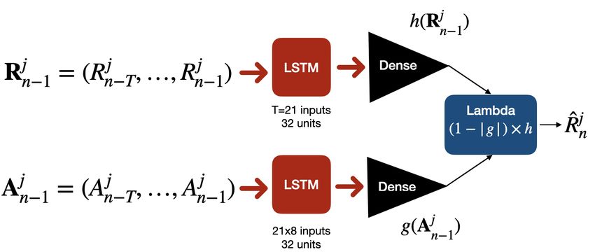
Open Data Science to fight COVID-19                 3

Iran [4], with accurate results within a prediction interval of one week up to a
month.
    Clustering algorithms have been used to improve the models’ performance. In
[19] the authors use an LSTM to predict cases in different states of Brazil. First,
they cluster nations by their temporal series of infections and then assign each
Brazilian state to the closest cluster. Global COVID-19 case data was also used
in [14] to cluster countries according to their outcomes.
    To the best of our knowledge, our work is the first to propose a bank of
LSTMs to predict the evolution of the coronavirus pandemic in 236 countries and
regions in the world, with good prediction results over a long time period (up to
180 days) and taking into consideration the NPIs applied in each country/region.
    Regarding the prescriptor part of our work, there are very few related ref-
erences. In [24] a multi-objective genetic algorithm was used to find optimal
policies using data from Wuhan. Sameni presents an approach to find a balance
between interventions and the number of cases with a core compartmental model.
This approach requires evaluating the impact of the policy on the evolution of
the disease [22]. Several works evaluated the effectiveness of NPIs: see [21,20]
for studies in Italy, Taiwan and Malaysia or [10,6] for recent studies in Europe.
Finally, Miikkulainen et al. propose a neuroevolution approach to identify a
Pareto-optimal set of NPIs [17], that was recommended during the Challenge.

3     Data

The coronavirus is the first global pandemic for which there is extensive data
captured and shared on a daily basis for most countries and regions in the world.
The Challenge leveraged publicly available official COVID-19 case data together
with the Oxford COVID-19 Government Response Tracker data set2 as the main
data sources to be used during the competition [11]. This data set provides
information for 186 countries and state/region-level data for the US, UK, Canada,
and Brazil. The Challenge considered 182 countries3 , the 50 US states and the 4
regions in the UK, yielding a total of 236 countries or regions. In the rest of the
paper, we will use GEO to denote the countries/regions.
    The available data sources can be split into case-related data, i.e. number
of daily confirmed COVID-19 cases, and action or NPI -related data, i.e. the
NPIs and their level of activation each day for each GEO. In the Challenge, we
considered 12 NPIs of two types: confinement-based and public health-based, that
are summarized with all their possible levels of activation in Table 1.

4     Predictors of COVID-19 cases

This part of the Challenge required building a predictor of the number of confirmed
COVID-19 cases in the 236 GEOs for up to 180 days into the future, and
2
    https://www.bsg.ox.ac.uk/research/research-projects/coronavirus-government-response-tracker
3
    Tonga, Malta, Turkmenistan and Virgin Islands- were not considered due to lack of reliable data.
4 M.A. Lozano et al.
Table 1. NPIs considered in the Challenge and their possible activation values. The
predictor is trained with confinement interventions (C1 to C8). Both confinement and
public health interventions (H1 to H3 and H6) are considered in the prescriptor.
NPI name Values NPI name Values
C1. School closing [0,1,2,3]
C7. Internal movement restrictions [0,1,2]
C2. Workplace closing [0,1,2,3]
C8. International travel controls [0,1,2,3]
C3. Cancel public events [0,1,2]
H1. Public information campaigns [0,1,2]
C4. Restrictions on gatherings [0,1,2,3]
H2. Testing policy [0,1,2,3]
C5. Close public transport [0,1,2]
H3. Contact tracing [0,1,2]
C6. Stay at home requirements [0,1,2,3]
H6. Facial coverings [0,1,2,3,4]
considering the different NPIs implemented in each GEO. Evidently, the NPIs
should impact the transmission of the disease and hence the number of cases. Next,
we summarize our notation, followed by a description of our deep learning-based
predictive model.
4.1 Notation
In the following, we will use the following terms and notation:
1. GEO: We denote as GEO a country or a region (e.g. California). We use the
index j to refer to each GEO.
2. Population (P j ): P j denotes the total population of GEO j. We assume
that each GEO’s population is constant during the entire period of time.
3. NewCases (Xnj ): The daily number of new cases on day n and GEO j is
denoted by Xnj . The first day considered is March, 11th 2020.
4. ConfirmedCases (Ynj ): The cumulative
Pn number of confirmed cases up to
day n in GEO j is given by Ynj = i=1 Xij .
5. SmoothedNewCases (Znj ): We compute the average number of new cases
1
PK−1 j
between days n − K + 1 and n in GEO j as Znj = K i=0 Xn−i . This prevents
noise due to different imputation policies (some GEOs do not report cases on
weekends, while others do). We use K = 7 to smooth over one week.
6. CaseRatio (Cnj ): The ratio of cases between two consecutive days is denoted
j
by Cnj = Znj /Zn−1 . It indicates the growth/decrease in the number of cases.
7. Susceptible Population (Snj ): The number of susceptible individuals to be
infected with coronavirus on day n and for GEO j is denoted by Snj .
8. ScaledCaseRatio (Rnj ): It is the CaseRatio Cnj divided by the proportion of
j
susceptible individuals in GEO j, Rnj = Cnj P j . It captures the effects of a finite
Sn
population, as it depends on proportion of susceptible individuals in GEO j.
9. Action (Ajn ): The vector with the applied NPIs in GEO j on day n.
j
10. Stringency of Ajn (StrA n
): The stringency of an NPI applied in GEO j on
j PH6
day n is given by StrAn = i=C1 ajn (i) · Costj (i), where Costj is the cost vector
of each of the 12 different types of NPIs ([C1...C8,H1,H2,H3,H6]) in GEO j.
11. Intervention Policy (IP): The sequence of daily 12-dimensional NPI orOpen Data Science to fight COVID-19 5
action vectors applied over a time period T .
12. Stringency of an Intervention Policy: The sum of the stringencies of
the NPIs or actions Ajn applied each day n over the time period T .
bnj is the estimated number new
We denote estimations with a b. symbol, e.g. X
j
cases and Rn the estimated scaled case ratio, both for GEO j and day n.
b
4.2 SIR Epidemiological Model
The predictors model the dynamics of the epidemics in each GEO j using an
underlying basic SIR compartmental meta-population model [2]. In this model,
the population is divided into three different states: S (Susceptible), Z (Infected),
and D (Removed, due to recovery or death). The dynamics of such an SIR model
is included in the S.M. The evolution of the number of infected individuals is
j
Sj j
given by dZ j
dt = β Pj Z − µZ , where β is the infection rate which controls the
probability of transition between the S and Z; and µ is the recovery or removal
rate, controlling the probability of transition between the Z and D states. When
j
discretizing dZdt for two consecutive days, we obtain
!
j Sj j j
j
Sn−1 j
Znj = Zn−1 + β n−1 Zn−1 − µZn−1 = 1+β − µ Zn−1 . (1)
Pj Pj
which yields
(1 − µ)Pj Znj P j
Rnj = +β = . (2)
Snj j
Zn−1 Snj
This equation links Rnj with the parameters of the SIR model. The larger the
Zj
Rnj , the larger Z j n and hence the larger the growth in the number of cases.
n−1
Given that µ is constant in (2), the larger the infection rate β, the larger the Rnj .
Moreover, the infection rate and thus Rnj depend on the applied NPIs.
bnj , we can estimate the number of cases for day n at GEO j:
If we predict R
j
!
bnj
X = bnj Sn−1
R j
− 1 KZn−1 j
+ Xn−K . (3)
Pj
where K = 7 is the size of the temporal window used to compute Zn . As previously
explained, Xn−K is the reported new cases for day n − K; R bnj is the predicted
j j j
Rn ; P is the population of GEO j; and Zn−1 is the cumulative number of cases
averaged over K days for day n − 1 in GEO j.
bnj given the data up to day
Thus, the goal of the predictors is to estimate R
j
n − 1. Since Rn depends on the transmission rate and the dependency of the
transmission rate on the NPIs, the predictors consider the number of COVID-19
infections (context) and the applied NPIs (actions) each day in each GEO.6 M.A. Lozano et al.
4.3 Baseline or standard predictor
The baseline or standard predictor was provided by the Challenge organizers [17].
It consists of two parallel LSTMs, one to model the context – given by the Rnj
– and the other to model the actions (Ajn ) applied on day n in GEO j. Figure
1 (left) depicts the architecture of this baseline model. It uses the context and
action data to get predictions separately, joining both outputs via a lambda
merge layer.
Fig. 1. Left: Baseline LSTM-based predictor; Right: ValenciaIA4COVID predictor.
The lambda layer combines the output of the context LSTM h (top) and
the output of the action LSTM g (down), represented in Figure 1. The input
to the LSTM h is the vector of values of Rn in the previous T days in GEO
j, namely Rjn−1 = (Rn−T
j j
, . . . , Rn−1 ). The input to the LSTM g is the matrix
of 12-dimensional NPIs (actions) taken during the previous T days in GEO j,
namely Ajn−1 = (Ajn−T , . . . , Ajn−1 ).
In our experiments we set T = 21, similarly to [17]. Such time window
mitigates the noise due to how different GEOs report cases (e.g. Spain does
not report confirmed cases during the weekends and holidays, France reports
just four days per week, etc.). Moreover, this temporal granularity enables the
model to consider the average period of 12-15 days between being exposed to the
coronavirus, being detected and tested as a new confirmed case [15].
The output of the lambda layer for day n is the predicted R bnj given by
bnj = f (Aj , Rj ) = (1 − g(Aj ))h(Rj )
R (4)
n−1 n−1 n−1 n−1
with g(Ajn−1 ) ∈ [0, 1] and h(Rjn−1 ) ≥ 0. More details about the baseline model
can be found in [17]. Note that when making predictions into the future, the
j
Rn−i values in the vector Rjn are replaced by the estimations provided by the
predictor, namely R bj , for n − i > currentd ay, i = 1, . . . , T .
n−iOpen Data Science to fight COVID-19 7
4.4 ValenciaIA4COVID (V4C) predictor
Similarly to the baseline predictor, we implemented an architecture with 2 LSTM-
based branches: a context branch, where we modeled the Rn time series and an
action branch, where we modeled the time series of the eight confinement-based
([C1...C8]) Non-pharmaceutical Interventions. While we did not consider public
health-based NPIs, we improved the baseline predictor in several ways. We denote
this improved model as the ValenciaIA4COVID or V4C predictor.
4.4.1. Context branch
We identified large variability in the time series of confirmed COVID-19 cases
depending on the GEO, which made it difficult for a single LSTM context model
to perform well everywhere. More precisely, the analysis of the weights of a single
model trained on all the data showed that the LSTM matrices were full rank.
Hence, we opted for a bank of LSTM context models, shown in Figure 1 (right).
Bank of context models We created the bank as follows: First, we clustered
the GEOs via a K-means algorithm applied to the time series of reported number
of COVID-19 cases per 100K inhabitants. We optimized the number of clusters
using the Elbow method, obtaining 15 different clusters shown in the S.M.
Next, we trained a reference LSTM model with data from the 20 most-affected
GEOs and 15 different cluster LSTM models using data from all the GEOs in
each of the 15 clusters. In our experiments, we set March 11th, 2020 as the
starting date for training the models. We then evaluated the reference and all the
cluster models on our testing data for all the GEOs. Our testing period started on
Nov. 1st for long-term evaluation and Dec. 1st for short-term evaluation, ending
on Dec. 21st, 2020. We automatically selected the model with the lowest MAE
per 100K inhabitants in each GEO, applying Occam’s razor principle to minimize
the number of models in our bank. Thus, we favored the reference model when it
obtained a similar performance to the best of the cluster models. As a result of
this process, we selected nine models: the reference model, applied in 135 GEOs;
and eight cluster models applied in the remaining GEOs. A visualization of the
cluster and model assignments can be found here4 .
LSTMs Architecture. In the context branch (h) we implemented two
different LSTM-based architectures, as depicted in Figure 1 (right): one for
the reference model and the other for each of the eight cluster models. The
reference model includes a convolutional layer with ReLu activation function and
a bidirectional LSTM followed by a dense layer. Each convolutional layer has 64
filters of size 8. This reference model empirically generalized well for 135 GEOs.
The cluster models consist of a stacked version of the architecture of the
reference model, with two convolutional layers and two stacked bidirectional
LSTMs. Each convolutional layer also has 64 filters of size 8 with ReLu as the
activation function and add a final dense layer. After the double 1D convolution
spans the characterization of the input sequence, the first LSTM encodes such
a characterization in states of 64 dimensions (bidirectional) and feeds into the
4
https://tinyurl.com/cjstz4yc8 M.A. Lozano et al.
second LSTM, whose units can now operate at a different time scale. This added
complexity enabled the models to perform well in the GEOs where the reference
model did not. After model selection, we obtained a bank of eight different cluster
models.
4.4.2. Action branch
We used an LSTM followed by two dense layers to smooth the output and
hence better capture non-linearities. Similarly to [17], we used a sigmoid activation
function to guarantee that the action layer’s output to be in [0,1]. Since increasing
the activation or stringency of an NPI should not decrease its effectiveness, g is
constrained to satisfy the condition: if min(A − A0 ) ≥ 0 −→ g(A) ≥ g(A0 ). This
constraint is enforced by setting all trainable parameters of g to be non-negative
(absolute value) after each parameter update. Note that convolution here is not
considered in order to keep the raw NPI constraints. The V4C predictor only
considers the confinement NPIs, so each Ajn is an 8-dimensional vector with the
level of activation of the eight confinement NPIs (see Table 1).
4.4.3. Merge function
The two branches use the data from the last 21 days that are combined into
a final dense layer to get the predicted R bn . The outputs of each branch (h and
g) are merged by the lambda function defined in (4). Thus, the predicted R bn
provided by the context branch is modified by the output from the action branch.
The stricter the NPIs, the larger the output from the action layer, thus reducing
the context layer’s output. Finally, once the model gives the predicted R bn , the
predicted number of new infections for day n, X bn , is obtained using (3).
5 Prescriptor of Intervention Policies
The final phase of the XPRIZE competition required building a prescriptor which
would recommend for each GEO and for any period of time, up to 10 different
Intervention Policies (IP) with the best balance between their economic/social
cost and the resulting number of COVID-19 cases.
Thus, it entailed solving a two-objective optimization problem by identifying
the set of solutions that would be on the Pareto front [5,16,17]. On the one hand,
there is the stringency of a certain IP which captured the sum of the costs of
implementing such a policy. On the other hand, there is the number of COVID-19
cases per 100K inhabitants which would result from applying such IP. Given that
this is a hypothetical scenario, the number of COVID-19 infections under the IPs
was estimated by the baseline or standard predictor provided by the XPRIZE
Challenge organizers. All the teams used the same predictor to enable the judges
to compare the prescriptors from different teams properly.
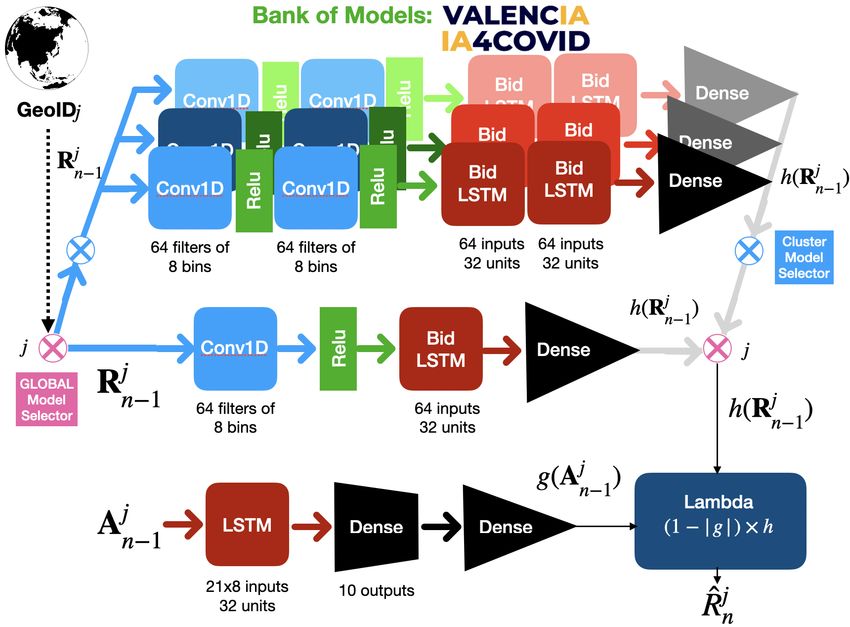
Our goal in the Prescription phase of the competition was to develop an
interpretable, data-driven and flexible prescription framework that would be
usable by non machine-learning experts, such as citizens and policymakers in the
Valencian Government. Our design principles were therefore driven by developing
explainable and transparent models. The Challenge entailed finding the set
of Pareto-optimal IPs with the best trade-off between their economic/socialOpen Data Science to fight COVID-19 9
Fig. 2. V4C Prescriptor. The (offline) learning box (in blue) infers the convergence R
bn
for the sampled NPIs, and the Gradient Boosted Trees identify the feature importance.
The prescriptor relies on the standard XPRIZE predictor. The first set of NPIs is
obtained by the NPI-R bn mapping; the second set, using a feature importance-based
greedy algorithm. These two sets compete and up to 10 non-dominated IPs are selected.
costs and their associated number of resulting COVID-19 cases. An intervention
policy IP1 dominates another intervention policy IP2 if the stringency(IP1 ) ≤
stringency(IP2 ) and the resulting number of COVID-19 cases under IP1 < than
under IP2 . The goal was to find up to 10 IPs for each GEO, for any time period
and any costs that would dominate the rest of possible IPs. As in the case of
our predictor, we decided to combine complementary approaches to have a more
robust solution, shown in Figure 2.
5.1 Modeling the NPI - COVID-19 cases space
Before building the prescriptor, we performed an exploratory data analysis of
the problem space. Our goal was to shed light on the relationship between the
NPIs and the resulting number of COVID-19 cases. Considering all the possible
values of each dimension of the NPI or action vector, there are 7,776,000 possible
combinations of NPI vectors that could be applied at each time step.
Each NPI vector, when applied for a minimum amount of time, would lead to
a reduction or increase in the number of COVID-19 cases in the GEO where it is
applied (see Equation 4). To better understand the impact that different NPI
vectors have on the number of COVID-19 cases, we ran numerous experiments
where we called the predictor with different values of the NPI vector over varying
time periods of 30 to 90 days and on a sample of 21 representative GEOs from
different continents5 , namely: United States, Brazil, India, Mexico, Italy, China,
United Kingdom, France, England, Russia, Iran, Spain, Argentina, Colombia,
New York State, Peru, Germany, Poland, South Africa, Texas and California.
For each case, we obtained the resulting R bn estimated by the predictor.
In our experiments, we observed that the same NPI vector would lead
to the same convergence R bn in all the GEOs and over any time period
provided that the NPI was applied for long enough (see a justification in the S.M.).
5
We selected amongst the most affected countries and regions across the globe.10 M.A. Lozano et al.
Moreover, we found that the convergence time of R bn is inversely proportional to
its value. As per Eq. (2), note that the larger the Rbn , the larger the number of
resulting COVID-19 cases. We refer to this finding as the Rn synchronization
principle. Moreover, all countries underwent a transitory period of ≈ 21 days
since the application of a certain NPI before their R
bn started converging towards
its convergence value. Figure 3 illustrates the convergence of the R bn for two
different NPI vectors in the 21 selected GEOs.
5.2 Prescriptors
5.2.1. Prescriptor Method 1: Rn -based NPI selection
Based on the Rn synchronization principle, one could easily obtain the Pareto-
optimal front of intervention policies if the mapping between the 7.8 million of
possible combinations of the NPI vector and their associated convergence R bn
were to be known. Unfortunately, generating such a mapping was not feasible in
the time frame provided by the Challenge as it would require making millions of
calls to the predict function. Hence, we opted for computing a sample of such a
matrix (whose distribution is shown in the S.M.), obtained as (1) all the NPI
vectors with stringencies [0 to 6] and [28 to 34]; (2) all NPI vectors with one and
two non-zero entries; and (3) a random sample of 10,000 NPIs.
For each NPI in the sample, we computed the convergence R bn , and the
resulting total number of COVID-19 cases in 20 and 60 days.
Using this NPI-Rbn matrix, we trained state-of-the-art machine-learning models
to predict the Rn for any given NPI vector. The best performing and explainable
b
model were Gradient Boosted Trees, which obtained a MAE on the test set of
0.0003. While such MAE was still too large for us to be able to fill-in all the
missing elements in the NPI-R bn matrix, we carried out a feature importance
analysis and discovered that the C2, C1, H2, C4 and C5 interventions are, in this
order, the most important to predict their associated R bn and hence the resulting
number of COVID-19 cases (see S.M. for details).
Thus, we also included in our NPI-R bn matrix all the NPI vectors with non-
zero values in their C1, C2, C4, C5 and H2 interventions and zero in the rest of
the dimensions. This led to a total of 54,652 NPI vectors.
As a result, we generated a matrix with the mapping between these different
NPI vectors, their associated stringencies (at cost 1), the number of cases that
they would lead to at 20 days and at 60 days, and their convergence R bn . We
carried out all computations on the sample of 21 previously listed GEOs.
At run time, given an input cost vector, the prescriptor computes the strin-
gency of each row in the NPI-R bn matrix and identifies the NPI combinations
that are on the Pareto front by selecting those that lead to the best trade-off
between their stringencies, their associated number of cases at 20 and 60 days
and their convergence R bn . More details are included in the S.M.
5.2.2. Prescriptor method 2: Feature greedy NPI selection
As per the feature importance analysis described above and given a cost vector,
we developed a greedy NPI prescriptor as follows: each dimension of the NPIOpen Data Science to fight COVID-19 11
Fig. 3. Rˆn convergence for two different NPI vectors on 21 representative GEOs.
vector is ranked by its priority, computed as its feature importance divided by its
cost. This prescriptor consists of a greedy algorithm that consecutively activates
to its maximum value each NPI dimension by order of its priority. This method is
related to the greedy strategies developed to solve the knapsack problem6 . 5.2.3.
Prescriptor combination
Each of the methods above provides a set of NPI recommendations for each
GEO for each day. From such a set, we select the 10 best NPIs that satisfy the
following criteria: (1) they are not dominated by any other NPI; and (2) they
contribute to having a diverse set of NPIs that cover the full range of possible
stringency values. Additional details are included in the S.M.
5.3 Intervention policy definition
Finally, the prescriptor needs to provide a set of up to 10 Intervention Policies, i.e.
dynamic regimes of applying the selected NPIs over the time period of interest. To
do so, we compute all possible combinations of subsequently applying the selected
NPIs in chunks of minimum 14 days (to enable the NPIs to act) and identify the
Pareto-front set of combinations that would yield the optimal trade-off between
stringency and number of cases. The total number of chunks is dynamically
determined. From this set of combinations, we again select the 10 that (1) are not
dominated by any other policy; (2) contribute to having a diverse set of policies
along the stringency axis and (3) minimize the changes in NPIs, as every NPI
change has a social cost from a practical perspective.
Two screenshots of the interactive visualization that we developed so policy-
makers could easily compare the prescribed IPs are shown in the S.M. and can
be found here7 .
6 Experimental results
In this Section, we report the results of quantitatively evaluating our predictor
both in short and long-term prediction scenarios and qualitatively assessing
6
See https://en.wikipedia.org/wiki/Knapsack problem.
7
https://public.tableau.com/app/profile/kristina.p8284/viz/PrescriptionsWeb/Visualize12 M.A. Lozano et al.
the performance of our predictor and prescriptor in hypothetical scenarios. Our
source code is publicly available8 .
6.1 Predictor
We evaluated the predictive performance of our COVID-19 cases predictor and
compared it to the baseline model under different scenarios. We computed both
the Mean Absolute Error (MAE) of the estimated number of COVID-19 cases
per 100K inhabitants for each GEO in the Challenge and the Mean Rank of our
model when compared to the baseline model.
All the models were trained with data from the Oxford COVID-19 Government
Response Tracker dataset, from March 11th to December 17th 2020, for the 20
most affected countries in terms of confirmed cases.
40M
XPRIZE baseline model XPRIZE baseline model XPRIZE baseline model
V4C model 3M V4C model 800k V4C model
Daily new cases 7-day average
Daily new cases 7-day average
Daily new cases 7-day average
30M 2.5M
600k
2M
20M
400k
1.5M
10M
200k
1M
0 0.5M
0
03 17 31 14 28 14 28 11 25 09 23 06 03 17 31 14 28 14 28 11 25 09 23 06 03 17 31 14 28 14 28 11 25 09 23 06
Jan Feb Mar Apr May Jun Jan Feb Mar Apr May Jun Jan Feb Mar Apr May Jun
Date Date Date
Fig. 4. Smoothed predicted daily new cases worldwide (7-day average) for three different
future scenarios based on different values of the NPI vector: zero (left), frozen (center)
and maximal (right) NPIs applied. Note how without any NPIs there is a large wave of
infections, which is avoided when the NPIs set to their maximal values.
As the consistency of the model is an important characteristic to assess, we
evaluated the models both in short-term and long-term predictions. Short-term
evaluations consisted in generating predictions for 3 weeks ahead into the future
for the time period between Dec 1st and Dec 21st, 2020. Long-term evaluations
were two-fold: First, with historic data, we tested the predictions between Nov 1st
and Dec 21st, 2020; Second, we ran the predictors under three different 180-day
prediction scenarios: (i) a scenario where the NPIs were frozen as of their values
in Dec 21st 2020; (ii) a scenario with all NPIs in all GEOs were set to their
maximum levels; and (iii) a scenario where all NPIs in all GEOs were set to 0.
The behavior of our model under these three conditions made intuitive sense, as
depicted in Figure 4.
Table 2 displays the MAE per 100K inhabitants and the Mean Rank of the
proposed model when compared to the baseline model provided by the XPRIZE
organizers. We also include the results of only using our reference context model
without the clusters. As seen on the Table, our model outperforms the baseline
model in all evaluation scenarios in terms of MAE and Mean Rank. Moreover,
8
https://github.com/malozano/valencia-ia4covid-xprizeOpen Data Science to fight COVID-19 13
during the predictor evaluation phase of the XPRIZE Challenge, our predictor
ranked third in the world in Mean Rank amongst all the teams, first in Mean Rank
in Asian and in European GEOs. As per our collaboration with the President
Table 2. Predictor results in short and long-term evaluations in the 236 GEOS.
Short-term Long-term
Predictor
MAE Mean Rank MAE Mean Rank
XPRIZE LSTM baseline 157.924142 2.106383 935.340780 2.297872
V4C (w/o clusters) 138.208982 2.144681 825.375377 1.834043
V4C with clusters 126.331216 1.748936 803.587381 1.868085
of the Valencian Government in Spain, we were able to share the predictions of
our predictor during the 3rd wave of the COVID-19 pandemic that started right
after Christmas of 2020. Figure 5 shows the predictions of our model (blue) when
compared to the baseline predictor (red) and the ground truth (yellow). As seen
in the Figure, our predictor was very accurate in predicting the evolution of the
pandemic while taking into account the different NPIs that were implemented at
the time. It provided valuable input to the Government in their decision-making.
6.2 Speed and Resource Use
In terms of training, we used an Intel Core i7 with 256 Gb RAM and GPU. The
training time of the reference model with 20 trials was 108 minutes and of the
cluster models ranged between 24 minutes (largest cluster with 106 GEOs) and
44 seconds (smallest cluster with 2 GEOs).
We carried out our prediction experiments on an Intel Core i7, 4 cores, 2,7
Ghz, 16GB 2133MHz LPDDR3. Table 3 (Top) summarizes the times needed to
14k
Ground Truth 12k Ground Truth
12k XPRIZE standard model XPRIZE standard model
Daily new cases 7-day average
V4C model 10k V4C model
10k
Daily new cases
8k
8k
6k
6k
4k
4k
2k 2k
0 0
06 13 20 27 03 10 17 24 31 07 14 21 28 07 14 21 28 06 13 20 27 03 10 17 24 31 07 14 21 28 07 14 21 28
Dec Jan Feb Mar Dec Jan Feb Mar
Date Date
Fig. 5. Predictions vs ground truth for the Valencian region (Spain) during the third
wave: daily new cases (left) and smoothed daily new cases (right).
produce a prediction for all the GEOs by the baseline model and our proposed14 M.A. Lozano et al.
Table 3. Top: Total time needed to generate predictions for all the GEOs. Bottom:
Prescriptor results: # of dominating / # of dominated prescriptions for 5-day (from
Aug 1st to Aug 5th, 2020), 31-day (from Jan 1st to Jan 31st, 2021) and 90-day (from
Jan 1st to Mar 31st, 2021) time periods.
Window size of prediction
Predictor 31-days 61-days 180-days
Baseline 212 seconds 409 seconds 1,092 seconds
V4C 417 seconds 597 seconds 1,239 seconds
Prescriptor 31-days 61-days 180-days
Greedy 127 / 1814 130 / 1829 163 / 1839
Feature greedy 921 / 114 930 / 117 986 / 163
V4C prescriptor 927 / 47 934 / 48 986 / 137
model for three different sizes of the prediction period. As seen on the Table, the
computation needs of our model were well below the maximum time allowed in
the XPRIZE competition (60 minutes). We favored simplicity in our design and
aimed to minimize the energy consumption to be as planet-friendly as possible.
6.3 Prescriptor
Given the hypothetical nature of the prescriptor, we were not able to quantita-
tively evaluate its performance against ground truth. However, we did carry out
domination tests between the IPs recommended by our model when compared to
a greedy algorithm for the 236 GEOs in the Challenge and under both unitary
and random costs policies for a time period of 60 days into the future. Figure 6
depicts the recommended IPs by our model (orange and green) when compared
to a greedy prescriptor (blue).
Table 3 (bottom) shows the number of times the IPs recommended by our
prescriptor dominated and were dominated by the IPs suggested by the greedy
approach for all GEOs. Moreover, our prescriptor provided the IP recommenda-
tions in under 2 hours for all GEOs in the Challenge, well below the maximum
allowed limit of 6 hours.
BlindGreedy BlindGreedy 50000 BlindGreedy
V4C V4C V4C
2000 FeatGreedy FeatGreedy FeatGreedy
9000 45000
1950
Mean cases per day per geo
Mean cases per day per geo
Mean cases per day per geo
40000
8000
1900 35000
7000 30000
1850
25000
1800 6000
20000
1750 15000
5000
0 5 10 15 20 25 0 5 10 15 20 25 30 0 5 10 15 20 25 30
Mean stringency Mean stringency Mean stringency
Fig. 6. Number of cases vs stringency obtained from prescriptions generated for 5 days
(left), 31 days (center) and 90 days (right).Open Data Science to fight COVID-19 15
7 Conclusions and Future Work
In this paper, we have described the models developed by the winning team
of the 500K XPRIZE Pandemic Response Challenge. The competition entailed
first developing a model to predict the number of COVID-19 cases in 236 coun-
tries/regions in the world, for up to 180 days into the future and considering
the Non-pharmaceutical Interventions deployed in each country/region. In this
phase, we developed an LSTM-based bank of models which outperformed the
baseline model provided by the Challenge organizers and yielded the third best
Mean Rank amongst all the teams in the competition. The proposed model was
successfully used by the President of the Valencian government in Spain during
the third wave of COVID-19 infections in December - February 2021.
Next, the teams were asked to develop a prescription model that would
recommend up to 10 Intervention Policies (IPs) in each of the 236 GEOs in the
world for any time period and costs that would achieve the best trade-off between
the total cost of the IP and the resulting number of coronavirus infections.
Our winning solution leveraged the Rn synchronization principle to provide
Pareto-optimal IPs that clearly dominated other approaches.
We believe that this work contributes to the necessary transition to more
evidence-driven policy-making, particularly during a pandemic. Future lines
of work include developing the intervention prescriptor within the Valencian
Government, developing a theoretical proof of the Rn synchronization principle
and including the impact of vaccinations in our model.
Acknowledgements The authors have been partially supported by grants
FONDOS SUPERA COVID-19 Santander-CRUE (CD4COVID19 2020–2021),
Fundación BBVA for SARS-CoV-2 research (IA4COVID19 2020-2022) and the
Valencian Government. We thank the University of Alicante’s Institute for Com-
puter Research for their support with computing resources, co-financed by the
European Union and ERDF funds through IDIFEDER/2020/003. MAGM ac-
knowledges funding from MEFP Beatriz Galindo program (BEAGAL18/00203).
References
1. 500k XPRIZE Pandemic Response Challenge, sponsored by Cognizant, https:
//www.xprize.org/challenge/pandemicresponse
2. Allen, L.: Some discrete-time SI, SIR, and SIS epidemic models. Math. Biosci.
124(1), 83–105 (1994)
3. Arora, P., Kumar, H., Panigrahi, B.K.: Prediction and analysis of covid-19 positive
cases using deep learning models: A descriptive case study of india. Chaos, Solitons
& Fractals 139, 110017 (2020)
4. Ayyoubzadeh, S., Ayyoubzadeh, S., Zahedi, H., Ahmadi, M., Kalhori, S.: Predicting
COVID-19 incidence through analysis of Google trends data in Iran: data mining
and deep learning pilot study. JMIR Public Health Surveill. 6(2) (2020)
5. Belakaria, S., Deshwal, A., Doppa, J.: Max-value entropy search for multi-objective
bayesian optimization. In: Wallach, H., Larochelle, H., Beygelzimer, A., d'Alché-Buc,
F., Fox, E., Garnett, R. (eds.) NeurIPS. vol. 32 (2019)16 M.A. Lozano et al.
6. Brauner, J.M., Mindermann, S., Sharma, M., et al.: Inferring the effectiveness of
government interventions against COVID-19. Science 371(6531) (2021)
7. Chatterjee, A., Gerdes, M., Martinez, S.: Statistical explorations and univariate
timeseries analysis on COVID-19 datasets to understand the trend of disease
spreading and death. Sensors 20(11), 3089 (2020)
8. Chimmula, V.K.R., Zhang, L.: Time series forecasting of covid-19 transmission in
canada using LSTM networks. Chaos, Solitons & Fractals 135, 109864 (2020)
9. Ferguson, N., Cummings, D., Cauchemez, S., et al: Strategies for containing an
emerging influenza pandemic in Southeast Asia. Nature 437(7056), 209–214 (2005)
10. Flaxman, S., Mishra, S., Gandy, A., et al: Estimating the effects of non-
pharmaceutical interventions on Covid-19 in Europe. Nature 584, 257—-261 (2020)
11. Hale, T., Angrist, N., Goldszmidt, R., Kira, B., et al.: A global panel database of
pandemic policies (Oxford COVID-19 Government Response Tracker). Nat. Hum.
Behav. pp. 1–10 (2021)
12. Hethcote, H.: The mathematics of infectious diseases. SIAM Rev. 42(4), 599–653
(2000)
13. Hochreiter, S., Schmidhuber, J.: Long short-term memory. Neural Comput. 9(8),
1735–1780 (1997)
14. Khan, M., Hossain, A.: Machine learning approaches reveal that the number of
tests do not matter to the prediction of global confirmed COVID-19 cases. Front.
Artif. Intell. Appl. 3, 90 (2020)
15. Lauer, S., Grantz, K., Bi, Q., Jones, F., et al: The incubation period of coronavirus
disease 2019 (COVID-19) from publicly reported confirmed cases: estimation and
application. Ann. Intern. Med. 172(9), 577–582 (2020)
16. Lu, Z., Whalen, I., Dhebar, Y., Deb, K., et al.: NSGA-Net: Neural architecture
search using multi-objective genetic algorithm (extended abstract). In: Bessiere, C.
(ed.) Proc. of the 29th Int. J. Conf. on AI, IJCAI-20. pp. 4750–4754 (2020)
17. Miikkulainen, R., Francon, O., Meyerson, E., Qiu, X., et al.: From prediction to
prescription: Evolutionary optimization of nonpharmaceutical interventions in the
COVID-19 pandemic. IEEE Trans. Evol. Comput. 25(2), 386–401 (2021)
18. Pastor-Satorras, R., Castellano, C., Van Mieghem, P., Vespignani, A.: Epidemic
processes in complex networks. Rev. Mod. Phys. 87, 925–979 (Aug 2015)
19. Pereira, I., Guerin, J., Silva J., A.G., Garcia, G., Piscitelli, P., Miani, A., Distante, C.,
Gonçalves, L.: Forecasting COVID-19 dynamics in Brazil: a data driven approach.
Int. J. Environ. Res. Public Health 17(14), 5115 (2020)
20. Rahman, M., Zaman, N., Asyhari, A., Al-Turjman, F., et al: Data-driven dynamic
clustering framework for mitigating the adverse economic impact of COVID-19
lockdown practices. Sustain. Cities Soc. 62, 102372 (2020)
21. Riccardi, A., Gemignani, J., Fernández-Navarro, F., Heffernan, A.: Optimisation
of non-pharmaceutical measures in COVID-19 growth via neural networks. IEEE
Trans. Emerg. Topics Comput. 5(1), 79–91 (2021)
22. Sameni, R.: Model-based prediction and optimal control of pandemics by nonphar-
maceutical interventions. arXiv preprint arXiv:2102.06609 (2021)
23. Tayarani, N., Mohammad, H.: Applications of artificial intelligence in battling
against COVID-19: A literature review. Chaos, Solitons & Fractals p. 110338 (2020)
24. Yousefpour, A., Jahanshahi, H., Bekiros, S.: Optimal policies for control of the
novel coronavirus disease outbreak. Chaos, Solitons & Fractals 136 (2020)
25. Zeroual, A., Harrou, F., Dairi, A., Sun, Y.: Deep learning methods for forecasting
COVID-19 time-series data: A comparative study. Chaos, Solitons & Fractals 140
(2020)You can also read