OCEANFILMS (Organic Compounds from Ecosystems to Aerosols: Natural Films and Interfaces via Langmuir Molecular Surfactants) sea spray organic ...
←
→
Page content transcription
If your browser does not render page correctly, please read the page content below
Research article
Atmos. Chem. Phys., 22, 5223–5251, 2022
https://doi.org/10.5194/acp-22-5223-2022
© Author(s) 2022. This work is distributed under
the Creative Commons Attribution 4.0 License.

       OCEANFILMS (Organic Compounds from Ecosystems to
         Aerosols: Natural Films and Interfaces via Langmuir
          Molecular Surfactants) sea spray organic aerosol
        emissions – implementation in a global climate model
                       and impacts on clouds
              Susannah M. Burrows1 , Richard C. Easter1 , Xiaohong Liu2 , Po-Lun Ma1 , Hailong Wang1 ,
                      Scott M. Elliott3 , Balwinder Singh1 , Kai Zhang1 , and Philip J. Rasch1,4
                           1 Pacific
                                   Northwest National Laboratory, Richland, Washington, USA
                                   2 Texas
                                        A&M University, College Station, Texas, USA
                           3 Los Alamos National Laboratory, Los Alamos, New Mexico, USA
                   4 Department of Atmospheric Sciences, University of Washington, Seattle, WA, USA

                         Correspondence: Susannah M. Burrows (susannah.burrows@pnnl.gov)

                                   Received: 24 January 2018 – Discussion started: 24 May 2018
                        Revised: 7 December 2021 – Accepted: 15 January 2022 – Published: 21 April 2022

      Abstract. Sea spray aerosol is one of the major sources of atmospheric particulate matter globally. It has in-
      creasingly been recognized that organic matter derived from ocean biological precursors contributes signifi-
      cantly to the composition of submicron sea spray and may modify sea spray aerosol impacts on clouds and
      climate. This paper describes the implementation of the OCEANFILMS (Organic Compounds from Ecosystems
      to Aerosols: Natural Films and Interfaces via Langmuir Molecular Surfactants) parameterization for sea spray
      organic aerosol emissions in a global Earth system model, the Energy Exascale Earth System Model (E3SM).
      OCEANFILMS is a physically based model that links sea spray chemistry with ocean biogeochemistry using a
      Langmuir partitioning approach. We describe the implementation details of OCEANFILMS within E3SM, com-
      pare simulated aerosol fields with observations, and investigate impacts on simulated clouds and climate. Four
      sensitivity cases are tested, in which organic emissions either strictly add to or strictly replace sea salt emis-
      sions (in mass and number) and are either fully internally or fully externally mixed with sea salt. The simulation
      with internally mixed, added organics agrees reasonably well with observed seasonal cycles of organic matter in
      marine aerosol and has been selected as the default configuration of the E3SM. In this configuration, sea spray
      organic aerosol contributes an additional source of cloud condensation nuclei, adding up to 30 cm−3 to South-
      ern Ocean boundary-layer cloud condensation nuclei concentrations (supersaturation = 0.1 %). The addition of
      this new aerosol source strengthens shortwave radiative cooling by clouds by −0.36 W m−2 in the global annual
      mean and contributes more than −3.5 W m−2 to summertime zonal mean cloud forcing in the Southern Ocean,
      with maximum zonal mean impacts of about −4 W m−2 around 50–60◦ S. This is consistent with a previous top-
      down, satellite-based empirical estimate of the radiative forcing by sea spray organic aerosol over the Southern
      Ocean. Through its mechanistic approach, OCEANFILMS offers a path towards improved understanding of the
      feedbacks between ocean biology, sea spray organic matter, and climate.

Published by Copernicus Publications on behalf of the European Geosciences Union.
5224                                       S. M. Burrows et al.: OCEANFILMS MOA: implementation and climate sensitivity

1   Introduction and motivation                                   1.1   Existing model parameterizations of MOA emissions

It has long been noted that organic matter constitutes a sub-     Several previous studies have proposed and implemented
stantial portion of submicron marine aerosol mass (Hoffman        representations of MOA emissions within a global climate
and Duce, 1974, 1976, 1977; Duce et al., 1983; Oppo et al.,       model, with variations in the emission representation and
1999). However, it has only recently been widely appreciated      the assumed aerosol microphysical properties. Most of these
that water-insoluble organic matter (WIOM) contributes sub-       studies were based on aerosol chemistry observations taken
stantially to submicron marine aerosol downwind of strong         primarily from two sites, at Mace Head, Ireland, and at Am-
seasonal phytoplankton blooms (O’Dowd et al., 2004) and           sterdam Island, in the Southern Ocean (Sciare et al., 2009;
has the potential to affect the number and chemical character     Rinaldi et al., 2013). O’Dowd et al. (2008) proposed an early
of aerosol and cloud condensation nuclei (CCN) in certain         parameterization for MOA emissions, which was later mod-
marine regions (McCoy et al., 2015).                              ified by Langmann et al. (2008) for inclusion in a global
   Although organic matter in ambient sea spray can also          model and further updated and evaluated by Vignati et al.
arise from condensation of volatile organic compounds (i.e.,      (2010) (which also corrects a typographical error in the for-
secondary organic aerosol), a large body of experimental ev-      mulation as printed in Langmann et al., 2008). In this ap-
idence shows that nascent sea spray also contains organic         proach, the organic mass fraction (OMF), defined as the ra-
matter of biogenic origin. Experiments using physical sim-        tio of MOA mass to the total of MOA and sea salt aerosol
ulations of the sea spray aerosol production process have         (SSA) mass, depends linearly on chlorophyll a [Chl a], with
shown that organic matter is co-emitted into sea spray aerosol    an imposed upper bound corresponding to the highest ob-
together with salt (Keene et al., 2007; Facchini et al., 2008a;   served values of OMF. Rinaldi et al. (2013) further updated
Gao et al., 2012; Bates et al., 2012; Schmitt-Kopplin et al.,     this parameterization by adding a linear dependence of OMF
2012; Ault et al., 2013; Prather et al., 2013; Quinn et al.,      on wind speed. This study also showed that the correlation
2014; Frossard et al., 2014a; Long et al., 2014; Alpert et al.,   between upwind [Chl a] and OMF was improved when a
2015; Kieber et al., 2016). The primary sea spray origin of       time lag of 8–10 d was introduced.
marine organic matter is also supported by laboratory stud-          Gantt et al. (2011) proposed an emission parameterization
ies and field experiments using a variety of analytical meth-     in which OMF depends on wind speed and [Chl a] by fitting
ods (see the review by Frossard et al., 2014b), which show        a nonlinear equation form to observed OMF at Mace Head,
that the chemical composition of submicron marine aerosol         Ireland, and Point Reyes, California. Meskhidze et al. (2011)
is similar to material drawn from the sea surface microlayer      further evaluated this parameterization and compared it to
(Facchini et al., 2008b; Leck and Bigg, 2005; Russell et al.,     Vignati et al. (2010), concluding that both parameterizations
2010).                                                            captured the magnitude of MOA concentrations, with Gantt
   Clouds in remote marine areas are particularly sensitive       et al. (2011) attaining better seasonality.
to changes in aerosol concentrations (Karydis et al., 2012;          Long et al. (2011) proposed another alternative approach
Moore et al., 2013), because cloud droplet number concen-         in which OMF depends nonlinearly on [Chl a], using the
trations (CDNCs) respond to perturbations in aerosol more         functional form of the Langmuir isotherm to drive the re-
strongly when background aerosol concentrations are low           lationship and using a fit to observed [Chl a] and OMF from
(Pringle et al., 2012). These clouds, located in regions where    two sea spray generation experiments to constrain the model
anthropogenic aerosols are scarce, are primarily influenced       parameters. The parameterization also takes particle diame-
by natural aerosol sources (Hamilton et al., 2014), and the       ter into consideration.
ability to constrain climate sensitivity using historical cli-       Additional model studies of MOA have largely built upon
mate records is in part limited by quantification of these nat-   these initial proposed parameterizations and further explored
ural sources (Karydis et al., 2012; Carslaw et al., 2013; Re-     their uncertainties, their sensitivities to certain aspects of the
gayre et al., 2020). Recent research also suggests that sea       model implementation, and the resulting implications for cli-
spray organic aerosol (which we abbreviate as MOA, for            mate. These studies have emphasized uncertainties in the
marine organic aerosol) can serve as nuclei for freezing of       choice to either add to or replace existing sea salt (Westervelt
cloud droplets (Knopf et al., 2011; Wilson et al., 2015; De-      et al., 2012), to assume that aerosols are internally versus ex-
Mott et al., 2016) and may play an important role as at-          ternally mixed (Meskhidze et al., 2011), and in the sea spray
mospheric ice nuclei in remote marine regions (Schnell and        fine-mode particle size (Tsigaridis et al., 2013).
Vali, 1975, 1976; Burrows et al., 2013a; Wilson et al., 2015;
Vergara-Temprado et al., 2017; McCluskey et al., 2019; Zhao
                                                                  1.2   Estimates of global annual MOA emissions
et al., 2021).
                                                                  The best estimates for global emissions of primary marine or-
                                                                  ganic matter (OM) from different model studies span a range
                                                                  from at least 2.8 to 76 Tg yr−1 (fine-mode emissions) and
                                                                  from 4.5 to 34.9 Tg yr−1 (coarse-mode emissions) (Spracklen

Atmos. Chem. Phys., 22, 5223–5251, 2022                                             https://doi.org/10.5194/acp-22-5223-2022
S. M. Burrows et al.: OCEANFILMS MOA: implementation and climate sensitivity                                                 5225

et al., 2008; Gantt et al., 2009; Vignati et al., 2010; Myrioke-    tems. In an effort to provide a path forward, Elliott et al.
falitakis et al., 2010; Ito and Kawamiya, 2010; Long et al.,        (2014) proposed the prospect of an approach based on un-
2011; Gantt et al., 2011; Myriokefalitakis et al., 2010; West-      derstanding of ocean surface films, and Burrows et al. (2014)
ervelt et al., 2012; Tsigaridis et al., 2013). These studies used   introduced a new framework for modeling the functional re-
both different emission parameterizations and different host        lationships between ocean biogeochemical variables and the
model systems (e.g., with differences in aerosol parameter-         composition of emitted sea spray particles, called OCEAN-
izations and atmospheric physics parameterizations impact-          FILMS (Organic Compounds from Ecosystems to Aerosols:
ing transport and removal), which are likely to also cause          Natural Films and Interfaces via Langmuir Molecular Sur-
differences in the simulated atmospheric residence time of          factants). OCEANFILMS describes the organic mass frac-
MOA in each model. We have used an organic matter to or-            tion of emitted sea spray aerosol as a function of several
ganic carbon mass ratio (OM : OC) of 1.8 to convert where           classes of marine organic matter, each of which is assigned
OC values have been reported; 1.8 is the OM : OC ratio              several chemical characteristics: adsorptivity at the air–water
of Suwanee River fulvic acid, which has been used as a              interface, molecular weight, area occupied at the air–water
proxy for marine organic matter. In the few measurements of         interface, and organic matter to organic carbon mass ratio
OM : OC ratios that have been conducted for marine bound-           (OM : OC). The value of each of these parameters is derived
ary layer aerosol organic matter, observed values range from        from laboratory studies of selected surrogate molecules, as
at least 1.2 to 2.1 (Russell, 2003; Hawkins et al., 2010; Saliba    described in detail in Burrows et al. (2014); the ocean distri-
et al., 2020). The calculation of underlying spray emission         butions of surfactants are described further in Ogunro et al.
fluxes also contributes a significant source of uncertainty,        (2015).
with parameterizations differing by as much as a factor of             To further investigate the potential impacts of MOA on
2 (De Leeuw et al., 2011), which further amplifies uncertain-       aerosol concentrations and chemistry, CCN, and clouds,
ties in MOA emissions (Tsigaridis et al., 2013).                    we implemented the OCEANFILMS parameterization in an
   Other studies have aimed to constrain the magnitude of the       early development version of a global Earth system model,
global MOA source required to produce the best agreement            the Energy Exascale Earth System Model (E3SM). Here we
with observed concentrations. Lapina et al. (2011) found that       evaluate the simulated aerosol number and mass concentra-
adding a MOA source of about 9 Tg C yr−1 to simulations in          tions and chemistry, with respect to in situ observations, and
a global atmospheric chemistry model improved agreement             examine the climate implications of MOA and its sensitivity
with remote ship-based observations of MOA concentrations           to assumptions about its mixing state with sea salt and about
from multiple field campaigns. Spracklen et al. (2008) used         whether it adds to or replaces existing sea salt emissions.
observed oceanic OC, back-trajectories, and remotely sensed
[Chl a] from Mace Head, Amsterdam Island, and the Azores
                                                                    2     Implementation of OCEANFILMS in E3SM
to derive an empirical relationship between [Chl a] and to-
tal (primary and secondary) oceanic organic aerosol con-            2.1    Description of the E3SM atmosphere model
centrations. This study found that including an oceanic OC
source of ca. 8 Tg yr−1 improved the modeled seasonal cy-           The E3SM is a global Earth system model developed by the
cle at Mace Head and Amsterdam Island and increased the             US Department of Energy (DOE) for high-resolution mod-
global burden of OC by 20 % and by up to a factor of 20 or          eling on leadership supercomputing facilities (Golaz et al.,
more in parts of the Southern Ocean.                                2019). The model is a descendant of the Community Earth
                                                                    System Model version 1 (CESM1; Hurrell et al., 2013).
1.3   Need for a mechanistic parameterization and aims
                                                                       This study uses an early, pre-release version of the
      of this study
                                                                    E3SM Atmosphere Model (EAM), which is a descendant
                                                                    of the CAM5 (Community Atmosphere Model 5) (Neale
While empirical, [Chl a]-based parameterizations have been          et al., 2010). The EAM version used here closely resem-
successful in capturing some major observed features of the         bles CAM5.3, except for the use of the MAM4 aerosol
organic fraction of sea spray aerosol and its seasonal cycle,       microphysics in place of the default MAM3 microphysics,
particularly at locations like Mace Head, Ireland, and Am-          some modifications to the model’s treatments of aerosol mi-
sterdam Island. These approaches do not offer a path to ex-         crophysics and aerosol–cloud interactions, which have been
plaining or testing hypotheses to explain the seasonal and ge-      documented in previous publications and are summarized in
ographic variability in the emissions of organic matter in sea      the following paragraph, and some minor bug fixes and retun-
spray. In particular, without understanding the mechanisms          ing that have only small impacts on the simulated climate.
driving these emissions, we cannot have confidence that em-            The implementation of OCEANFILMS described here
pirical parameterizations derived from mid-latitude observa-        builds on the four-mode version of MAM (MAM4, Liu et al.,
tions will be an accurate guide to the behavior of tropical or      2016), which is the default aerosol model in E3SMv1 (Wang
polar ocean ecosystems or that present-day observations will        et al., 2020). MAM4 is an extension of MAM3, the three-
be an accurate guide to the behavior of future ocean ecosys-        mode Modal Aerosol Microphysics (Liu et al., 2012), which

https://doi.org/10.5194/acp-22-5223-2022                                           Atmos. Chem. Phys., 22, 5223–5251, 2022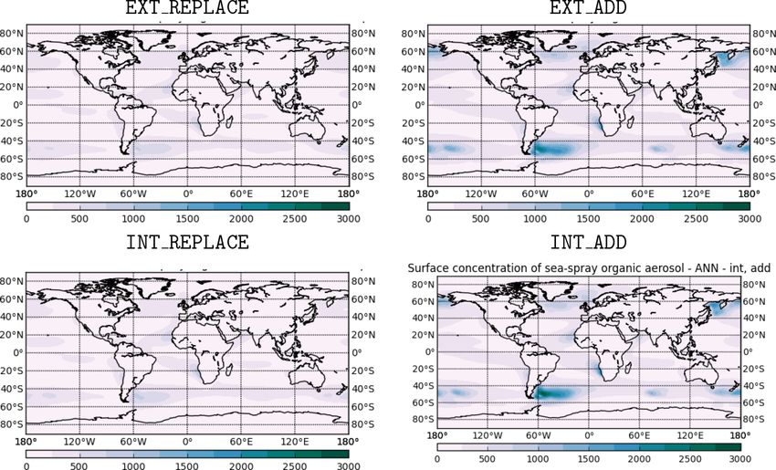
5226                                       S. M. Burrows et al.: OCEANFILMS MOA: implementation and climate sensitivity

is the default aerosol microphysics in CAM5.3. MAM3 rep-           Consequently, we do not extensively evaluate the model’s
resents the aerosol size distribution by means of three log-       aerosols and clouds here. Instead, we focus on the addition
normal modes; MAM4 extends this treatment by adding a              of a source of sea spray aerosol organic matter and its impact
fourth, insoluble submicron aerosol mode (the primary car-         on simulated sea spray aerosol chemistry and clouds.
bon mode), which carries primary organic carbon (POC) and
black carbon (BC) aerosols. This modification significantly        2.2   Introduction of MOA tracers
improves the simulated concentrations of POC and BC rel-
ative to MAM3 simulations, at a lower computational cost           The unmodified MAM4 model carries the following chem-
than a more detailed seven-mode treatment. The impact of           ical species: sea salt, dust, sulfate, SOA, BC, and all non-
MAM4 on simulated aerosol in CAM5.3 is described in Liu            MOA primary organic aerosol (POA), e.g., from terrestrial
et al. (2016).                                                     combustion sources and ship emissions. Each species is char-
   Specific refinements to the MAM aerosol treatments used         acterized by physical properties describing its optical prop-
herein and evaluations of simulated aerosol species with re-       erties, density, and hygroscopicity, summarized in Table 1.
spect to observations have been documented in a series of          POA is also referred to as primary organic matter (POM).
prior publications. Wang et al. (2013) document a number           The chemical species carried in each mode of the MAM4
of improvements to representations of aerosol–cloud interac-       are identified in Table 2. In the model version used here,
tions that improve simulated remote aerosol concentrations         the coarse mode also contains BC, SOA, and POA. Each
in remote regions and the mid to upper troposphere, partic-        mode’s lognormal size distribution is defined by its prog-
ularly for BC aerosol. Simulation of sulfate aerosol is dis-       nostic aerosol number and mass mixing ratios and a fixed
cussed in greater detail in Yang et al. (2017). Biomass burn-      geometric standard deviation (σg ) (Table 2), and the mode’s
ing aerosol is the focus of Das et al. (2017), which compares      number-median diameter (Dgn ) is a diagnostic variable.
CAM5 with several other global models. Aerosol lifetimes              In order to fully represent primary MOA in the model and
are evaluated and compared with 18 other global models in          allow for the specification of chemical properties particular
Kristiansen et al. (2016).                                         to this class of particles, we introduced an additional aerosol
   The simulation of aerosol indirect effects in variants of       chemical species into the model, which we term “MOA”.
CAM5 is documented and discussed in detail in several              MOA tracers were introduced into the model in each of the
previous papers (Ghan et al., 2016; Zhang et al., 2016;            MAM4 aerosol modes.
Gryspeerdt et al., 2017). Ghan et al. (2016) developed a
framework for calculating aerosol indirect effects as the re-      2.3   Sea spray emissions
sult of a chain of contributing response functions and quan-
tify the strength of each term for nine different global models,   Sea spray aerosol in MAM is emitted according to the pa-
including both CAM5.3 and the Pacific Northwest National           rameterization of Mårtensson et al. (2003) for particle diam-
Laboratory (PNNL) configuration of CAM5.3 that includes            eters from 20 nm to 2.5 µm and Monahan (1986) from 2.5
the modifications described above (i.e., MAM4 and modifi-          to 10 µm. The Mårtensson et al. parameterization is based
cations to aerosol–cloud processes). Gryspeerdt et al. (2017)      on laboratory simulations of particle production, using a sin-
document the sensitivity of cloud-top droplet number con-          tered glass filter to generate a bubble plume leading to bub-
centration to various aerosol proxies, such as CCN number          ble bursting and emissions. These experiments used synthetic
(at S = 0.3 % supersaturation) at 1 km, for CAM5.3 and other       seawater, i.e., pure Milli-Q water with the addition of syn-
models.                                                            thetic sea salt. Synthetic sea salt concentrates also contain
   For clarity, we would like to alert readers that the atmo-      trace amounts of dissolved organic carbon (Arnold et al.,
sphere model in the released version of E3SMv1 differs in          2007), although their representativeness for natural seawater
several key respects from the early pre-release version of         is unclear. The Monahan (1986) parameterization, by con-
E3SM used in this study. Notably, in E3SMv1, the cloud pa-         trast, was derived from whitecap simulation experiments in a
rameterization has been replaced with the CLUBB (Cloud             tank filled with natural seawater collected from open coastal
Layers Unified By Binormals) scheme, and the number of             waters.
vertical layers has been increased from 30 layers to 72 layers.
Aerosols, clouds, and aerosol–cloud interactions in E3SMv1         2.4   Emissions of MOA according to OCEANFILMS
have been described and evaluated elsewhere (Xie et al.,
2018; Golaz et al., 2019; Zhang et al., 2019; Wang et al.,         The OCEANFILMS parameterization, introduced and de-
2020).                                                             scribed in detail in Burrows et al. (2014), proposes a mecha-
   In summary, the aerosols and clouds in CAM5.3, the mod-         nistic approach for connecting emissions of MOA to models
ifications that are included here in the EAM, and the im-          of ocean biogeochemistry. As described previously in Bur-
pacts of those modifications on the simulated aerosol and          rows et al. (2014), we used the Parallel Ocean Program (POP;
aerosol–cloud interactions have been documented and dis-           Maltrud et al., 1998) to simulate the ocean’s general circu-
cussed in detail in the previous studies referenced above.         lation and its biogeochemical elemental cycling (BEC) rou-

Atmos. Chem. Phys., 22, 5223–5251, 2022                                             https://doi.org/10.5194/acp-22-5223-2022

S. M. Burrows et al.: OCEANFILMS MOA: implementation and climate sensitivity                                                                                             5227

Table 1. Aerosol species and material properties used in the model simulations.

                                Abbreviation         Name                                 Density (kg m−3 )          Hygroscopicity (κ)
                                MOA                  MOA                                                  1601       0.1
                                NCL                  Sea salt                                             1900       1.16
                                POA                  Primary organic matter                               1000       1.0 × 10⁻¹⁰
                                SOA                  Secondary organic matter                             1000       0.14
                                SO4                  Sulfate aerosol                                      1000       0.507
                                DST                  Dust                                                 2600       0.068
                                BC                   Black carbon                                         1700       1.0 × 10⁻¹⁰

Table 2. MAM4 modes and their size parameters and tracers carried, including number (N) and species mass Mspecies .

                                  Size range                   Nominal        Low bound          High bound          Species
                                                      σg       Dgn (m)          Dgn (m)             Dgn (m)
          Aitken                  20–80 nm            1.6     2.6 × 10⁸        8.70 × 10⁹          5.20 × 10⁸        N , MSO4 , MSOA , MNCL , MMOA
          Accumulation            80 nm–1 µm          1.8     1.1 × 10⁷        5.35 × 10⁸          4.40 × 10⁷        N , MSO4 , MSOA , MPOA , MBC ,
                                                                                                                     MDST , MNCL , MMOA
          Coarse                  1–10 µm             1.8     2.0 × 10⁶        1.00 × 10⁶          4.00 × 10⁶        N , MSO4 a , MSOA a , MPOA a , MBC a ,
                                                                                                                     MDST , MNCL , MMOA
          Primary carbon          80 nm–1 µm          1.6     5.0 × 10⁸        1.00 × 10⁸          1.00 × 10⁷        N, MPOA , MBC , MMOA
        The original formulation of MAM4 did not contain MSO4 MBC , MSOA , and MPOA in the coarse mode (Liu et al., 2016). These species were added to the
        coarse mode as part of the resuspension treatment discussed in this paper, as mass from any species can be transferred to the coarse mode during resuspension.

tines (Moore et al., 2004) to simulate marine biogeochem-                                    While OCEANFILMS predicts the OMF solely as a func-
istry. Both are components of the Community Earth System                                  tion of the prescribed macromolecule fields, the amount of
Model (CESM; Hurrell et al., 2013; UCAR, 2021). Calcula-                                  emitted MOA depends on the combination of the OMF with
tions of the ocean biogeochemistry fields were performed us-                              the emitted sea spray, which is a function of wind speed and
ing the CESM 1.0 beta release 11. Because it uses prescribed                              sea surface temperature. The application of OMF to the sea
input files obtained from simulations performed with the                                  spray emissions requires additional assumptions regarding
earlier POP ocean model rather than online-simulated bio-                                 the mixing state and the impact of organic emissions on total
geochemistry fields, the current implementation of OCEAN-                                 emitted particle number and mass, which we explore in four
FILMS in E3SM is not affected by the large biases in predic-                              sensitivity cases (described in Sect. 3.1).
tion of ocean biogeochemistry that have been documented in
the first release version of E3SM (Burrows et al., 2020).
                                                                                          2.5     Participation of MOA in transport, aerosol and cloud
   Monthly-mean concentrations of five broad classes of
                                                                                                  microphysical processes, and loss processes
macromolecules in ocean surface waters are derived from the
POP-simulated distributions of phytoplankton, zooplankton,                                Aerosol particles evolve through a large number of pro-
and semi-labile dissolved organic carbon and are provided                                 cesses, including transport (by resolved winds, turbulent
to E3SM through prescribed input files. The files containing                              mixing, convective cloud updrafts and downdrafts, gravita-
these macromolecular distributions are publicly available as                              tional sedimentation, or dry deposition), emissions, micro-
part of the E3SM input data repository (see data availability                             physical processes (condensation and evaporation of trace
statement).                                                                               gases, including water vapor, homogeneous nucleation, co-
   Chemical and physical properties are assigned to each of                               agulation, aging), and cloud or precipitation processes (aque-
these macromolecular classes, based on representative proxy                               ous chemistry in cloud droplets, activation, resuspension
molecules for which laboratory measurements are available.                                from evaporating cloud droplets and rain, in-cloud and
Using a Langmuir isotherm-based approach, OCEANFILMS                                      below-cloud wet removal by both stratiform and convective
then predicts the surface coverage of ocean bubble films with                             clouds, or precipitation). MOA participates in almost all of
each of these model macromolecules. This surface film cov-                                these processes within the model.
erage, together with a prescribed bubble film thickness, de-                                 MAM assumes that, within each mode, particles are inter-
termines the OMF of the emitted sea spray aerosol, which is                               nally mixed, so at a given time and location, all particles in a
calculated online within E3SM on the basis of the prescribed                              mode have identical fractional composition (as illustrated in
macromolecule distributions.                                                              Fig. 1). As a result, most processes affect all aerosol species

https://doi.org/10.5194/acp-22-5223-2022                                                                        Atmos. Chem. Phys., 22, 5223–5251, 2022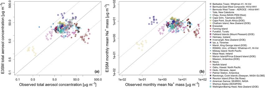
5228                                         S. M. Burrows et al.: OCEANFILMS MOA: implementation and climate sensitivity

                                                                      drop is generally formed from thousands of cloud droplets,
                                                                      and the CCN on which each cloud droplet formed, the re-
                                                                      suspended particle is generally of coarse-mode size (Wang
                                                                      et al., 2020). This differs from the earlier MAM treatment
                                                                      (Liu et al., 2012) in which particles resuspended from evap-
                                                                      orating rain are returned to their original mode. This change
                                                                      mainly affects aerosol number concentrations (the number of
                                                                      particles resuspended is much smaller in the new treatment)
                                                                      and has a minor impact on aerosol mass concentrations.

                                                                      2.6   Optical and cloud-forming properties of MOA
                                                                      Particle CCN activation is determined by the Abdul-Razzak
Figure 1. Illustration of internal versus external mixing states of
                                                                      and Ghan scheme (Abdul-Razzak et al., 1998; Abdul-Razzak
sea spray aerosol upon emission. The emitted aerosol contains both
sea salt (blue) and organic matter (yellow).
                                                                      and Ghan, 2000; Ghan et al., 2011). The prescribed hygro-
                                                                      scopicity for MOA is κMOA = 0.1 (which is the hygroscop-
                                                                      icity of, for example, xanthan gum, sometimes used as a
                                                                      proxy for marine organic matter; Dawson et al., 2016) com-
within a mode in an identical manner. For example, if 5 %             pared with a sea salt hygroscopicity of κNCl = 1.16. The pre-
(on a mass basis) of the Aitken mode particles coagulate with         scribed density of MOA is 1601 kg m−3 (the density of al-
accumulation-mode particles during a model time step, then            ginic acid, a polysaccharide found within algal cell walls)
5 % of the mass of each Aitken mode species is transferred            compared with a sea salt density of 1900 kg m−3 (Table 1).
to the corresponding accumulation-mode species. Thus, ex-             The optical properties of MOA are prescribed to be iden-
tending MAM to treat the new MOA species involved few or              tical to those of sea salt aerosol and are parameterized ac-
no changes to process modules and nearly all process mod-             cording to Ghan and Zaveri (2007). MOA did not contribute
ules automatically treat the new MOA species. The excep-              to ice nucleation in the current model configuration, but re-
tion was emissions, where MOA-specific coding was added.              cent research indicates that marine organic particles can act
Also, many processes utilize physical properties that are av-         as ice nucleating particles (INPs) and may be an important
eraged or summed over all species in a mode (e.g., the total          source of INPs to remote marine regions (Knopf et al., 2011;
mass mixing ratio used in many processes or the dry-volume-           Burrows et al., 2013a; Wilson et al., 2015; DeMott et al.,
weighted hygroscopicity used in activation and water uptake           2016; McCluskey et al., 2019; Zhao et al., 2021). Addition-
processes), and the MOA species contribute to these.                  ally, surfactant effects on aerosol activation (due to alteration
   MOA is initially emitted into either the accumulation or           of surface tension) are not treated, but evidence suggests that
primary carbon mode (depending on initial mixing state as-            the organic matter in marine aerosol is highly surface ac-
sumptions; see below) and the Aitken mode. Aitken-mode                tive (Blanchard, 1963; Barger and Garrett, 1970; Blanchard,
particles and their MOA are transferred to the accumulation           1975; Loglio et al., 1985; Giovannelli et al., 1988; Oppo
mode by growth processes (condensation of H2 SO4 and or-              et al., 1999; Mochida et al., 2002; Tervahattu et al., 2002;
ganic vapors and aqueous sulfate production) and coagula-             Cavalli et al., 2004; Facchini et al., 2008b) and that parti-
tion. The transfer by growth processes is termed renaming,            cle activation rates can be significantly modified for aerosol
wherein particles that grow larger than a size cut of ca. 80 nm       particles that contain salts mixed with substantial amounts of
diameter are transferred. Primary carbon-mode particles and           surfactants (e.g., 70 % or more by mass) (Sorjamaa et al.,
their MOA are also transferred to the accumulation mode               2004; McFiggans et al., 2006), suggesting a possible role
by condensational growth and coagulation. The transfer due            for surface activity of marine organic matter in altering the
to condensation is termed aging, and particles that acquire           water uptake and growth of marine aerosol particles (Abdul-
a specified number of sulfate monolayers or a hygroscopi-             Razzak and Ghan, 2004; Ovadnevaite et al., 2011; Petters and
cally equivalent amount of SOA are transferred (Liu et al.,           Kreidenweis, 2013; Ruehl and Wilson, 2014; Ruehl et al.,
2012, 2016). The aging criterion used was three monolay-              2016; Dawson et al., 2016). It has been suggested that or-
ers, which resulted in an effective aging lifetime of approxi-        ganic matter in submicron sea spray, by suppressing aerosol
mately 2 d. The sensitivity of the model’s aerosol lifetime to        hygroscopic growth, may reduce the climate cooling asso-
the aging criterion is discussed in Liu et al. (2016).                ciated with the scattering of sunlight by sea spray particles
   MOA and other aerosol species are also transferred to the          (direct aerosol effect; Randles et al., 2004).
coarse mode through evaporation of rain. When a rain drop
completely evaporates, the aerosol material it contains (from
in and below cloud scavenging that occurred at higher levels)
is resuspended as a coarse-mode particle. Because each rain-

Atmos. Chem. Phys., 22, 5223–5251, 2022                                                 https://doi.org/10.5194/acp-22-5223-2022
S. M. Burrows et al.: OCEANFILMS MOA: implementation and climate sensitivity                                                  5229

Table 3. Simulation sensitivity cases.                                 Next, we briefly summarize the experimental evidence re-
                                                                    garding both assumptions, the implementation of these dif-
      Short name        Description                                 ferent sensitivity cases within the MAM4 modes, and the rea-
      CNTL              Control experiment; no MOA
                                                                    sons INT_ADD was selected as the default case in E3SM.
      INT_ADD           Internal mixing; MOA adds to sea salt
                        (default model)
      INT_REPLACE       Internal mixing; MOA replaces sea salt      3.1.1   Experimental evidence of sea spray mixing state
      EXT_REPLACE       External mixing; MOA replaces sea salt              response to ocean biology
      EXT_ADD           External mixing; MOA adds to sea salt
                                                                    The chemical mixing state of an aerosol population de-
                                                                    scribes the extent to which individual particles contain mul-
3     Model simulations and analysis methods                        tiple chemical constituents (internal mixing) as compared
                                                                    with particles composed of single chemical components that
Several sensitivity simulations were performed, which were          co-exist in a mixed population (external mixing; see the
identical in their configurations, except for changes in two        schematic representation in Fig. 1). The representation of
model physical assumptions specific to MOA emissions,               mixing state in models can have important impacts on simu-
which are described in Sect. 3.1. All simulations were per-         lation of climate-relevant aerosol properties, including cloud
formed as free-running atmosphere-only climate simulations          condensation and ice-nucleating particle concentrations, and
with year 2000 boundary conditions and fixed sea surface            aerosol optical properties (Riemer et al., 2019). In particular,
temperature. Ocean macromolecular concentrations, which             for sea spray, we simulate a mixture of highly hygroscopic
drive the calculation of OMF in emitted aerosol, are pro-           salts with organic matter that has low hygroscopicity. There-
vided to the model as climatological monthly mean values            fore, the representation of mixing state can be expected to
and are the same in each year of the model simulation and           have important impacts on the simulation of cloud conden-
across all sensitivity cases. The model was allowed to spin up      sation nuclei, and it is important to both consider what is
for a full year in order to allow MOA concentrations (initial-      known about the mixing state of sea spray aerosol and un-
ized at zero throughout the atmosphere) to fully equilibrate in     derstand the extent of the model sensitivity to mixing state
the atmosphere. After the first year, 10 additional years were      assumptions.
simulated, and all further analysis was performed using the             The experimental evidence that sheds the most light on
climatological monthly means of the 10 years.                       the chemical mixing state of sea spray comes from artifi-
                                                                    cial sea spray generation experiments, where sea spray parti-
3.1     Description of the control, default, and sensitivity        cles can be measured immediately after emission, minimiz-
        cases                                                       ing the potential for inclusion of secondary organic mate-
                                                                    rial from condensed gases. Experiments in which sea spray
In implementing the emissions of MOA, decisions must be             aerosol is generated by breaking waves in the presence of in-
made about a number of factors, in particular (1) the mixing        duced phytoplankton blooms provide the most realistic phys-
state of the aerosol, especially with respect to sea salt, with     ical model of the sea spray aerosol production process (Ault
which it is co-emitted, and (2) the impact on the total number      et al., 2013; Collins et al., 2013; Prather et al., 2013). These
and mass of particles emitted. Experiments and observations         experiments, combined with single-particle mass spectrom-
currently do not provide precise constraints on how the mix-        etry and electron microscopy, have shown that the smallest
ing state and amount of emitted particles respond to different      emitted particles (up to about 100 nm in diameter) are pri-
ocean biology and chemistry conditions. Therefore, we con-          marily organic, and marine organic matter is typically mixed
ducted sensitivity experiments with four sets of assumptions        internally with sea salt upon emission for intermediate sizes
that bracket the extremes of possible responses.                    (from about 200 nm to 1 µm in diameter). The vast majority
   An overview of the sensitivity cases tested is shown in Ta-      of the largest particles (greater than 1.5 µm in diameter) are
ble 3. In the control simulation, no MOA is emitted. In the         composed almost entirely of inorganic salts, with inorganic
default treatment and three sensitivity cases, MOA is emit-         salts comprising about 20 % of emitted particles, with diam-
ted using different assumptions in each case. In each case,         eters close to 1 µm. Because the MAM4 accumulation mode
we assume either fully “external” (EXT) or fully “internal”         extends from 80 nm to 1 µm, the majority of particles emitted
(INT) mixing, and we assume that marine organic emissions           in this size range are likely internally mixed, but some ex-
either replace or add to the sea salt emissions that are natively   ternally mixed particles (composed either of purely organic
simulated by the model. Of these four sensitivity cases, the        materials or purely inorganic salts) are also emitted in this
INT_ADD case has been selected as the default for E3SM              size range. Therefore, while the internal mixing assumption
and therefore will be given greater attention in our discus-        is likely more consistent with current experimental evidence,
sion of simulated aerosol and cloud impacts.                        it is also important to understand the impact of this simplify-
                                                                    ing assumption through the mixing state sensitivity cases.

https://doi.org/10.5194/acp-22-5223-2022                                            Atmos. Chem. Phys., 22, 5223–5251, 2022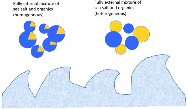
5230                                       S. M. Burrows et al.: OCEANFILMS MOA: implementation and climate sensitivity

3.1.2   Model implementation of sea spray chemical                toplankton exudates, with the magnitude of the increase vary-
        mixing state at emission                                  ing depending on the phytoplankton species from which the
                                                                  exudate was derived.
In MAM4, the chemical species within each aerosol mode               Similarly, Long et al. (2014) also reported an increase in
are treated as internally mixed, an assumption that impacts       aerosol production in the presence of active biological pro-
the calculation of aerosol water uptake, activation, and op-      duction and light and in aerosol generation experiments us-
tical properties. However, MAM4 represents two accumula-          ing a plunging jet system to generate aerosol from natural
tion modes, which are externally mixed from each other: one       seawater, onboard a ship. Increased aerosol production was
of these is termed the “accumulation mode” and contains sol-      observed only during daytime, and only in the biologically
uble aerosol species, while the other is termed the “primary      active waters of George’s Bank (a coastal ecosystem); an in-
carbon mode” and contains insoluble aerosol species. The in-      crease was not observed in the oligotrophic waters of the Sar-
soluble components from the primary carbon mode are even-         gasso Sea. It is unclear, however, what mechanism caused the
tually transferred into the soluble accumulation mode due to      increased aerosol production in these experiments.
aging, which in MAM4 is represented as occurring due to              Finally, field observations have provided mixed evidence
coating by condensation of volatile gases. Sea salt is always     of the impacts of ocean biology on sea spray emission fluxes.
emitted into the soluble accumulation mode. In the “exter-        In several cruises in the North Atlantic, sea spray aerosol was
nally mixed” cases in this study, MOA is emitted into the         produced using a shipboard underway sea spray generator,
primary carbon mode, where it is fully externally mixed with      and campaign-averaged sea spray flux and organic mass frac-
sea salt. In the “internally mixed” cases, MOA is emitted to      tions were reported to show no seasonal differences (Bates
the soluble accumulation mode, together with sea salt. Be-        et al., 2020). In contrast, Sellegri et al. (2021) reported that
cause MAM4 has only one Aitken mode, MOA emissions in             fluxes of sea spray and CCN produced using a similar method
the Aitken mode are internally mixed with all other aerosol       were correlated with concentrations of ocean surface mi-
species in both cases.                                            crobiota (nanophytoplankton cell abundances). Clearly, the
                                                                  source of these apparent discrepancies requires further inves-
3.1.3   Experimental evidence of sea spray number flux            tigation.
        response to ocean biology
                                                                  3.1.4   Model implementation of sea spray number flux
While mixing state is important, a larger impact of ocean bi-             response to MOA
ology on sea spray aerosol could potentially arise if ocean
biology causes shifts in the total number and mass of emit-       To explore the model sensitivity to an assumed increase in
ted particles. However, there are fewer experiments that illu-    sea spray emissions in response to ocean biology, we con-
minate the impacts of ocean biological activity on the total      ducted pairs of sensitivity cases where organic matter is as-
number and mass of particles emitted, and they can be less        sumed to either REPLACE or ADD to the native emissions
straightforward to interpret. Perhaps the clearest experiment     of sea salt aerosol. In REPLACE cases, the mass of emitted
published to date that addresses this question may be from        sea salt is reduced by an amount that is equal to the emit-
Alpert et al. (2015), which reported results from sea spray       ted MOA mass, such that the total emitted aerosol mass re-
aerosol production in a phytoplankton mesocosm experiment         mains constant. The number of emitted sea salt particles is
using a plunging jet system for aerosol generation. They re-      also reduced proportionally in each mode. If the underlying
port an increase in sea spray aerosol particle number concen-     sea spray emission parameterization is assumed to already in-
trations in the tank by a factor of about 3 when phytoplank-      clude the organic content, then the REPLACE option would
ton and bacteria were present in the tank, with the increase      be the more physically plausible approach to implementing
occurring mainly for particles less than 200 nm in diame-         the OMF predicted by OCEANFILMS.
ter. While bubble generation was turned off, particle counts         In contrast, if the underlying sea spray emission parame-
were the same with lights on and off, and the lamps used          terization is assumed to include only the inorganic salt com-
in the experiments put out photosynthetically active radia-       ponents of the emitted spray, then the ADD option would be
tion with wavelengths of 400 to 700 nm (Alpert et al., 2015).     the more physically plausible approach. In the ADD cases,
Thus it is unlikely that the results are due to either SOA for-   the mass and number of emitted sea salt are unchanged from
mation or the more recently recognized mechanism of UV-           the BASE model. Emitted MOA mass is added into the re-
initiated (300–400 nm wavelengths) photosensitized reaction       spective aerosol modes, increasing both the total mass and
pathways at the air–water interface (Rossignol et al., 2016;      the total number of emissions in that mode.
Fu et al., 2015; Tinel et al., 2016; Bernard et al., 2016). A        Note that either the addition of MOA mass (ADD) or the
similar observation was made in an earlier study by Fuentes       replacement of sea salt by MOA (REPLACE) will impact the
et al. (2011), where sea spray aerosol was artificially gener-    volume-weighted hygroscopicity of that mode, which is used
ated by a plunging multi-jet system, and aerosol emissions        in the droplet activation scheme (see Sect. 2.6 and Table 1).
(d < 200 nm) increased substantially in the presence of phy-

Atmos. Chem. Phys., 22, 5223–5251, 2022                                            https://doi.org/10.5194/acp-22-5223-2022
S. M. Burrows et al.: OCEANFILMS MOA: implementation and climate sensitivity                                                5231

3.2    Significance testing                                        winds were arriving from the site’s marine sector; we did
                                                                   not emulate the sectored sampling, but we still include these
The statistical significance of differences induced by the in-     sites in our comparison for consistency with previous studies
troduction of MOA emissions is presented for some key              (e.g., Tsigaridis et al., 2013). The aerosol chemical species
model fields in this paper. In each case, statistical signifi-     measured at these stations typically included sodium, chlo-
cance of changes in a monthly or seasonal mean field was           ride, sulfate, nitrate, and methane sulfonic acid (MSA).
calculated by Welch’s unequal variances t test, treating the          Comparisons between observed and simulated monthly
monthly or seasonal mean from each year of the 10-year sim-        mean climatological aerosol concentrations at the AERO-
ulation as an independent sample. The t statistic was calcu-       CE/SEAREX stations are shown as scatterplots (Fig. 2) for
lated in either each grid box of a 2-D field or at each latitude   both sea salt and total aerosols in the default INT_ADD case.
after zonal averaging of a 2-D field.                              The simulated sea salt burden is typically within a factor of
                                                                   10 of observations. Global model simulations of sea salt ex-
4     Model evaluation with observational data                     hibit considerable diversity (Textor et al., 2006; Gliß et al.,
                                                                   2021), but variations of up to a factor of 10 are typical for
While the overall characteristics of simulated aerosols in this    models of this class (e.g., Tsigaridis et al., 2013). However,
model have been described in detail elsewhere, to provide          we do note that the model falls outside of this range at a few
context for this study, we present a brief observational com-      locations, including the site at Izaña, Tenerife (yellow-filled
parison for simulated sea salt mass, which is particularly rel-    squares), where the model strongly overpredicts observed sea
evant to this study, followed by comparisons of MOA with           salt aerosol concentrations. Sea salt concentrations are un-
available observational datasets. As with any comparison be-       derpredicted at Invercargill, New Zealand, Funafuti, Tuvalu;
tween a global model and in situ observations, the model–          the Bermuda West tower, and sometimes at Miami. At Fu-
observation agreement is limited in part by representative-        nafuti and Bermuda West, where aerosol concentrations are
ness errors and the model’s comparatively coarse resolution;       dominated by sea salt, the model also underpredicts the total
i.e., observations will not always be representative of a model    aerosol by a similar amount.
grid cell. In addition, field campaign data, which are affected
by the weather and wind patterns of a particular time pe-          4.2   Evaluation of modeled MOA concentrations and
riod, are being compared here with climatologies of monthly              organic mass fraction
mean concentrations from the model, which is an imperfect
comparison. Nevertheless, such comparisons are critical to         We evaluate the simulated MOA concentrations and organic
determining whether the model reproduces broad global ge-          mass fractions using field observations of organic aerosol
ographic and seasonal patterns in observed concentrations          mass from station data and from samples collected aboard
over seasonal timescales, which are less susceptible to er-        ship campaigns.
rors associated with the representativeness of short-term field       Few observations are available that are appropriate for
campaign data.                                                     evaluating the simulated MOA at seasonal timescales in a
                                                                   global model. To be useful for such an evaluation, obser-
                                                                   vations must either (1) be obtained under conditions where
4.1    Total and sea salt aerosol concentrations compared          organic aerosol mass is dominated primarily by the marine
       with in situ observations                                   source or (2) be capable of chemically distinguishing the pri-
Relatively few in situ observations are available that are ap-     mary MOA from secondary and non-marine aerosol sources.
propriate for direct evaluation of sea spray aerosol on cli-       Further, the observation should ideally be obtained over a
matological timescales; e.g., data from individual field cam-      sufficiently long period of time to be presumed to be a rep-
paigns may not capture seasonal and interannual variability.       resentative sample and should sample a sufficient portion of
Therefore, to evaluate the overall simulation of sea spray         the seasonal cycle that responses to ocean biology can be
aerosol, we compare, with a benchmark dataset of in situ           observed. Very few datasets are available that meet these cri-
observational data collected by J. Prospero and colleagues         teria. Among the existing datasets, different studies have re-
at the University of Miami during the 1980s and 1990s,             ported different observed variables. In this section, we de-
the AEROCE/SEAREX dataset. This dataset is freely avail-           scribe and discuss the model–observation comparisons for
able from the AEROCOM benchmark data website (https:               three types of observational constraints on the seasonal cy-
//aerocom.met.no/data, last access: 14 March 2022) and in-         cle of sea spray organic matter – total organic carbon (TOC),
cludes filter measurements from a global network of marine         water-insoluble organic carbon (WIOC), and organic mass
stations, mostly located on islands. Most stations were lo-        fraction (OMF) of sea spray.
cated on windward shores or coasts, and filter samples were
typically collected using a high volume sampler at 2 m above
ground level or mounted on a tower 10–20 m above ground
level. At some sites, sampling was conducted only when

https://doi.org/10.5194/acp-22-5223-2022                                          Atmos. Chem. Phys., 22, 5223–5251, 2022
5232 S. M. Burrows et al.: OCEANFILMS MOA: implementation and climate sensitivity
Figure 2. Comparison of monthly means of long-term observations at AEROCE/SEAREX stations with model climatological monthly
means at the nearest grid point. (a) Comparison of total aerosol concentration. (b) Comparison of sodium aerosol mass concentration.
Because Na is well conserved during transport compared to Cl and sea salt ions, sodium content of modeled sea salt aerosol has been
approximated as 30.77 % of modeled sea salt mass.
4.2.1 Comparison of marine OC and OMF seasonal Comparisons with simulated seasonal cycles from all
cycles with site-based measurements under four model configurations are shown in Fig. 3. In the up-
“clean marine” conditions per left panel, we compare the model with observations
from Amsterdam Island. Overall, the model’s annual mean
We focus first on an evaluation of the seasonal cycles of
matches well with observed Amsterdam Island TOC in
observed organic aerosol mass and OMF in the default
the REPLACE configurations (annual mean bias: −3 %,
INT_ADD model and the three sensitivity cases. For this
EXT_REPLACE; 4 %, INT_REPLACE) and is biased high in
evaluation, we focus narrowly on three coastal and island
the ADD configurations (annual mean bias: 39 %, EXT_ADD;
sites, where long-term observations of organic aerosol are
37 %, INT_ADD). However, positive correlations with the
available that have either been screened for “clean marine”
observed seasonal cycle are achieved only in the ADD con-
conditions (Mace Head, Ireland, and Point Reyes, California)
figurations (ρ = 0.55, EXT_ADD; 0.68, INT_ADD), while the
or been collected in a region with minimal anthropogenic
REPLACE configurations have a seasonal cycle that is anti-
influence (Amsterdam Island, Southern Ocean). In order to
correlated with observations (ρ = −0.19, EXT_REPLACE;
make these comparisons as physically meaningful as possi-
−0.47, INT_REPLACE).
ble, in each case we compare only the quantities reported by
The upper right panel of Fig. 3 compares the seasonal cy-
the respective field experiment. At Amsterdam Island, obser-
cle of WIOC at Mace Head, Ireland. Observations at this
vations were available of TOC and WIOC, while Mace Head
site have been filtered for “clean marine” conditions as de-
observations include WIOC and OMF, and Point Reyes ob-
scribed in Rinaldi et al. (2013); we compare them with
servations were available as OMF.
simulated MOA. At Mace Head, the ADD cases clearly
In our evaluation, we assume that, under “clean marine”
match the observed seasonal cycle far better than the RE-
conditions, WIOC is attributable to primary sea spray organic
PLACE cases, with both a lower annual bias in the annual
matter (following Facchini et al., 2008b), and we therefore
mean (−61 %, EXT_REPLACE; −62 %, INT_REPLACE;
compare this variable directly with model-simulated MOA.
−29 %, EXT_ADD; −35 %, INT_ADD) and a higher correla-
We also focus particularly on the OMF as a metric for model
tion (ρ = 0.56, EXT_REPLACE; ρ = 0.67, INT_REPLACE;
evaluation, because this is the variable directly predicted by
ρ = 0.81, EXT_ADD; ρ = 0.77, INT_ADD). Again, the best
OCEANFILMS. While the prediction of TOC or MOA mass
correlation is achieved in the INT_ADD case.
can be influenced by errors in other model processes (e.g.,
The lower panels of Fig. 3 compare the modeled and ob-
sea salt emissions, wet and dry removal rates, and emissions
served OMF at Mace Head (left) and at Point Reyes, Califor-
of other classes of organic aerosol for TOC), the prediction of
nia (right), where observations have also been screened for
OMF is only minimally influenced by model processes other
“clean marine conditions” in a similar fashion to those from
than the OCEANFILMS partitioning of sea spray emissions.
Mace Head. Although the OMF of emissions is fixed, the
Therefore, measurements of OMF at seasonal scales and un-
ADD cases simulate higher OMF in boundary-layer aerosol
der “clean marine” conditions provide the most direct test of
at Mace Head; such a discrepancy can occur if aerosol from
the OCEANFILMS parameterization.
lower-OMF and higher-OMF region mixes, due to the fact
that the increases in total aerosol number and mass are dis-
Atmos. Chem. Phys., 22, 5223–5251, 2022 https://doi.org/10.5194/acp-22-5223-2022S. M. Burrows et al.: OCEANFILMS MOA: implementation and climate sensitivity 5233
Figure 3. Top: observed and simulated seasonal cycle, observed water-insoluble organic carbon (WIOC), and total organic carbon (TOC)
in aerosol versus modeled marine organic carbon (MOC; converted from marine OM using OM : OC = 1.8), at Amsterdam Island (left:
d < 1.0 µm; Sciare et al., 2009) and Mace Head, Ireland (right: d < 1.5 µm; Rinaldi et al., 2013). Note that the Mace Head samples were
selected for “clean marine” conditions as described in Rinaldi et al. (2013) and that pristine conditions typically prevail at Amsterdam Island.
Dashed lines represent the standard deviation of measurements from the same month, where more than one observation was available for
a given month. Bottom: observed and simulated seasonal cycle, organic mass fraction of aerosol as reported under clean marine sampling
conditions. Left: Mace Head, Ireland (d < 1.5 µm; Rinaldi et al., 2013); right: Point Reyes, California (d < 2.5 µm; Gantt et al., 2011).
proportionately higher in the high-OMF regions for ADD 4.2.2 Comparison with observed TOC seasonal cycle at
cases. Once again, the ADD cases agree better with the Mace unscreened sites
Head observations; at Point Reyes, all four configurations of
the model give nearly identical results. Notably, the model For our default INT_ADD case, we performed additional
reproduces the observed difference between a strong sea- comparisons with studies that have reported measurements of
sonal cycle at Mace Head and a weak or nonexistent sea- the seasonal cycles of total organic carbon (TOC) at coastal
sonal cycle at Point Reyes. Gantt and Meskhidze (2013) ac- and island sites but which did not attempt to screen for “clean
counted for this difference by introducing a dependence of marine” conditions. The advantage of these measurements is
the OMF of emitted aerosol on wind speed; however, Fig. 3 that their interpretation requires fewer assumptions, since it
shows that this difference in seasonal behavior at the two lo- does not require us to assume that the “clean marine” screen-
cations is also present in our simulations in spite of the fact ing procedures have adequately removed continental sources
that OCEANFILMS does not assume a dependence of OMF of organic aerosol. However, the lack of screening also re-
on wind speed. quires us to compare with the total organic aerosol simu-
lated by the model, and the comparison therefore becomes
subject to model errors in other simulated organic aerosol
components, including secondary organic aerosol and par-
ticulate organic carbon from burning of fossil fuels and
https://doi.org/10.5194/acp-22-5223-2022 Atmos. Chem. Phys., 22, 5223–5251, 20225234 S. M. Burrows et al.: OCEANFILMS MOA: implementation and climate sensitivity
biomass. Consequently, this measurement provides a strong these data can be used to gain additional insight into the be-
benchmark for MOA sources only at times and locations havior of OCEANFILMS.
where continental sources are very small and errors in their First, we focus on the seasonal cycle of sea spray flux en-
simulation have negligible impact. Such conditions are fre- hancement predicted by OCEANFILMS. Bates et al. (2020)
quent in the Southern Hemisphere remote oceans but infre- reported that campaign-averaged sea spray number flux from
quent throughout most of the Northern Hemisphere (Hamil- NAAMES did not vary across four campaigns conducted
ton et al., 2014). during different seasons. At first glance, this result seems
We compare observed TOC seasonal cycles with the to- to contradict the assumptions and predictions of OCEAN-
tal organic carbon simulated by the model in the default FILMS, which does predict seasonal cycles in these vari-
INT_ADD case from both continental and marine sources. ables in this region. However, a closer examination is needed
Figure 4 shows the seasonal cycle of simulated monthly that accounts for the times and locations when sampling was
mean Aitken- and accumulation-mode organic carbon mass conducted. Intensive scientific sampling in NAAMES oc-
concentration (INT_ADD), subdivided into MOC, continen- curred only during the months of April–May, September, and
tal primary organic carbon (POC), and continental secondary November (Behrenfeld et al., 2019). Figure 6 (left) shows
organic carbon (SOC) mass concentrations compared with the seasonal cycle of sea spray flux enhancement predicted
climatologically averaged observed PM2.5 OC mass plotted by OCEANFILMS (in the default INT_ADD case) at three
as points. The model’s organic aerosol mass has been con- different latitudes in the NAAMES region and indicates the
verted to OC mass using the OM : OC ratios given in the months during which NAAMES measurements of sea spray
figure caption. Note that the model’s PM2.5 also includes a flux were taken. NAAMES unfortunately was not able to
portion of the coarse-mode aerosol, which is not accounted measure sea spray number fluxes during those months when
for in this comparison. The observations used for this com- OCEANFILMS predicts a potentially detectable signal in
parison are from the compilation by Bahadur et al. (2009), as this region, i.e., the months of May through August.
shown in Tsigaridis et al. (2013). Note that both model and Similarly, NAAMES also reported no detectable differ-
observational values represent climatological monthly means ence between campaign-averaged OMF measured across
where possible for the respective dataset. Model–observation four seasons (Bates et al., 2020). However, OCEANFILMS
agreement is greatly improved at sites where MOA domi- predicts almost no change in OMF in this region (Fig. 6,
nates the OA mass: “Amsterdam Island”, “west of Namibia”, right) despite predicting enhanced OMF during June through
“La Reunion Island”, “Bermuda”, “south-west of Australia”, August in the northern portion of the NAAMES study region.
and “New Caledonia”. For most other sites, MOA contributes It is unclear whether weaker signals might have been
only a small fraction of the total OA and has little impact on present in aerosol OMF or flux that were not observable by
the total OA measurements. NAAMES. With N = 7 or fewer filters analyzed for submi-
Figure 5 shows the observed versus modeled monthly cron OMF of generated aerosol per campaign, in the presence
mean organic aerosol mass concentration for the same obser- of high day-to-day variability (Lewis et al., 2021), NAAMES
vations as shown in Fig. 4. Only the mean value is compared likely had sufficient statistical power to distinguish only
for each station and month. Adding MOA improves model– extremely strong seasonal signals. Even the stronger or-
observation agreement, improving the root-mean-squared er- ganic enrichments that OCEANFILMS predicts would have
ror slightly from 1121 to 1090, although the correlation de- occurred at latitudes around 50◦ N during June and July
creases slightly from 0.62 to 0.59. The small magnitude of (months during which NAAMES did not measure OMF or
the improvement in the objective RMSE metric obscures the sea spray flux) and might not be distinguishable from back-
fact that major improvements have been achieved in pris- ground variability with such a small number of samples.
tine locations where organic aerosol mass is small (Fig. 4) In summary, our comparison with NAAMES data indi-
but which therefore also have a small impact on the RMSE. cates that NAAMES did not measure at locations and times
With the inclusion of marine organic carbon, the simulated where OCEANFILMS predicts a strong signal in OMF or sea
OC mass at all points falls within a factor of 10 of the obser- spray flux. Therefore, it appears that the lack of any seasonal
vations (i.e., between the dashed lines). differences in campaign-averaged OMF and sea spray flux
reported by Bates et al. (2020) is nevertheless fully consis-
tent with an OCEANFILMS implementation that does pre-
4.2.3 Comparison with findings from the NAAMES dict seasonal cycles in these variables.
expedition
4.3 Global MOA budgets and annual mean geographic
Another notable recent field experiment, the NAAMES ex- distribution of MOA concentrations in the four
pedition, observed sea spray flux and chemistry for sea spray sensitivity cases
generated shipboard from surface seawater (Bates et al.,
2020). Given the unique marine aerosol observations col- Here we discuss the simulated MOA budgets and concen-
lected by this campaign, it is worthwhile to consider whether trations in the four sensitivity cases. Figure 7 shows the an-
Atmos. Chem. Phys., 22, 5223–5251, 2022 https://doi.org/10.5194/acp-22-5223-2022You can also read