Non-linear Motion Estimation for Video Frame Interpolation using Space-time Convolutions
←
→
Page content transcription
If your browser does not render page correctly, please read the page content below

Non-linear Motion Estimation for Video Frame Interpolation using Space-time
                                                                         Convolutions

                                                                 Saikat Dutta        Arulkumar Subramaniam         Anurag Mittal
                                                                                Indian Institute of Technology Madras
                                                                                             Chennai, India
                                                                            {cs18s016,aruls,amittal}@cse.iitm.ac.in
arXiv:2201.11407v1 [cs.CV] 27 Jan 2022

                                                                 Abstract                                   based applications such as slow-motion video generation
                                                                                                            (e.g., in sports and TV commercials), video compression-
                                             Video frame interpolation aims to synthesize one or mul-       decompression framework [43], generating short videos
                                         tiple frames between two consecutive frames in a video.            from GIF images [48], novel view synthesis [12] and medi-
                                         It has a wide range of applications including slow-motion          cal imaging [27, 55].
                                         video generation, frame-rate up-scaling and developing                 Earlier methods [15, 24, 30, 40, 51] in this domain rely
                                         video codecs. Some older works tackled this problem by as-         on estimating optical flow between interpolated frame to
                                         suming per-pixel linear motion between video frames. How-          source frames (i.e., neighboring frames). Once the opti-
                                         ever, objects often follow a non-linear motion pattern in          cal flow is estimated, the interpolated frame can be syn-
                                         the real domain and some recent methods attempt to model           thesized by a simple warp operation from source images.
                                         per-pixel motion by non-linear models (e.g., quadratic). A         However, estimating an accurate optical flow between video
                                         quadratic model can also be inaccurate, especially in the          frames is a hard problem in itself. Thus, some methods
                                         case of motion discontinuities over time (i.e. sudden jerks)       [29, 38, 39] relied on estimating per-pixel interpolation ker-
                                         and occlusions, where some of the flow information may be          nels to smoothly blend source frames to produce the inter-
                                         invalid or inaccurate.                                             polated frame. Further, some hybrid methods [4, 5] were
                                             In our paper, we propose to approximate the per-pixel          also proposed to integrate optical flow and interpolation ker-
                                         motion using a space-time convolution network that is able         nel based approaches, exhibiting better performance than
                                         to adaptively select the motion model to be used. Specif-          earlier class of methods.
                                         ically, we are able to softly switch between a linear and              Most state-of-the-art interpolation algorithms take two
                                         a quadratic model. Towards this end, we use an end-to-             neighboring frames as input to produce the intermediate
                                         end 3D CNN encoder-decoder architecture over bidirec-              frame. As a result, only a linear motion can be modeled
                                         tional optical flows and occlusion maps to estimate the non-       between the frames either explicitly or implicitly. How-
                                         linear motion model of each pixel. Further, a motion re-           ever, objects often follow complex, non-linear trajecto-
                                         finement module is employed to refine the non-linear mo-           ries. To this end, researchers recently focused on lever-
                                         tion and the interpolated frames are estimated by a simple         aging information from more than two neighboring frames
                                         warping of the neighboring frames with the estimated per-          [7, 8, 26, 50, 53].
                                         pixel motion. Through a set of comprehensive experiments,              3D convolutional neural networks have gained success in
                                         we validate the effectiveness of our model and show that           many important computer vision tasks such as action recog-
                                         our method outperforms state-of-the-art algorithms on four         nition [16, 17, 23, 47], object recognition [31], video object
                                         datasets (Vimeo, DAVIS, HD and GoPro).                             segmentation [18] and biomedical volumetric image seg-
                                                                                                            mentation [10]. However, the application of 3D CNNs in
                                         1. Introduction                                                    VFI task is largely unexplored. Recently, Kalluri et al. [26]
                                                                                                            use a 3D UNet to directly synthesize interpolated frames.
                                            Video frame interpolation (VFI) (also known as Video            However, hallucinating pixel values from scratch can lead
                                         temporal super-resolution) is a significant video enhance-         to blurry results and simply copying pixels from nearby
                                         ment problem which aims to synthesize one or more visu-            frames can produce better results [30].
                                         ally coherent frames between two consecutive frames in a               In this work, we propose a novel frame interpolation
                                         video, i.e., to up-scale the number of video frames. Such          method. First, we compute bi-directional flow and occlu-
                                         an up-scaling method finds its usage in numerous video-            sion maps from four neighboring frames and predict a non-

                                                                                                        1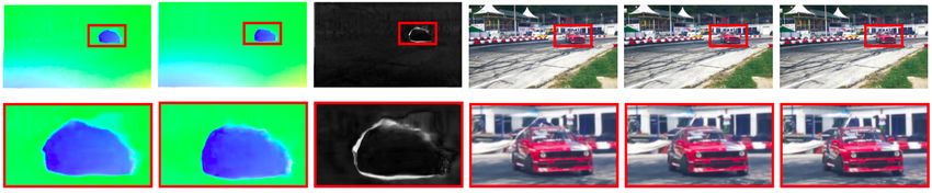
linear flow model with the help of a 3D CNN. In this re-            well. Our work belongs to this category with a key differ-
gard, we formulate a novel 3D CNN architecture namely               ence in that we use a 3D CNN to capture a large spatiotem-
“GridNet-3D” inspired from [52] for efficient multi-scale           poral stride to better estimate per-pixel non-linear motion.
feature aggregation. Further, the predicted non-linear flow         2) Phase-based approaches: Estimating accurate optical
model is used as coefficients in a quadratic formulation of         flow is a hard problem, especially when it involves large
inter-frame motion. The idea is that such an approach can           motion, illumination variations and motion blur. An alterna-
adaptively select between linear and quadratic models by            tive cue to optical flow is to use phase-based modification of
estimating suitable values for the coefficients. Intermedi-         pixels. These methods estimate low-level features such as
ate backward flows are produced through flow reversal and           per-pixel phase [34], fourier decomposition of images using
motion refinement. Finally, two neighboring frames are              steerable pyramids [33], phase and amplitude features us-
warped and combined using a blending mask to synthesize             ing one-dimensional separable Gabor filters [54] to estimate
the interpolated frame. Our algorithm demonstrates state-           the interpolated frame. 3) Kernel-based approaches: Dif-
of-the-art performance over existing approaches on multi-           ferent from optical flow and phase-based methods, kernel-
ple datasets.                                                       based methods strive to estimate per-pixel kernels to blend
   Our main contributions are summarized as follows:                patches from neighborhood frames. Some of these meth-
                                                                    ods employ adaptive convolution [38], adaptive separable
  • We introduce a novel frame interpolation algorithm              convolution [39] or adaptive deformable convolutions [29].
    that utilizes both flow and occlusion maps between
                                                                       Apart from these categories, some methods proposed a
    four input frames to estimate an automatically adapt-
                                                                    hybrid approach to utilize the advantage from multiple cues.
    able pixel-wise non-linear motion model to interpolate
                                                                    For instance, a combination of interpolation kernels and op-
    the frames.
                                                                    tical flow [5] or optical flow and depth [4] are employed to
  • We propose a parameter and runtime-efficient 3D                 obtain complementary features.
    CNN named “GridNet-3D” to aggregate multi-scale
    features efficiently.
                                                                    Multi-frame VFI approaches: Recent methods have
  • Through a set of comprehensive experiments on four              started using multiple frames to capture complex motion
    publicly available datasets (Vimeo, DAVIS, HD and               dynamics between frames. For instance, Choi et al. [8]
    GoPro), we demonstrate that our method achieves                 utilize three frames and bi-directional optical flow between
    state-of-the-art performance.                                   them to generate the intermediate flows and use warping
                                                                    and frame generation module to estimate the final interpo-
   Rest of the paper is organized as follows: Section 2 dis-
                                                                    lated frame. Chi et al. [7] use cubic modeling and a pyramid
cusses some significant prior works in Video Frame Inter-
                                                                    style network to produce seven intermediate frames. Sim-
polation, Section 3 describes our algorithm, Section 4 con-
                                                                    ilarly, Xu et al. [50] use four frames to model a quadratic
tains experiments along with some ablation studies and fi-
                                                                    motion between frames. They estimate quadratic motion
nally Section 5 summarizes limitations of our approach and
                                                                    parameters in terms of an analytical solution involving op-
discusses possible future directions.
                                                                    tical flow. Our method uses four frames and estimates non-
                                                                    linear (quadratic) motion model similar to [50]. However,
2. Related work                                                     we show that using a powerful 3D CNN to estimate the
   In this section, we briefly describe the methods that are        motion parameters instead of an analytical solution signifi-
relevant to this paper.                                             cantly performs better (ref. Section 4.5).

Video-frame interpolation (VFI): Based on the type of
motion cues used, VFI methods can be mainly classified              3D CNN models: 3D CNNs are prevalent in Computer
into three categories: 1) Optical flow based approaches:            Vision tasks involving a spatio-temporal input (video-based
In this class of methods, optical flow [21,32,46] is predomi-       tasks) such as action recognition [16, 17, 23, 47], video ob-
nantly used as a motion cue for interpolating frames. Recent        ject segmentation [18] and video captioning [1, 6]. Related
state-of-the-art methods use fully convolutional networks           to VFI task, Zhang et al. [53] developed a Multi-frame Pyra-
(FCN) [30], 2D UNets [24, 45], multi-scale architectures            mid Refinement (MPR) scheme using 3D UNet to estimate
[44, 51], or bilateral cost volume [40] to predict backward         intermediate flow maps from four input frames. Kalluri et
optical flows to warp the neighboring frames and estimate           al. [26] utilize a 3D encoder-decoder architecture to directly
the interpolated frame. In some methods, forward optical            synthesize interpolated frames from four input frames. Dif-
flow is also utilized [36, 37]. However, these class of meth-       fering from these methods, we use 3D CNN over optical
ods rely on estimating the optical flow based on 2D CNNs            flow and occlusion maps to predict non-linear motion coef-
at the frame-level that might not capture motion features           ficients.

                                                                2
Non-linear                    Backward
                            Motion                         Flow
                           Estimation                    Estimation

                                                                            Motion
                                                                           Refinement

                                                                                         Blending
                                                                                                                 Frame
                                                                                          Mask
                                                                                                                Synthesis
                                                                                        Estimation

Figure 1. Overview of our interpolation algorithm. Non-linear motion estimation module produces forward flow (F0→t , F1→t ), which is
used to generate backward flow (Ft→0 , Ft→1 ). This backward flow is refined using a motion refinement module. Finally, a blending mask
M is estimated that is used to fuse the warped frames to generate interpolated frame It .

                              Flow and
                                                                                                          Quadratic
                              Occlusion                               3D UNet
                              Estimator                                                                  Formulation

                                                                                            Flow
                                                                                        representation

                                          Bidirectional flow and
                                             occlusion masks
Figure 2. Non-linear motion estimation module. First, bi-directional flow and occlusion maps are estimated which are fed to a 3D UNet to
generate flow representation α, β. This flow representation is used to produce forward intermediate flow using quadratic formulation.

3. Space-time convolution network for non-                                       An overview of our framework is shown in Figure 1. The
   linear motion estimation                                                  framework consists of the five modules namely: 1) Non-
                                                                             linear motion estimation (NME) module, 2) Backward flow
    Determining the motion trajectory of pixels is essential                 estimation (BFE) module, 3) Motion refinement (MR) mod-
to determine the transition of pixel values from one frame                   ule, 4) Blending mask estimation (BME) module, and 5)
to the next. Traditional methods use optical flow to achieve                 Frame synthesis. The details of each module are described
this goal with the assumption of brightness constancy and                    in the following sections.
velocity smoothness constraint and use a linear model for
interpolation. While some methods recently have used a                       3.1. Non-linear motion estimation (NME) module
quadratic model for flow estimation with improved results,
such a model is not applicable in certain scenarios such as
motion discontinuities and occlusions. In this work, we opt                     Recent methods attempt to overcome linear motion as-
to use a 3D CNN encoder-decoder architecture to estimate                     sumption by modeling a non-linear motion. Xu et al. [50]
per-pixel non-linear motion that can easily switch between                   proposed to model a quadratic motion model in terms of
a linear and quadratic model. Specifically, the 3D CNN                       time t. i.e., with an assumption that pixel motion follows a
takes a set of bi-directional optical flows and occlusion                    quadratic motion of form αt + βt2 . They estimate the mo-
maps between consecutive video frames {I−1 , I0 , I1 , I2 }                  tion model parameters α, β by an analytical formula derived
to estimate the non-linear motion model that is utilized by                  using per-pixel optical flow. However, such a quadratic as-
other modules to predict an interpolated frame It , where                    sumption cannot be applied to the pixels involving unreli-
t ∈ (0, 1). i.e., the output frame It needs to be coherent in                able optical flow estimates (e.g. occluded pixels). Using
terms of appearance and motion between I0 and I1 .                           such unreliable optical flow estimates may lead to inaccu-

                                                                       3
rate intermediate flow estimation and may end up with er-                 Input

roneous interpolation results. Instead of directly estimating
quadratic motion parameters from optical flow, we attempt
to estimate α, β through a 3D CNN model.
   To learn suitable α and β in the non-linear motion model,
given the input frames {I−1 , I0 , I1 , I2 }, we first estimate bi-
directional flow and occlusion maps between neighboring
frames using a pre-trained PWCNet-Bi-Occ network [19].
Architecture-wise, PWCNet-Bi-Occ is based on state-of-
                                                                                                                     Output    Between   Same
the-art optical flow network PWCNet [46]. It takes two                        Conv 3D    Downsampling   Upsampling
                                                                                                                     conv 3D   stream    stream
                                                                              block      block          block                  path      path
                                                                                                                     layer
frames {Ix , Iy } as input and extracts multi-scale feature
maps of each frame. At each scale, a correlation volume
is computed between corresponding feature maps of the                     Figure 3. Novel GridNet-3D architecture for efficient multi-scale
                                                                          feature aggregation inspired from [52]. It consists of three parallel
frames. Then, bidirectional optical flows {Fx→y , Fy→x }
                                                                          streams operating in different feature resolutions and the commu-
and occlusion maps {Ox→y , Oy→x } are obtained as output                  nication between streams is handled by downsampling and upsam-
at each level by following a coarse-to-fine strategy. We use              pling blocks (refer Sec. 3.1).
the optical flow and occlusion map outputs from the finer
level in our work.                                                        1) to capture spatiotemporal features and 2) to incorpo-
   The           bi-directional             optical          flows        rate multi-scale features efficiently. 3D CNN networks
{Fi→(i+1) , F(i+1)→i }2i=−1       and         occlusion      maps         are the natural choices to capture spatiotemporal features
{Oi→(i+1) , O(i+1)→i }2i=−1 are arranged in temporal order                among video frames. However, the existing architectures
and results in a 5D tensor of size B ×6×#frames×H ×W .                    for pixel-wise tasks (e.g., UNet-3D [26]) adopt a single-
Here B, H, W denote batch size, height and width respec-                  stream Encoder-Decoder style architecture that aggregates
tively, and the 6 channels belong to bi-directional optical               multi-scale features by the process of sequential downsam-
flows and occlusion maps. This tensor is passed through a                 pling and skip-connection which may result in information
3D CNN model to estimate a representation of dimension                    loss [13]. Inspired by the success of GridNet [14, 36] in
B × 4 × 2 × H × W . The temporal dimension of 2                           efficiently incorporating multi-resolution features, we for-
corresponds to t = 0 and t = 1. In each temporal slice, we                mulate a novel 3D version of GridNet namely “GridNet-
predict two coefficient maps α and β, each of 2-dimensions.               3D” by replacing its 2D convolutional filters with 3D con-
We refer these coefficients α, β as the flow representation.              volutional filters. GridNet-3D consists of three parallel
Now the per-pixel non-linear motion F0→t of frame I0                      streams to capture features with different resolutions and
towards the interpolated frame It is given by:                            each stream has five convolutional blocks arranged in a se-
                                                                          quence as shown in Fig. 3. Each convolutional block is
                  F0→t = α0 × t + β0 × t2                      (1)        made up of two conv-3D layers with a residual connection.
                                                                          The three parallel streams have channel dimensions of 16,
   Similarly, F1→t is given by:                                           32 and 64 respectively. The communication between the
                                                                          streams are handled by a set of downsampling and upsam-
           F1→t = α1 × (1 − t) + β1 × (1 − t)2                 (2)        pling blocks. The downsampling block consists of spatial
                                                                          max pooling of stride 2 followed by one conv-3D layer,
   Estimating the coefficients α0 , β0 , α1 and β1 through a              whereas the upsampling block consists of one bilinear up-
neural network instead of an analytical solution [50] of-                 sampling layer followed by two conv-3D layers.
fers the following advantages: 1) The network can flex-                       We perform a set of comparative studies with preva-
ibly choose between linear and non-linear motion. For                     lent architectures such as UNet-3D [26], UNet-2D [24] and
pixels to follow a linear motion, the network may predict                 demonstrate the results in the Sec. 4.4.
β = 0; 2) Unlike [50], learned estimates of α’s, β’s are bet-
ter equipped to handle occlusion by utilizing the occlusion               3.2. Backward flow estimation (BFE) module
maps, 3) Having access to large temporal receptive field
of 4 frames, the non-linear motion coefficients estimated                     The non-linear motions (F0→t , F1→t ) estimated in NME
                                                                          module are forward intermediate flows. To make use of
through a 3D CNN can determine more accurate motion
                                                                          backward warping operation [22] on the frames I0 and
than [50] which rely on optical flow to estimate the coeffi-              I1 , we require the backward intermediate flows (Ft→0 and
cients. Figure 2 shows the pipeline of the non-linear motion              Ft→1 ) to be determined. To achieve this, we use a differen-
estimation module.                                                        tiable flow reversal layer proposed by [50] to obtain Ft→0
   Network specification: We formulate the NME mod-                       and Ft→1 from F0→t and F1→t respectively. Backward
ule to predict α, β with two crucial design choices in mind:              flow at a pixel position x is formulated as weighted average

                                                                      4
of forward flows of all pixels p that fall into neighborhood                  Vimeo Septuplet dataset: Vimeo Septuplet dataset [51] con-
of pixel x. Ft→0 at pixel position x = (x, y) is given by,                sists of 72,436 frame-septuplets of resolution 256 × 448. This
             P                                                            dataset is divided into a training subset of 64,612 septuplets and a
                p+F0→t (p)∈N (x)   w(x, p + F0→t (p))(−F0→t (p))          test subset of 7,824 septuplets. We use 1st , 3rd , 5th and 7th frame
Ft→0 (x) =           P
                        p+F0→t (p+F0→t (p))∈N (x)   w(x, p)               from the septuplets as input frames and predict the 4th frame as
                                                          (3)             interpolation ground truth. We use training subset of this dataset
 where N (x) denotes a 2 × 2 neighborhood around x and w(., .)            for training and evaluate the model on other datasets without fine-
is a weighting function given by:                                         tuning.
                                           2                                  DAVIS dataset: DAVIS-2017 TrainVal dataset [42] contains
                      w(a, b) = e−||a−b||2                      (4)       90 video clips with diverse scenes and complex motions. We uti-
                                                                          lize its 480p counterpart for evaluation purposes. We extract 2,849
   Following similar procedure in Equation 3, Ft→1 is computed
                                                                          quintuplets from the provided video sequences.
from F1→t .
                                                                              HD dataset: Bao et al. [5] collected 11 HD videos consisting
3.3. Motion refinement (MR) module                                        of four 544p, three 720p and four 1080p videos. We extract 456
                                                                          quintuplets from these videos and discard 8 quintuplets with blank
    To further refine the estimated backward flows (Ft→0 and              frames and scene changes. Finally, we use 448 quintuplets for
Ft→1 ), we use a learning based motion refinement approach [50].          evaluation.
To this end, the refinement network takes concatenated source                 GoPro dataset: GoPro dataset proposed by Nah et al. [35]
frames, warped frames and flow maps as input and applies a fully          contains 33 720p videos captured at 720 FPS. We extract 1,500
convolutional network to generate per-pixel offset (∆x, ∆y) and           sets of 25 images from the test split consisting of 11 videos. We
residuals (r(x, y)).                                                      use 1st , 9th , 17th and 25th frames as input frames and 13th frame is
                           r
    Refined optical flow, Ft→0 at pixel (x, y) is given by:               used as the interpolation target.
        r
       Ft→0 (x, y) = Ft→0 (x + ∆x, y + ∆y) + r(x, y)            (5)
                                                                          4.2. Training Details
                                                    r
   Ft→1 is refined in a similar manner to obtain Ft→1 .
                                                                             We develop our models using the Pytorch [41] framework.
   We try with two types of motion refinement network in this
                                                                          During training, we optimize the network using Adam optimizer
work namely: 1) UNet-2D [45,50], and 2) GridNet-2D [11,14,36].
                                                                          [28] with the following hyper-parameters: batch size = 64, β1 =
Finally, we choose GridNet-2D as the motion refinement network
                                                                          0.9 and β2 = 0.999, input frame size = random crop of 256×256.
due to its superior performance (ref. Section 4.6).
                                                                          The learning rate is initially set to 2 × 10⁻⁴ and is divided by a
3.4. Blending mask estimation (BME) module                                factor of 10 when the loss plateaus. The PWCNet-Bi-Occ net-
                                                                          work [19] is fixed until the learning rate reaches the value 2×10⁻⁶
                                       r          r
    The refined backward motions Ft→0      and Ft→1     are used to       and then, it is fine-tuned with the whole network. The model takes
warp images I0 and I1 to yield two estimates It0 , It1 for inter-         around 16 epochs to converge. Code will be released in Github
polated frame It . However, merging these two estimates is not            upon acceptance.
straight-forward. The naive approach of averaging the two esti-
mates and using it as interpolated frame It gives sub-par results.        4.3. Objective Functions
To improve the quality of interpolated frame, we use a learnable
CNN that takes input as the stack of warped frames and intermedi-             Following prior work [24], we use following loss functions to
ate feature maps from previous step to output a soft blending mask        train our model.
M . The BME module consists of three convolutional layers fol-                Reconstruction Loss: We use L1 loss to capture the recon-
lowed by a sigmoid activation function [50] to generate the mask          struction quality of predicted intermediate frames. Reconstruction
M.                                                                        loss Lr is given by,

3.5. Frame synthesis                                                                               Lr = Iˆt − It                            (7)
                                                                                                                     1
    We linearly blend the warped frame using blending mask [24]
                                                                        Here, Iˆt and It refer to the predicted interpolated RGB frame,
computed from the BME module. The final interpolated frame It
                                                                        ground-truth RGB frame respectively.
is given by:
                                                                            Perceptual Loss: Difference between features extracted from
                               r                                  r
      (1 − t) × M     bw(I0 , Ft→0 ) + t × (1 − M )      bw(I1 , Ft→1 ) initial layers of a pre-trained image classification network can help
Iˆt =                                                                   to generate images of higher perceptual quality [25]. Perceptual
                       (1 − t) × M + t × (1 − M )
                                                                (6)     loss Lp is given by:
where bw(., .) denotes the backward warping function.
                                                                                               Lp = φ(Iˆt ) − φ(It )                        (8)
                                                                                                                         2
4. Datasets, Experiments, Results
                                                                              where φ(.) denotes function that generates features from
4.1. Datasets
                                                                          conv4 3 layer of pretrained VGGNet-16.
    We have used the following datasets of different image resolu-            Warping Loss: L1 loss between warped frames and ground
tions in our experiments.                                                 truth intermediate frames is used as warping loss because better

                                                                      5
Table 1. Effect of different CNN architectures used in NME module. Best and second best scores are colred in red and blue respectively.
          CNN used         Vimeo Septuplet        DAVIS              HD                 GoPro           Params Runtime
            in NME         PSNR     SSIM      PSNR      SSIM   PSNR       SSIM     PSNR      SSIM         (M)         (s)
           UNet-2D         34.76   0.9537     27.34     0.8254 31.21     0.8971    28.90     0.8793      38.30       0.18
           UNet-3D         34.96   0.9545     27.46     0.8278 31.31     0.8976    29.01     0.8826      60.55       0.37
          GridNet-3D       34.99   0.9544     27.53     0.8281 31.49     0.9000    29.08     0.8826      20.92       0.32

                               Input images       UNet-2D             UNet-3D              GridNet-3D       Ground Truth

                        Figure 4. Qualitative comparison between different CNN architectures used in NME module.

                               Table 2. Quantitative comparison between UNet and GridNet as MR module.
      Motion Refinement        Vimeo Septuplet         DAVIS               HD               GoPro                          Params   Runtime
           module              PSNR     SSIM       PSNR     SSIM     PSNR     SSIM     PSNR     SSIM                         (M)      (s)
          UNet-2D              34.70    0.9532     27.32    0.8260   31.02    0.8944   28.81   0.8798                       78.11    0.37
        GridNet-2D             34.96    0.9475     27.46    0.8278   31.31    0.8976   29.01   0.8826                       60.55    0.37

                             Input Images              UNet-2D as                 GridNet-2D as             Ground Truth
                                                       MR module                   MR module
                                        Figure 5. Qualitative comparison between different MR modules.

flow predictions mean warped frames will be closer to ground truth              4.4. Experiments on model configurations
intermediate frame.
                                                                                    In this section, we perform comparative studies among the dif-
                                                                                ferent choices available for NME (UNet-2D [24], UNet-3D [26],
                       r                        r
   Lw = kIt − bw(I0 , Ft→0 )k1 + kIt − bw(I1 , Ft→1 )k1             (9)         GridNet-3D) and MR (UNet-2D [45], GridNet-2D [14]) modules
                                                                                to determine the best performing configuration.
    Here bw(.,.) denotes the backward warping function.
    Smoothness Loss: Total variation (TV) loss is used as smooth-                   Choice of NME module: We experiment with three differ-
ness loss to ensure smoothness in intermediate optical flow predic-             ent architectures for NME module: 1) UNet-2D [24], 2) UNet-
tion.                                                                           3D [26], and 3) novel GridNet-3D proposed in this paper. We il-
                             r             r                                    lustrate the quantitative performance with different NME modules
                  Ls = k∇Ft→0   k1 + k∇Ft→1    k1              (10)
                                                                                in Table 1 along with number of parameters and runtimes. We
   Our final loss is a linear combination of all the loss functions
                                                                                observe that 3D-CNN version of NME modules perform superior
described above.
                                                                                to UNet-2D in general. Further, GridNet-3D performs better than
               L = λr Lr + λp Lp + λw Lw + λs Ls                 (11)           UNet-3D in DAVIS, HD and GoPro datasets while having less pa-
                                                                                rameters and runtime.
We choose λr = 204, λp = 0.005, λw = 102 and λs = 1
                                                                                    Choice of MR modules: We experiment with two types of
similar to unofficial SuperSloMo repository [3]. When the model
                                                                                motion refinement modules: UNet-2D [45] and GridNet-2D [14].
is trained with low learning rate at later phase, we turn off warping
                                                                                We use a standard encoder-decoder architecture with skip connec-
loss and smoothness loss by setting λw and λs to 0. This helps
                                                                                tions for UNet-2D. In GridNet-2D, encoder and decoder blocks are
network to focus on improving the final reconstruction quality of
                                                                                laid out in a grid-like fashion to carry through multi-scale feature
interpolated frame.
                                                                                maps till the final layer. Quantitative comparison in Table 2 shows
   1 BMBC   encountered out-of-memory error when tested on HD dataset.          that using GridNet-2D as MR module performs significantly bet-

                                                                          6
Table 3. Quantitative comparison with state-of-the-art methods. Best and second best scores are colred in red and blue respectively. * -
TOFlow [51] was trained on Vimeo-Triplet dataset, all other methods are trained in Vimeo-Septuplet dataset.

                          Input     Vimeo Septuplet          DAVIS                    HD                GoPro           Params     Runtime
        Method
                         frames     PSNR    SSIM         PSNR    SSIM         PSNR      SSIM       PSNR     SSIM          (M)         (s)
    TOFlow* [51]            2       33.46   0.9399       25.49  0.7577        30.94     0.8854     27.08   0.8286         1.07       0.10
    SepConv [39]            2       33.04   0.9334       25.38  0.7428        30.24     0.8784     26.88   0.8166         21.6      0.024
   SuperSloMo [24]          2       33.46   0.9423       25.84  0.7765        30.37     0.8834     27.31   0.8367        39.61      0.025
       CAIN [9]             2       31.70   0.9106       24.89  0.7235        29.22     0.8523     26.81   0.8076        42.78       0.02
     BMBC1 [40]             2       31.34   0.9054       23.50  0.6697          -          -       24.62   0.7399         11.0       0.41
   Tridirectional [8]       3       32.73   0.9331       25.24  0.7476        29.84     0.8692     26.80   0.8180        10.40       0.19
       QVI [50]             4       34.50   0.9521       27.36  0.8298        30.92     0.8971     28.80   0.8781        29.22       0.10
     FLAVR [26]             4       33.56   0.9372       25.74  0.7589        29.96     0.8758     27.76   0.8436        42.06       0.20
         Ours               4       34.99   0.9544       27.53  0.8281        31.49     0.9000     29.08   0.8826        20.92       0.32

                Input Images      SuperSloMo          QVI        Tridirectional       FLAVR           Ours       Ground Truth
                           Figure 6. Qualitative comparison of our method with other state-of-the-art algorithms.

ter than UNet-2D. Qualitative comparison in Figure 5 illustrates               Our method achieves best PSNR and SSIM scores in Vimeo,
that GridNet-2D reduces the smudge effect in interpolated frame             HD and GoPro datasets. Our method performs best in PSNR and
compared to UNet-2D. From Table 2, we can also infer that using             second best in SSIM metric on DAVIS dataset. Qualitative com-
GridNet-2D as MR module reduces total number of parameters of               parison with other methods is shown in Figure 6.
the model while the runtime remains constant.
    Based on these experiments, we use GridNet-3D in NME mod-               4.6. Ablation studies
ule and GridNet-2D as MR module in state-of-the-art comparisons                 Choice of input features (RGB vs. Flow+Occlusion): To
and in ablation studies unless specified otherwise.                         demonstrate the importance of flow and occlusion maps, we per-
                                                                            form an experiment where we use RGB frames as input to the
4.5. Comparison with state-of-the-arts
                                                                            3D CNN. Quantitative comparison between these two approaches
    We compare our model with multiple state-of-the-art meth-               are shown in Table 4 with number of parameters and runtimes.
ods: TOFlow [51], Sepconv-L1 [39], SuperSloMo [24], CAIN [9],               Both experiments in Table 4 use UNet-2D as MR module. We
BMBC [40], QVI [50], Tridirectional [8] and FLAVR [26]. For                 observe that Flow+Occlusion maps as input performs better than
comparison with TOFlow, official pretrained model [2] is used.              RGB frames. Qualitative comparison in Figure 7 shows that in-
For all other models, we train them on Vimeo-Septuplet train set            terpolated results are more accurate when Flow+Occlusion maps
with same learning rate schedule and batch size as ours for fair            are used compared to RGB. Note that, our model with RGB in-
comparison. We use unofficial repositories of SuperSloMo [3]                put already performs better than FLAVR [26] (refer to Table 3).
and Sepconv [20] to train the corresponding models. Please note,            This signifies that frame generation by hallucinating pixels from
official pretrained models of other methods might produce differ-           scratch [26] is hard for neural networks to achieve than frame gen-
ent results due to difference in training data and training settings.       eration by warping neighborhood frames.
During evaluation, Peak Signal-to-Noise ratio (PSNR) and Struc-                 Importance of BFE, MR and BME modules: To understand
tural Similarity (SSIM) [49] are used as evaluation metric to com-          the importance of BFE, MR and BME modules, we re-purpose the
pare performances. Quantitative comparisons with state-of-the-art           NME module to directly predict non-linear backward flows Ft→0 ,
methods on Vimeo, DAVIS, HD and GoPro datasets are shown in                 Ft→1 and blending mask M . In this experiment, we use RGB
Table 3. Number of parameters and average runtime to produce a              frames as input to NME module. The quantitative comparison in
frame of resolution 256 × 448 on NVIDIA 1080Ti GPU for each                 Table 5 illustrates that the direct estimation of backward flows,
model is also reported.                                                     mask (without BFE, MR and BME) performs sub-par to estimat-

                                                                        7
Table 4. Effect of different input features to 3D CNN.
                             Vimeo Septuplet        DAVIS                   HD                GoPro                      Params    Runtime
             Input
                             PSNR    SSIM      PSNR       SSIM       PSNR       SSIM     PSNR     SSIM                     (M)       (s)
            RGB              34.12   0.9474    26.34     0.7883       30.80    0.8854     28.34  0.8642                   61.89     0.23
       Flow + Occlusion      34.70   0.9532    27.32     0.8260       31.02    0.8944     28.81  0.8798                   78.11     0.37

                        Figure 7. Qualitative comparison between RGB and Flow+Occlusion as input to 3D CNN.

                                    Table 5. Quantitative significance of BFE, MR and BME modules.
                                   Vimeo Septuplet          DAVIS                 HD           GoPro                          Params   Runtime
                                   PSNR      SSIM      PSNR       SSIM     PSNR      SSIM  PSNR    SSIM                         (M)      (s)
  without BFE, MR and BME          33.91    0.9443     26.05      0.7686    30.72   0.8811 28.12   0.8583                      42.07    0.20
   with BFE, MR and BME            34.12    0.9474     26.34      0.7883    30.80   0.8854 28.34   0.8642                      61.89    0.23

                              Input frames            Without BFE, MR and BME   With BFE, MR and BME     Ground Truth
Figure 8. Qualitative comparison between intermediate flowmap and blending mask estimation with and without BFE, MR and BME
modules.

                          (QVI)              (Ours)          Flow difference           QVI             Ours             Ground Truth
                                  Figure 9. Intermediate flow visualization between QVI and our approach.

ing them with BFE, MR (UNet-2D) and BME modules. Added                          between neighboring frames are passed as input to a 3D CNN
to this, qualitative comparisons in Figure 8 shows that the direct              to predict per-pixel non-linear motion. This makes our network
estimation of backward flows may lead to ghosting artifacts due to              flexible to choose between linear and quadratic motion models in-
inaccurate flow estimation near motion boundaries.                              stead of a fixed motion model as used in prior work. Our method
    Intermediate flow visualizations: We visualize the backward                 achieves state-of-the-art results in multiple datasets. Since flow
        r
flow Ft→0   estimated by QVI [50] and our approach in Figure 9.                 and occlusion estimates from PWCNet-Bi-Occ are often not accu-
We notice that erroneous results in QVI’s [50] interpolated frame               rate and hence can create a performance bottleneck in interpola-
is caused by incorrect estimation of the backward flow. However,                tion task, further research can explore whether inclusion of RGB
our method remedies this by accurately estimating the backward                  frames as input to 3D CNN can improve the performance. Finally,
flow as visualized in the absolute flow difference map in Figure 9.             flow representation estimation for cubic modeling can also be in-
                                                                                vestigated in future.
5. Conclusion
    In this paper, we presented a 3D CNN based frame interpola-
tion algorithm in which the bi-directional flow and occlusion maps

                                                                            8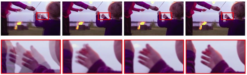
References                                                              [14] Damien Fourure, Rémi Emonet, Élisa Fromont, Damien
                                                                             Muselet, Alain Trémeau, and Christian Wolf. Residual
 [1] Nayyer Aafaq, Naveed Akhtar, Wei Liu, Syed Zulqarnain                   conv-deconv grid network for semantic segmentation. arXiv
     Gilani, and Ajmal Mian. Spatio-temporal dynamics and se-                preprint arXiv:1707.07958, 2017. 4, 5, 6
     mantic attribute enriched visual encoding for video caption-
                                                                        [15] Shurui Gui, Chaoyue Wang, Qihua Chen, and Dacheng Tao.
     ing. In Proceedings of the IEEE/CVF Conference on Com-
                                                                             Featureflow: Robust video interpolation via structure-to-
     puter Vision and Pattern Recognition, pages 12487–12496,
                                                                             texture generation. In The IEEE/CVF Conference on Com-
     2019. 2
                                                                             puter Vision and Pattern Recognition (CVPR), June 2020. 1
 [2] anchen1011.       toflow.    https : / / github . com /
                                                                        [16] Kensho Hara, Hirokatsu Kataoka, and Yutaka Satoh. Learn-
     anchen1011/toflow. 7
                                                                             ing spatio-temporal features with 3d residual networks for
 [3] avinashpaliwal. Super-SloMo. https://github.com/
                                                                             action recognition. In Proceedings of the IEEE International
     avinashpaliwal/Super-SloMo. 6, 7
                                                                             Conference on Computer Vision Workshops, pages 3154–
 [4] Wenbo Bao, Wei-Sheng Lai, Chao Ma, Xiaoyun Zhang,                       3160, 2017. 1, 2
     Zhiyong Gao, and Ming-Hsuan Yang. Depth-aware video
                                                                        [17] Kensho Hara, Hirokatsu Kataoka, and Yutaka Satoh. Can
     frame interpolation. In Proceedings of the IEEE Conference
                                                                             spatiotemporal 3d cnns retrace the history of 2d cnns and im-
     on Computer Vision and Pattern Recognition, pages 3703–
                                                                             agenet? In Proceedings of the IEEE conference on Computer
     3712, 2019. 1, 2
                                                                             Vision and Pattern Recognition, pages 6546–6555, 2018. 1,
 [5] Wenbo Bao, Wei-Sheng Lai, Xiaoyun Zhang, Zhiyong Gao,
                                                                             2
     and Ming-Hsuan Yang. Memc-net: Motion estimation and
                                                                        [18] Rui Hou, Chen Chen, Rahul Sukthankar, and Mubarak Shah.
     motion compensation driven neural network for video inter-
                                                                             An efficient 3d cnn for action/object segmentation in video.
     polation and enhancement. IEEE Transactions on Pattern
                                                                             arXiv preprint arXiv:1907.08895, 2019. 1, 2
     Analysis and Machine Intelligence, 2019. 1, 2, 5
                                                                        [19] Junhwa Hur and Stefan Roth. Iterative residual refinement
 [6] Jingwen Chen, Yingwei Pan, Yehao Li, Ting Yao, Hongyang
                                                                             for joint optical flow and occlusion estimation. In Proceed-
     Chao, and Tao Mei. Temporal deformable convolutional
                                                                             ings of the IEEE/CVF Conference on Computer Vision and
     encoder-decoder networks for video captioning. In Proceed-
                                                                             Pattern Recognition, pages 5754–5763, 2019. 4, 5
     ings of the AAAI Conference on Artificial Intelligence, vol-
     ume 33, pages 8167–8174, 2019. 2                                   [20] HyeongminLEE. pytorch-sepconv. https://github.
 [7] Zhixiang Chi, Rasoul Mohammadi Nasiri, Zheng Liu, Juwei                 com/HyeongminLEE/pytorch-sepconv. 7
     Lu, Jin Tang, and Konstantinos N Plataniotis. All at once:         [21] Eddy Ilg, Nikolaus Mayer, Tonmoy Saikia, Margret Keuper,
     Temporally adaptive multi-frame interpolation with ad-                  Alexey Dosovitskiy, and Thomas Brox. Flownet 2.0: Evolu-
     vanced motion modeling. arXiv preprint arXiv:2007.11762,                tion of optical flow estimation with deep networks. In Pro-
     2020. 1, 2                                                              ceedings of the IEEE conference on computer vision and pat-
 [8] Jinsoo Choi, Jaesik Park, and In So Kweon. High-quality                 tern recognition, pages 2462–2470, 2017. 2
     Frame Interpolation via Tridirectional Inference. Winter           [22] Max Jaderberg, Karen Simonyan, Andrew Zisserman, and
     Conference on Applications of Computer Vision (WACV),                   Koray Kavukcuoglu. Spatial transformer networks. In Pro-
     2021. 1, 2, 7                                                           ceedings of the 28th International Conference on Neural In-
 [9] Myungsub Choi, Heewon Kim, Bohyung Han, Ning Xu, and                    formation Processing Systems-Volume 2, pages 2017–2025,
     Kyoung Mu Lee. Channel attention is all you need for video              2015. 4
     frame interpolation. In AAAI, 2020. 7                              [23] Shuiwang Ji, Wei Xu, Ming Yang, and Kai Yu. 3d convolu-
[10] Özgün Çiçek, Ahmed Abdulkadir, Soeren S Lienkamp,                   tional neural networks for human action recognition. IEEE
     Thomas Brox, and Olaf Ronneberger. 3d u-net: learning                   transactions on pattern analysis and machine intelligence,
     dense volumetric segmentation from sparse annotation. In                35(1):221–231, 2012. 1, 2
     International conference on medical image computing and            [24] Huaizu Jiang, Deqing Sun, Varun Jampani, Ming-Hsuan
     computer-assisted intervention, pages 424–432. Springer,                Yang, Erik Learned-Miller, and Jan Kautz. Super slomo:
     2016. 1                                                                 High quality estimation of multiple intermediate frames for
[11] Saikat Dutta, Nisarg A Shah, and Anurag Mittal. Efficient               video interpolation. In Proceedings of the IEEE Conference
     space-time video super resolution using low-resolution flow             on Computer Vision and Pattern Recognition, pages 9000–
     and mask upsampling. arXiv preprint arXiv:2104.05778,                   9008, 2018. 1, 2, 4, 5, 6, 7
     2021. 5                                                            [25] Justin Johnson, Alexandre Alahi, and Li Fei-Fei. Perceptual
[12] John Flynn, Ivan Neulander, James Philbin, and Noah                     losses for real-time style transfer and super-resolution. In
     Snavely. Deepstereo: Learning to predict new views from the             European conference on computer vision, pages 694–711.
     world’s imagery. In Proceedings of the IEEE conference on               Springer, 2016. 5
     computer vision and pattern recognition, pages 5515–5524,          [26] Tarun Kalluri, Deepak Pathak, Manmohan Chandraker, and
     2016. 1                                                                 Du Tran. Flavr: Flow-agnostic video representations for fast
[13] Damien Fourure, Rémi Emonet, Elisa Fromont, Damien                     frame interpolation. arXiv preprint arXiv:2012.08512, 2020.
     Muselet, Alain Tremeau, and Christian Wolf. Residual                    1, 2, 4, 6, 7
     conv-deconv grid network for semantic segmentation. arXiv          [27] Alexandros Karargyris and Nikolaos Bourbakis. Three-
     preprint arXiv:1707.07958, 2017. 4                                      dimensional reconstruction of the digestive wall in capsule

                                                                    9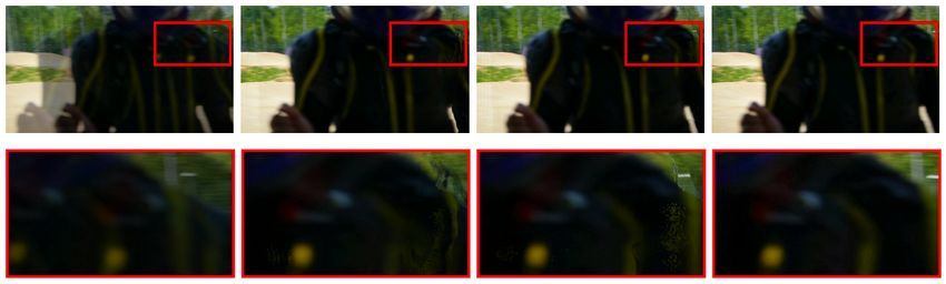
endoscopy videos using elastic video interpolation. IEEE                    Science and Business Media Deutschland GmbH, 2020. 1,
       transactions on Medical Imaging, 30(4):957–971, 2010. 1                     2, 7
[28]   Diederik P Kingma and Jimmy Ba. Adam: A method for                   [41]   Adam Paszke, Sam Gross, Francisco Massa, Adam Lerer,
       stochastic optimization. arXiv preprint arXiv:1412.6980,                    James Bradbury, Gregory Chanan, Trevor Killeen, Zeming
       2014. 5                                                                     Lin, Natalia Gimelshein, Luca Antiga, Alban Desmaison,
[29]   Hyeongmin Lee, Taeoh Kim, Tae-young Chung, Daehyun                          Andreas Kopf, Edward Yang, Zachary DeVito, Martin Rai-
       Pak, Yuseok Ban, and Sangyoun Lee. Adacof: adaptive col-                    son, Alykhan Tejani, Sasank Chilamkurthy, Benoit Steiner,
       laboration of flows for video frame interpolation. In Pro-                  Lu Fang, Junjie Bai, and Soumith Chintala. Pytorch: An im-
       ceedings of the IEEE/CVF Conference on Computer Vision                      perative style, high-performance deep learning library. In H.
       and Pattern Recognition, pages 5316–5325, 2020. 1, 2                        Wallach, H. Larochelle, A. Beygelzimer, F. d'Alché-Buc, E.
[30]   Ziwei Liu, Raymond A Yeh, Xiaoou Tang, Yiming Liu, and                      Fox, and R. Garnett, editors, Advances in Neural Informa-
       Aseem Agarwala. Video frame synthesis using deep voxel                      tion Processing Systems 32, pages 8024–8035. Curran Asso-
       flow. In Proceedings of the IEEE International Conference                   ciates, Inc., 2019. 5
       on Computer Vision, pages 4463–4471, 2017. 1, 2                      [42]   Jordi Pont-Tuset, Federico Perazzi, Sergi Caelles, Pablo Ar-
[31]   Daniel Maturana and Sebastian Scherer. Voxnet: A 3d con-                    beláez, Alex Sorkine-Hornung, and Luc Van Gool. The 2017
       volutional neural network for real-time object recognition.                 davis challenge on video object segmentation. arXiv preprint
       In 2015 IEEE/RSJ International Conference on Intelligent                    arXiv:1704.00675, 2017. 5
       Robots and Systems (IROS), pages 922–928. IEEE, 2015. 1              [43]   Reza Pourreza and Taco S Cohen.              Extending neu-
[32]   Simon Meister, Junhwa Hur, and Stefan Roth. Unflow: Un-                     ral p-frame codecs for b-frame coding. arXiv preprint
       supervised learning of optical flow with a bidirectional cen-               arXiv:2104.00531, 2021. 1
       sus loss. In Proceedings of the AAAI Conference on Artificial        [44]   Anurag Ranjan and Michael J Black. Optical flow estima-
       Intelligence, volume 32, 2018. 2                                            tion using a spatial pyramid network. In Proceedings of the
[33]   Simone Meyer, Abdelaziz Djelouah, Brian McWilliams,                         IEEE conference on computer vision and pattern recogni-
       Alexander Sorkine-Hornung, Markus Gross, and Christo-                       tion, pages 4161–4170, 2017. 2
       pher Schroers. Phasenet for video frame interpolation. In            [45]   Olaf Ronneberger, Philipp Fischer, and Thomas Brox. U-
       Proceedings of the IEEE Conference on Computer Vision                       net: Convolutional networks for biomedical image segmen-
       and Pattern Recognition, pages 498–507, 2018. 2                             tation. In International Conference on Medical image com-
[34]   Simone Meyer, Oliver Wang, Henning Zimmer, Max Grosse,                      puting and computer-assisted intervention, pages 234–241.
       and Alexander Sorkine-Hornung. Phase-based frame inter-                     Springer, 2015. 2, 5, 6
       polation for video. In Proceedings of the IEEE conference on         [46]   Deqing Sun, Xiaodong Yang, Ming-Yu Liu, and Jan Kautz.
       computer vision and pattern recognition, pages 1410–1418,                   Pwc-net: Cnns for optical flow using pyramid, warping,
       2015. 2                                                                     and cost volume. In Proceedings of the IEEE Conference
[35]   Seungjun Nah, Tae Hyun Kim, and Kyoung Mu Lee. Deep                         on Computer Vision and Pattern Recognition, pages 8934–
       multi-scale convolutional neural network for dynamic scene                  8943, 2018. 2, 4
       deblurring. In Proceedings of the IEEE conference on                 [47]   Du Tran, Heng Wang, Lorenzo Torresani, Jamie Ray, Yann
       computer vision and pattern recognition, pages 3883–3891,                   LeCun, and Manohar Paluri. A closer look at spatiotemporal
       2017. 5                                                                     convolutions for action recognition. In Proceedings of the
[36]   Simon Niklaus and Feng Liu. Context-aware synthesis for                     IEEE conference on Computer Vision and Pattern Recogni-
       video frame interpolation. In Proceedings of the IEEE Con-                  tion, pages 6450–6459, 2018. 1, 2
       ference on Computer Vision and Pattern Recognition, pages            [48]   Yang Wang, Haibin Huang, Chuan Wang, Tong He, Jue
       1701–1710, 2018. 2, 4, 5                                                    Wang, and Minh Hoai. Gif2video: Color dequantization and
[37]   Simon Niklaus and Feng Liu. Softmax splatting for video                     temporal interpolation of gif images. In Proceedings of the
       frame interpolation. In Proceedings of the IEEE/CVF Con-                    IEEE Conference on Computer Vision and Pattern Recogni-
       ference on Computer Vision and Pattern Recognition, pages                   tion, pages 1419–1428, 2019. 1
       5437–5446, 2020. 2                                                   [49]   Zhou Wang, Alan C Bovik, Hamid R Sheikh, and Eero P Si-
[38]   Simon Niklaus, Long Mai, and Feng Liu. Video frame in-                      moncelli. Image quality assessment: from error visibility to
       terpolation via adaptive convolution. In Proceedings of the                 structural similarity. IEEE transactions on image processing,
       IEEE Conference on Computer Vision and Pattern Recogni-                     13(4):600–612, 2004. 7
       tion, pages 670–679, 2017. 1, 2                                      [50]   Xiangyu Xu, Li Siyao, Wenxiu Sun, Qian Yin, and Ming-
[39]   Simon Niklaus, Long Mai, and Feng Liu. Video frame inter-                   Hsuan Yang. Quadratic video interpolation. arXiv preprint
       polation via adaptive separable convolution. In Proceedings                 arXiv:1911.00627, 2019. 1, 2, 3, 4, 5, 7, 8, 12
       of the IEEE International Conference on Computer Vision,             [51]   Tianfan Xue, Baian Chen, Jiajun Wu, Donglai Wei, and
       pages 261–270, 2017. 1, 2, 7                                                William T Freeman.          Video enhancement with task-
[40]   Junheum Park, Keunsoo Ko, Chul Lee, and Chang Su Kim.                       oriented flow. International Journal of Computer Vision,
       Bmbc: Bilateral motion estimation with bilateral cost vol-                  127(8):1106–1125, 2019. 1, 2, 5, 7
       ume for video interpolation. In 16th European Conference             [52]   YUE Yuanchen, CAI Yunfei, and WANG Dongsheng.
       on Computer Vision, ECCV 2020, pages 109–125. Springer                      Gridnet-3d: A novel real-time 3d object detection algo-

                                                                       10
rithm based on point cloud. Chinese Journal of Electronics,
30(5):931–939, 2021. 2, 4
[53] Haoxian Zhang, Ronggang Wang, and Yang Zhao. Multi-
frame pyramid refinement network for video frame interpo-
lation. IEEE Access, 7:130610–130621, 2019. 1, 2
[54] Lunan Zhou, Yaowu Chen, Xiang Tian, and Rongxin Jiang.
Frame interpolation using phase and amplitude feature pyra-
mids. In 2019 IEEE International Conference on Image Pro-
cessing (ICIP), pages 4190–4194. IEEE, 2019. 2
[55] Svitlana Zinger, Daniel Ruijters, Luat Do, and Peter HN de
With. View interpolation for medical images on autostereo-
scopic displays. IEEE Transactions on Circuits and Systems
for Video Technology, 22(1):128–137, 2011. 1
116. Appendix
6.1. Importance of using four frames
In order to show the effectiveness of using four frames in our network, we report results of our model using only two frames (I0 , I1 ) as
input. Since our model expects four frames as input, we use frame repetition (I0 , I0 , I1 , I1 ) in this experiment. Quantitative comparison in
Table-6 shows that our model indeed benefits from using four frames as input.
Table 6. Quantitative comparison between using two frames and four frames
No. of Vimeo Septuplet DAVIS HD GoPro
input frames PSNR SSIM PSNR SSIM PSNR SSIM PSNR SSIM
2 33.61 0.9438 26.04 0.7737 30.97 0.8901 27.27 0.8347
4 34.99 0.9544 27.53 0.8281 31.49 0.9000 29.08 0.8826
6.2. Multi-frame interpolation
We have tested 4x interpolation results (generating 3 intermediate frames) in a recursive way on GoPro test set and compared it with
QVI [50]. Quantitative results are shown in Table-7. We can see that our model can perform better than QVI [50] on multi-frame
interpolation case too.
Table 7. Multi-frame interpolation results on GoPro dataset.
Method PSNR SSIM
QVI 29.36 0.8964
Ours 29.86 0.9021
6.3. Parameter and runtime analysis of different components
In Table-8, we have reported number of parameters and average runtime of different components of our network.
Table 8. Component-wise parameter and runtime analysis
Component Params Runtime
Specification
name (M) (s)
Flow and occlusion
- 16.19 0.12
estimator
3D CNN UNet-3D 42.06 0.20
3D CNN GridNet-3D 2.44 0.15
BFE - 0 0.02
MR UNet 19.81 0.016
MR GridNet 2.25 0.021
BME - 0.04 0.002
Frame Synthesis - 0 0.002
12You can also read