MSC Nastran 2021 What's New - Al Robertson MSC Nastran Product Manager
←
→
Page content transcription
If your browser does not render page correctly, please read the page content below
MSC Nastran 2021
                                          What’s New

                                          Al Robertson
                                          MSC Nastran Product Manager

1   |   hexagonmi.com | mscsoftware.com
Introduction and Agenda

2   |   hexagonmi.com | mscsoftware.com
Upcoming MSC Nastran Releases
Timeline

           2020                                                                2021
     Nov           Dec             Jan     Feb      Mar   Apr   May      Jun          Jul   Aug      Sep   Oct   Nov       Dec

            2021                                 2021.1               2021.2                      2021.3               2021.4

    • Quarterly release cadence
       • Faster response to customer requests, new capabilities and error fixes

    • Change of release numbering
       • For greater simplicity and clarity

3    |   hexagonmi.com | mscsoftware.com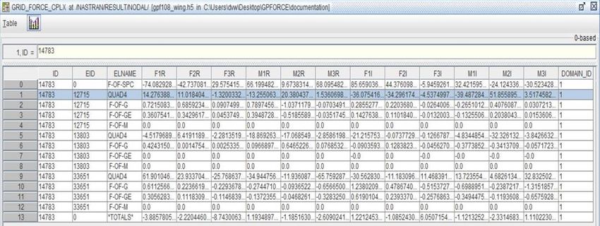
Feature Deprecation List

• Notice of features to be removed from MSC Nastran in 2020:
  • In an effort to streamline the MSC Nastran program and simplify ongoing maintenance activity, some
    obsolete capabilities have been identified and tagged for removal in a future release of the program in
    2021 and 2022, allowing for a reasonable notice period. Please review the list of features marked for
    deprecation below to ensure that there will be no disruption to your use of MSC Nastran. If you see a
    feature that you currently use and do not wish to lose, contact MSC Technical Support to report it.
• Features tagged for removal:
  • P-elements
  • SOL 600 nonlinear solution sequence – migration plan through 2021
  • Unstructured one- and two-digit solution sequences (e.g. SOL 3, SOL 24)
  • SOL 190 (DBTRANS)
  • TAUCS solver
  • MSGMESH
  • Obsolete DMAP modules
  • SSSALTERS
4   |   hexagonmi.com | mscsoftware.com
MSC Nastran Documentation

5   |   hexagonmi.com | mscsoftware.com
MSC Nastran 2020 Internal Webinar Agenda

           Introduction
           Dynamics                       Grid Point Forces in Frequency Response
                                          Rigid Elements TREF
                                          PEM Enhancements
                                          PEM Parallel Solution
                                          CDTire/NVH Linear Tire Model
                                          Coupled Modes for External Superelements
                                          Bent Rotor Modeling in Rotordynamics
           Fatigue                        CAEfatigue available in MSC Nastran
           Nonlinear SOL 400              Brake Squeal Enhancements
                                          Enhanced Segment to Segment Contact Settings
                                          ESE and EKE Output in SOL 400 Linear Perturbation Analysis
           HPC                            MUMPS Solver for SOL 101
           Results                        Eigenvector Output with Lossy Compression
           SOL 700                        DMP Support for Langrangian Solver

6   |   hexagonmi.com | mscsoftware.com
Dynamics

7   |   hexagonmi.com | mscsoftware.com
GPFORCE for Frequency
                                          Response Analysis

8   |   hexagonmi.com | mscsoftware.com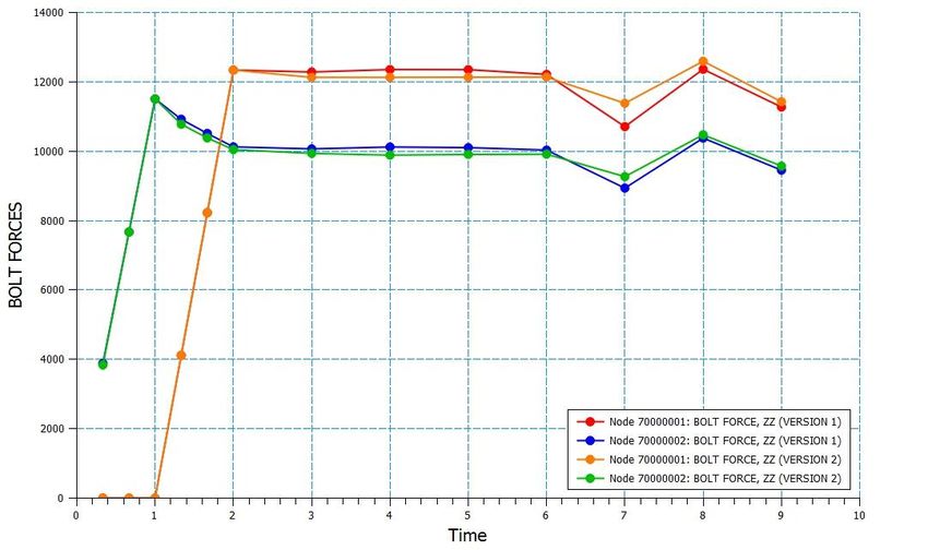
GPFORCE for Frequency Response Analysis
Overview

Introduction
• Extended GPFORCE options for explicit types of dynamic force output

Benefits
• Important frequency dependent element data recovery feature
  • Element force/stress recovery only performed at Master Frequencies for frequency dependent elements
  • Thermal loading is correctly accounted for

Use Case
• Load path analysis of structures – new for frequency response analysis
• Aerospace customer request
  • Also serves defense, transportation and security markets

9   |   hexagonmi.com | mscsoftware.com
GPFORCE for Frequency Response Analysis
Usage

•    ALLDLDS outputs everything – elastic, inertia, damping forces
•    Implemented in SOL108, SOL111 or ANALYSIS=DFREQ or MFREQ for SOL 200 and linear SOL 400
•    In general, for frequency response, the “*totals*“rows will not be zero, except when ALLDLDS is chosen
•    PARAM, BUSHNM, YES (default) required for GPFORCE.
•    GPFORCE is inherently a SORT1 output, SORT2 is suppressed

10   |   hexagonmi.com | mscsoftware.com
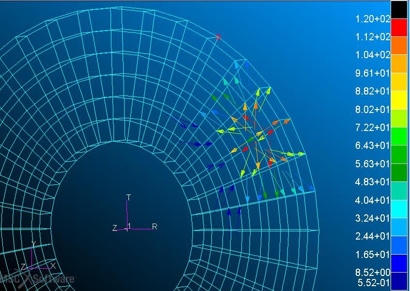
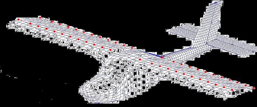
GPFORCE for Frequency Response Analysis
Example Model: (..\tpl\gpf_frq\gpf108_wing.dat)

                                                          GPFORCE(ALLDLDS)=2

                                                          GPFORCE=ALL option, large Grid IDs ≥
                                                          101000001 are from CWELD or CFAST or

                                                          CSEAM elements
                                                          SWLDPRM, PRTSW,n: To see connector grids

                                           SET 2 = 27188,20273,14783,113645,101002153,101002154

11   |   hexagonmi.com | mscsoftware.com
GPFORCE for Frequency Response Analysis
Example Output .f06
Elastic forces
Damping forces (G)
Structural damping
forces
Inertia forces (G)
…
Zero total (ALLDLDS requested)
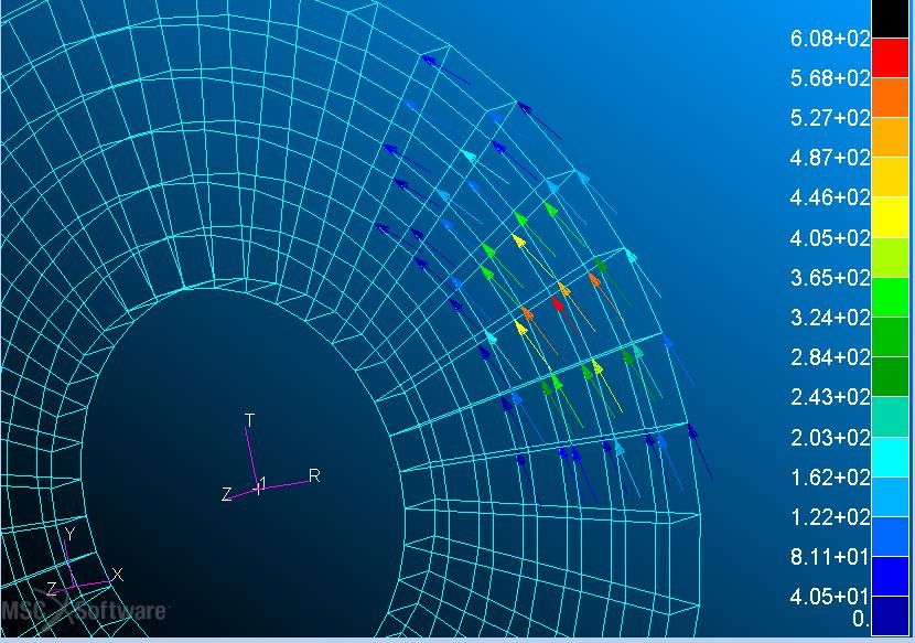
12 | hexagonmi.com | mscsoftware.comGPFORCE for Frequency Response Analysis
Example Output HDF5 – always stores in Real/Imaginary format
Grid ID Element ID Source
13 | hexagonmi.com | mscsoftware.comTREF Support for Rigid
Elements
14 | hexagonmi.com | mscsoftware.comTREF Support for Rigid Elements Overview Introduction • TREF support for rigid elements using TEMP(MATE) or TREF on elements (previously was zero) Benefits • TREF support removes a previous limitation (unwanted constraint) with modeling rigid elements in a temperature field • Now supported in all linear solutions sequences that allow thermal effects Use Case • In linear analysis with material dependency, rigid elements now reflect the local temperature field 15 | hexagonmi.com | mscsoftware.com
TREF Support for Rigid Elements
Usage

16   |   hexagonmi.com | mscsoftware.com
TREF Support for Rigid Elements
Usage

17   |   hexagonmi.com | mscsoftware.com
TREF Support for Rigid Elements
Usage

18   |   hexagonmi.com | mscsoftware.com
Porous Elastic Material
                                           Enhancements
                                           • Solid Shell using 3D Elements
                                           • Perforated Shell Elements
                                           • Simplified Biot Porous Material Models
                                           • Multiple Coupling Specifics for a Trim
                                             Component
                                           • TRMC Processing Scenarios
                                           • Rigid Elements for TRMC

19   |   hexagonmi.com | mscsoftware.com
Solid Shell Using 3D Elements 20 | hexagonmi.com | mscsoftware.com
Solid Shell Using 3D Elements
Overview

Introduction
• Solid shell is used to model transverse solid elements, with a thickness direction
• One dimension of the structure should be small compared with the two others (~ 1/15)
• Thickness (and thus compression effects) are accounted for using solid shells
Benefits
• New modeling feature
• For trim component only
• Isotropic materials only
Usage
• Hexa/Penta/Tetra/PYRAM element types can be used
• PSOLID entry FCTN field set to new PSLDSHL option (for PEM only)
• MID field points to MAT1 (not MATPE1)

             PSOLID                PID     MID   CORDM   IN   STRESS   ISOP     FCTN
             PSOLID                 1       1                                 PSLDSHL

21   |   hexagonmi.com | mscsoftware.com
Perforated Shell Elements 22 | hexagonmi.com | mscsoftware.com
Perforated Shell Elements
Overview

Introduction
• Perforated shells are common in many acoustic systems
   • Avoids fine meshing of holes
   • Not suitable for precision modeling of perforation

Benefit
• Reduce meshing effort
• Minimize CPU time

23   |   hexagonmi.com | mscsoftware.com
Perforated Shell Elements
Usage

• New MSC Nastran trim component bulk data entry PSHLPF
  • MID: solid material
  • T: thickness
  • SPACEG: spacing
  • RADIUS: radius
  • TOPOLGY: grid pattern (SQUARE / TRIA / HEXA)
  • FRHO: fluid density (air)
  • FVIS: viscosity
  • HOMG: homogenization (hole processing 0 or 1)

 PSHLPF                   PID              MID    T      SPACEG    RADIUS    TOPOLGY   FRHO    FVIS

                        HOMG

 PSHLPF                     1               2    8.1-4   1.132-2   1.245-3   SQUARE    1.225   1.71-5

24   |   hexagonmi.com | mscsoftware.com
Simplified Biot Porous Material
Model
25 | hexagonmi.com | mscsoftware.comSimplified Biot Porous Material Models Overview Introduction • Lumped porous • Model a porous medium when the material skeleton is assumed to be very soft (E=0) • Rigid porous • Model a porous medium when the material skeleton is assumed to be rigid • Delany-Bazley & Miki Porous • Semi-empirical numerical method for modeling porous materials • Assumes porosity = 1 • Only valid in a specific range (frequency/resistivity) Benefits • Easier modeling process for skeleton conditions • One dof per node in TRMC, instead of 4 • Potential performance improvement on TRMC matrix generation 26 | hexagonmi.com | mscsoftware.com
Simplified Biot Porous Material Models
Usage

• On the Nastran side for trim component
  • POROPT: porous options (LUMPED, RIGID, MIKI or DELANY)
         • MAT1 field must be left blank if POROPT is RIGID, MIKI or DELANY
         • MAT1 field can be used for POROPT=LUMPED to provide SRHO
         • MAT1 field must have valid input (integer>0) if POROPT is blank
     • SRHO: solid density for LUMPED porous only
     • VLE – Blank or 0.0 is acceptable(=>0.0, default=0.0)
     • TLE – Blank or 0.0 is acceptable(=>0.0, default=0.0)

 MATPE1                    MID             MAT1     MAT10    BIOT     POROPT   SRHO

                          VISC             GAMMA   PRANDTL   POR        TOR    AFR     VLE   TLE

 MATPE1                      1                       15               LUMPED    0.1

                         1.84-5                              9.4-1             4.0+4

27   |   hexagonmi.com | mscsoftware.com
Multiple Coupling Settings for
a Trim Component
28 | hexagonmi.com | mscsoftware.comMultiple Coupling Settings for a Trim Component Overview Introduction • Coupling specifics are provided on a set of ACPEMCP / TRMCPL entries • The distance between the structure or trim component and cavity can vary • A single set of ACPEMCP / TRMCPL may not be suitable for all regions of a trim component • REGION ID (RID) is implemented to handle diverse coupling conditions of a trim component Benefit • Coupling tolerances for a region of a trim component can be precisely defined • Better coupling between the structure or trim component and cavity without requiring model changes 29 | hexagonmi.com | mscsoftware.com
Multiple Coupling Settings for a Trim Component
Usage

• On Nastran side, for trim component
   • RID – region ID for ACPEMCP/TRMCPL (default=0)
   • ACPEMCP and TRMCPL with same TID and RID will be paired together
   • New design has minimum disturbance with existing PEM decks
   • FATAL if following conditions exist
      • TID,RID pair must be unique (trim and region IDs)
      • SET ID on ACPEMCP with different (TID,RID) pair must be different
      • OOC and SPM fields for RID>0 must be blank
 ACPEMCP                    TID             SGLUED   SSLIDE   SOPEN     SIMPER     OOC       SPM      SAIRGAP
                           SCUX              SCUY     SCUZ     SCRX      SCRY      SCRZ      SCFP       RID

 ACPEMCP                       1                      1002               1004
                                                                                                        20

     TRMCPL                  TID            CTYPE    PLTOL    GAPTOL1   GAPTOL2   GAPTOL3   GAPTOL4     RID

     TRMCPL                    1            SSLIDE    0.12       5                                      20

30    |   hexagonmi.com | mscsoftware.com
Trim Component Processing
Scenarios
31 | hexagonmi.com | mscsoftware.comTrim Component Processing Scenarios
Overview
Introduction
• Previously MSC Nastran supported:
• Processing of all trim components whether referenced by TRIMGRP Case Control or not
• MSC Nastran 2021 now supports ALLTRMC and SLTTRMC:
• New keywords on the TRIMGRP Case Control Example:
$ Sets for the TRIM 1 selection
• ALLTRMC – processes TRMC as with previous releases
SET 98 = 1
• SLTTRMC – processes selected TRMC only $ Sets for the TRIM 2 selection
SET 97 = 2
Benefit TRIMGRP(SLTTRMC)=98
• Processing referenced by TRMC only in Actran
• Performance improvements
32 | hexagonmi.com | mscsoftware.comRigid Elements for the Trim
Component
33 | hexagonmi.com | mscsoftware.comRigid Elements for the Trim Component Overview • In previous releases of MSC Nastran • Rigid elements under BEGIN TRMC=TRMID were ignored • For MSC Nastran 2021 • RBE2 / RBE3 elements are processed as part of the TRMC model in Actran 34 | hexagonmi.com | mscsoftware.com
New Parallel Solution for
                                           MSC Nastran-PEM

35   |   hexagonmi.com | mscsoftware.com
New Parallel Solution for MSC Nastran-PEM Overview • Nastran/PEM analysis of large models with many trim components expose limitations to Nastran DMP • Primary use case: automotive model with several trim components, for example • 10 trim components • 20 – 30 trim master frequencies • 15 – 20 panels defined for panel participation • PEM-related operations computed on Master DMP process only, even in DMP mode • Based on DMP Master-Slave approach • Unacceptable runtime 36 | hexagonmi.com | mscsoftware.com
New Parallel Solution for MSC Nastran-PEM
Overview
Example compute profile using DMP=2
 Step                       Computation          Percent of Total

            1               Nastran phase 1              1.0

            2               Modal reduction              2.7        Increasing DMP value has no effect
                                                                    on performance
            3               Frequency response           0.1

            4               Actran                       9.6

            5               Import RIM                   8.0                         Serial
            6               Acoustic coupling           29.7                         processing
            7               PPF coupling                46.5                         (SMP only)
            8               PPF calculation              0.8

            9               Other                        0.9

37   |   hexagonmi.com | mscsoftware.com
DMP=2 example • Trim Master Frequencies are evenly
Forcing Frequencies (241)
Master: 101 from 10-110 distributed to DMP processes
Slave: 140 from 111-250 • Corresponding forcing frequencies
Trim Master Frequencies (22) may be unbalanced
Master: 12 from 10-120
Slave: 12 from 110-260 • This is OK if the cost per forcing
frequency is small
38 | hexagonmi.com | mscsoftware.comNew Parallel Solution for MSC Nastran-PEM
Usage
• REQUIRED: PARAM,PEMDMP,YES in bulk data
• User must specify dmp=N (N>1) on command line
• If multiple hosts are used, no additional input is required
• Specify multiple hosts on command line, for example: host=host1:host2
• If using a single host, specify the RUNOPT keyword on DOMAINSOLVER
• DOMAINSOLVER ACMS (RUNOPT=MULTIMST, …)
• When PEMDMP is activated, User Information Messages 10544 and 10545 are printed in F06 file:
*** USER INFORMATION MESSAGE 10544 (MTMD62)
TOTAL NUMBER OF FORCING FREQUENCIES: 481 - MIN FORCING FREQUENCY: 20.00 - MAX FORCING FREQUENCY: 500.00
TOTAL NUMBER OF TRIM MASTER FREQUENCIES: 25 - MIN TRIM MASTER FREQUENCY: 20.00 - MAX TRIM MASTER FREQUENCY: 500.00
*** USER INFORMATION MESSAGE 10545 (MTMD62)
PROCESS ID NUMBER OF TRIM MASTER FREQUENCIES (MIN - MAX) NUMBER OF FORCING FREQUENCIES (MIN - MAX)
1 14 20.00 ( 1) - 280.00 ( 14) 241 20.00 ( 1) - 260.00 ( 241)
2 13 260.00 ( 13) - 500.00 ( 25) 240 261.00 ( 242) - 500.00 ( 481)
39 | hexagonmi.com | mscsoftware.comNew Parallel Solution for MSC Nastran-PEM
Example: PEMDMP Test Case from Auto Industry Machine characteristics
• Linux RH7.5
Model description • 512GB main memory
• 3.4 million grid points; 20.0 million DOF; structure A-size 15.5 million DOF • IntelR XeonR Gold 6126 CPU @
• Eigenvalues: 2400 up to 400Hz (structure) – 300 up to 800Hz (fluid) 2.6.0GHz
• 241 forcing frequencies from 10Hz to 250Hz @1Hz • Jobs were run using 200gb memory
and 8 cores per DMP process
• 9 trim components – 22 trim master frequencies
(smp=8).
• 17 panels
Elapsed Time (hours)
Version Elapsed Time Disk I/O Max Disk 25
20
2020.0 DMP=2 1271:34 (21h 11m) 25.0 TB 2.0 TB
15
2021.0 DMP=2 784:09 (13h 4m) 29.4 TB 2.3 TB
(14.7TB/host) (1.1TB/host) 10
2021.0 DMP=3 603:22 (10h 3m) 28.6 TB 2.7 TB
5
(9.8TB/host) (0.9TB/host)
2021.0 DMP=4 512:37 (8h 32m) 31.0 TB 2.8 TB 0
(7.7TB/host) (0.7TB/host) DMP=2 DMP=2 DMP=3 DMP=4
V2020.0 V2021.0
40 | hexagonmi.com | mscsoftware.comHigh-Fidelity Tire Modeling
with CDTire/NVH
41 | hexagonmi.com | mscsoftware.comHigh-Fidelity Tire Modeling with CDTire/NVH
Overview
Introduction
• CDTire is a popular 3-D tire simulation model family used in the automotive industry:
• Modelling and parameterization of all functional layers of a modern tire
• Accurate modelling acoustic cavity and gyroscopic effects of rolling tire
• CDTire has introduced a linearized tire capability called CDTire/NVH:
• The linearized tire matrices are exported around a particular operating condition
(tire rotation speed, inflation pressure, preload, contact patch discretization, etc.)
of interest to the simulation engineer
• Linearized tire matrices and associated model information are exported for direct
inclusion in MSC Nastran
42 | hexagonmi.com | mscsoftware.comHigh-Fidelity Tire Modeling with CDTire/NVH Overview • MSC Nastran 2021 enables the use of CDTire/NVH tire models in the following solutions: • SOL 103: Normal modes • SOL 107, Sol 110: Direct and Modal Complex modes • SOL 108, 111: Direct and Modal Frequency response • SOL 109, 112: Direct and Modal Transient response • SOL 200 Analysis • SOL 400 Linear • Typical Applications: • NVH analysis using transient and frequency response simulation • Ride Comfort studies on digitized road surfaces • Harshness analysis on artificial obstacles (cleats) 43 | hexagonmi.com | mscsoftware.com
High-Fidelity Tire Modeling with CDTire/NVH
Overview

Benefits
• Accurate NVH simulation require high fidelity tire models
  • Particularly with electric cars (eNVH) where road noise is more apparent
• Previously MSC Nastran users have employed modal tire model provided by the tire manufacturers - modal tires have
  a few drawbacks:
  • Cannot change boundary conditions or operating conditions
  • Gyroscopic effects and acoustic cavity are not modeled
• Tire Models are expensive to generate and automobile manufacturers already use them in their vehicle handling
  simulations
  • The same models can now be used for NVH simulations in MSC Nastran

Licensing
• Fraunhofer license required for CDTire/NVH
• Separate MSC Nastran license feature NA_Tire_Modeling

44   |   hexagonmi.com | mscsoftware.com
High-Fidelity Tire Modeling with CDTire/NVH
Workflow
                                                                     CDTire/NVH Generator
Tire model generation
• CDTire/NVH tire models consist of two ASCII files meant for
   direct inclusion in the Nastran input file:
   • XXX_GRID.dat : Which has the associated tire model
      information containing GRIDs/SPOINTs, RBE2s, CORD1R
      and PLOTELs. To position the tire within the vehicle the
      interface grids (wheel center, Z-Axis and X-Axis grids) need
      to be repositioned by the user
   • XXX_DMIG.dat : The linearized tire system matrices, i.e.,
      mass, damping and stiffness matrices. These matrices are
      exported in Nastran DMIG format

45   |   hexagonmi.com | mscsoftware.com
High-Fidelity Tire Modeling with CDTire/NVH
Workflow
CDTire/NVH Generator
creates the linearized CDTire/NVH Tire Model
representation of the
tire at a particular XXX_GRID.dat: tire model information
operating condition XXX_DMIG.dat: linearized tire matrices
MSC Nastran SOL 103, 107/110,
NVH analysis
model with tire 108/111, 109/112, SOL 200
definition and SOL 400 Linear
46 | hexagonmi.com | mscsoftware.comCoupled Modes Support for
External Superelements
47 | hexagonmi.com | mscsoftware.comCoupled Modes Support for External Superelements
Overview
Introduction
• A coupling surface exists between the solid mesh of a fluid cavity and the structural elements
• The vibrating structure defines a velocity boundary condition on the fluid
• The acoustic pressure in the fluid defines a pressure load on the structure
Structure
• Some considerations
• A fluid completely enclosed by a structure has a stiffening effect on it Fluid cavity
• The inertia of the fluid increases the mass of the structure
• For gas cavities, these effects are small and allow uncoupled analysis
• For heavy fluids (gasoline, water,…) these effects cannot be ignored
• The coupling appears in K and M matrices rendering them asymmetric
• External superelements in a dynamic analysis
• Component mode synthesis (CMS) is needed to obtain results for the final assembly run
• A new capability allows coupled modes to be computed for the CMS phase of the external superelement generation
Benefits
• Real coupled modes for the CMS also supports ADAMSMNF
• Analysis of launch vehicles and tanks filled with heavy fluid, i.e. liquids
48 | hexagonmi.com | mscsoftware.comCoupled Modes Support for External Superelements
Usage Acoustic pressure at point id =158721
3.00E-05
• EXTSE creation with coupled modes. 2.50E-05
2.00E-05
• Standard EXTSEOUT case control format
• METHOD(COUPLED) = setid 1.50E-05
Displacement
• SDAMPING(COUPLED) = tabid 1.00E-05
5.00E-06
• Bulk Card entry
• EIGR/EIGRL with V1,V2,ND 0.00E+00
1.00E+01 2.00E+01 3.00E+01 4.00E+01 5.00E+01 6.00E+01 7.00E+01
• PARAM,SESDAMP, AUG (recommended) –
-5.00E-06
for SDAMPING(coupled)
• Standard TABDMP1 -1.00E-05
Freq
• ASETi/BSETi/ACCSSPT (fixed boundary)
oil_tank_SE108 oil_tank_noSE108
49 | hexagonmi.com | mscsoftware.comExternal Superelements with
Monitor Points
50 | hexagonmi.com | mscsoftware.comExternal Superelements with Monitor Points Overview Introduction • Enhancement combines two powerful capabilities • External superelements • Monitor points • For example: • A subcontractor can define monitor points in an external superelement • The general contractor can compute the monitor point responses in the assembly run Usage • No new Case Control or Bulk Data entries required • In the external superelement creation run the user specifies: • MONITOR and EXTSEOUT Case Control commands • Bulk Data entries: MONDSP1, MONPNT1, MONPNT2, MONPNT3, MONSUM, MONSUMT and MONSUM1 • In the assembly run the user needs to specify the MONITOR Case Control command to obtain the monitor point results for the external superelement 51 | hexagonmi.com | mscsoftware.com
External Superelements with Monitor Points
Example

• Simulated Rocket Example
  • Simple Cylinder 10 units long comprises the external
    superelement 55
  • Boundary grids form the residual structure and are located at
    every 2.5 units along centerline and connected by rigid
    spiders (5 stations at 0.0, 2.5, 5.0, 7.5, 10.0 units)

•        Generation of MONPNT3 input for Section Loads using Patran
         Flight Loads option
          • Select “MonPt” location (node at centerline)
          • Select Nodes for section cut
          • Select elements on one side of section cut

52   |    hexagonmi.com | mscsoftware.com
External Superelements with Monitor Points
Example
• Assembly run f06 excerpt showing station cut loads at 2.5 units for external superelement 55
• Monitor point results are also written to op2 and hdf5 if requested
SUPERELEMENT 55
S T R U C T U R A L I N T E G R A T E D F R E E B O D Y M O N I T O R P O I N T L O A D S
(MONPNT3)
MONITOR POINT NAME = STA2.5 SUBCASE NO. 1
LABEL = STATION 2.5 SECTION LOADS
CP = 0 X = 2.50000E+00 Y = 0.00000E+00 Z = 0.00000E+00 CD =
0
AXIS REST. APPLIED AXIS REST. APPLIED
---- ------------- ---- -------------
CX -2.089855E-06 CX -2.090819E-06
CY 5.765389E-03 CY 5.765406E-03
CZ -3.563133E-03 CZ -3.563134E-03
Internal Superelement Results
CMX 5.340617E-03 CMX 5.340590E-03
CMY -4.973561E-03 CMY -4.973563E-03
CMZ -8.129106E-03 CMZ -8.129109E-03
53 | hexagonmi.com | mscsoftware.comBent Rotor Modeling in
Rotordynamics
54 | hexagonmi.com | mscsoftware.comBent Rotor Modeling in Rotordynamics Overview Introduction • In reality, there are imperfections, manufacturing tolerances, that cause rotor geometry to be susceptible to bends, kinks and offsets • MSC Nastran 2021 introduces a new feature to model the imperfect geometry of a rotor • New ROTBENT Case Control command and Bulk Data entry in SOL 400 • Current implementation is for line rotors (1D line elements) modeled as 3D rotors using the ROTOR entry Workflow – two steps in SOL 400 • Step 1 – static analysis • Model the rotor as straight • Use ROTBENT bulk data entry to model the imperfections (kinks and offsets) and bearing connections • MSC Nastran will update the rotor geometry effectively pulling the rotor into the bearings and making the connection • Step 2 – complex eigenvalue analysis or frequency response using the solution of Step 1 as a starting point • Complex eigenvalues includes Campbell diagrams • Frequency response includes dynamic application of the forces due to pulling the rotor into the bearings 55 | hexagonmi.com | mscsoftware.com
Bent Rotor Modeling in Rotordynamics
Example – Executive and Case Control

SOL 400
CEND
RIGID=LINEAR $ optional
rotbent=1
SPC = 10 $ SPC’s holding stator to ground (The ROTBENT will create SPC’s, MPC’s, and SPCD’s pulling the rotor into the bearings)
subcase 1
 step 1 $ static solution to pull rotor into bearings
    nlparm=1
    analysis=nlstat $ first step is the static solution
    load = 1 $ point to LOAD ID on ROTBENT in bulk data for static loads pulling rotor into bearings
 step 2 $ Rotordynamics solution
    label = complex eigenvalues $ can be complex modes or frequency response
    ANALYSIS=dceig
    cmethod = 1
    RGYRO= 100
    NLIC = 1 $ use results of STEP 1 as the starting point
56   |   hexagonmi.com | mscsoftware.com
Bent Rotor Modeling in Rotordynamics Example – Bulk Data For this example, let us assume we have a rotor which is parallel to the BASIC X axis and we wish the ROTOR Y-axis to be parallel to the BASIC Y (Rotor system parallel to basic system) Bulk data Input (For this example, all GRID points use BASIC as CD): rotbent,1,10,3 $ ROTBENT 1, for ROTOR 10, creates loads for LOAD=3 ,unbcord,0. ,1.,0. $ rotor XY plane – in the CD of the first GRID on the AXIS list ,offset,1.1,.1,0. ,,2.1,.2,90. ,,3.1,.3,180. ,brgdpr,1,101 $ bearing pairs: rotor grid to stator grid ,,10,110 57 | hexagonmi.com | mscsoftware.com
Bent Rotor Modeling in Rotordynamics
Example

                                                                K&O                                                                    After Pulling into Bearings
                       0.002                                                                                        0.0025

                           0                                                                                         0.002
                       -0.002                                                          T2
                                                                                                                    0.0015                                                 T1
                                                                                       T3
                       -0.004                                                                                                                                              T3
                                                                                       BRG                           0.001
     Deformation, in

                                                                                                  Deformation, in
                       -0.006                                                                                                                                              BRG
                                                                                                                    0.0005
                       -0.008
                                                                                                                         0
                        -0.01
                                                                                                                    -0.0005
                       -0.012
                                                                                                                     -0.001
                       -0.014

                       -0.016                                                                                       -0.0015

                       -0.018                                                                                        -0.002

                        -0.02                                                                                       -0.0025
                                0          10              20         30     40   50         60                               0   10          20       30        40   50         60
                                                                  Axis, in                                                                           Axis, in

58                 |     hexagonmi.com | mscsoftware.com
Bent Rotor Modeling in Rotordynamics
Example
Unbalance Response with Kinks and Offsets Response - Kink&Offset Only
0.0035 0.000008
0.003 0.000007
Node 4 Node 4
0.000006
0.0025 Node 15 Node 15
Amplitude, in
Amplitude, in
0.000005
0.002
0.000004
0.0015
0.000003
0.001
0.000002
0.0005 0.000001
0 0
0.0 50.0 100.0 150.0 200.0 250.0 300.0 350.0 0.0 50.0 100.0 150.0 200.0 250.0 300.0 350.0
Freq, Hz Freq, Hz
59 | hexagonmi.com | mscsoftware.comFatigue:
CAEfatigue in MSC Nastran
60 | hexagonmi.com | mscsoftware.comCAEfatigue Software (Cf)
Updating current NEF and NEVF over 3 release cycles through June 2021
3 Software Packages
4 Technologies
For Fatigue, Random Response,
Loads Management and
Test Design
Frequency Premium Test
Premium Full Body
Time
61 | hexagonmi.com | mscsoftware.comCAEfatigue Software (Cf)
The Vision for Alignment with MSC Software / Hexagon
One unified Durability, Random Response and Loads Management offering
Cf Cf Cf
TIME FREQUENCY PREMIUM
Solver Linked MSC One Apex Aligned
(Nastran, Marc)
Supports Nastran,
Optistruct, Ansys, Abaqus
62 | hexagonmi.com | mscsoftware.comCAEfatigue in MSC Nastran
Roadmap through mid-2021
• MSC Nastran 2021 (December 2020)
• All Time Domain updated except items listed on next slide
• MSC One licensing added to both Time Domain (NEF) and Frequency Domain (NEVF) solvers
• CAEfatigue is now the default NEF and NEVF technology
• MSC Nastran 2021.1 (March 2021)
• Time Domain update will be completed
• MSC Nastran 2021.2 (June 2021)
• Frequency Domain update will be completed with the addition of a “Random” solver (MSC Random inside
Nastran!)
63 | hexagonmi.com | mscsoftware.comCAEfatigue in MSC Nastran
CAEfatigue Limitations in MSC Nastran 2021
Case or Bulk Data Non-Supported Entries
FATIGUE FORMAT=1,2,4,16, 32 or any bit combination that contains these values
STROUT=4
HISTOGRAM Just the existence
FTGDEF TOPSTR
TOPDMG
SPOTW or SEAMW {of any kind}
FTGPARM PLAST=SEEGER
INTERP
RAINFLOW
FOS
DAMAGE
SPOTW or SEAMW
MULTI
COMB=VONMIS,MAXPRINC,SGMAXSHR,MAXSH,COMPX/Y/Z/XY/YZ/ZX
CORR=FKM,INTERP
FTGSEQ METHOD=1 or 2, nested FTGSEQ
PFTG Non default
MATFTG STATIC CODE>=200, RR != default
SN MSS
BASTEN
TABLE - more than one!
64 | hexagonmi.com | mscsoftware.com TABLRPC
The existence of TABLRPCCAEfatigue in MSC Nastran
Performance Improvements
• Great strides continue to be made in improvements to Nastran Embedded Fatigue (NEF) time-based fatigue analysis
performance.
• In the previous release, performance improvements to fatigue analysis using SOL 112 (modal transient analysis) with
load sequences using multiple events (Duty Cycles) was introduced
• In this release, more algorithm improvements have been made (by incorporating CAEfatigue technology) to speed
up all time-based fatigue analyses using SOL 101, 103, and 112.
• The magnitude of the performance increase is dependent on the complexity of the analysis, favoring large models
with complex and long loading histories, such as the road load data used for typical automotive vehicle duty cycles
65 | hexagonmi.com | mscsoftware.comCAEfatigue in MSC Nastran Performance Improvements • The performance improvements are applicable to standard S-N and e-N analysis • Improvements to other fatigue analysis types such as Spot Weld, Seam Weld, Factor of Safety, Multi-axial Assessment, 3-pass (hot spot) and frequency domain are planned for future releases 66 | hexagonmi.com | mscsoftware.com
CAEfatigue in MSC Nastran
Performance Improvements

67   |   hexagonmi.com | mscsoftware.com
Nonlinear SOL 400

68   |   hexagonmi.com | mscsoftware.com
Brake Squeal Enhancements

69   |   hexagonmi.com | mscsoftware.com
Brake Squeal Enhancements
Overview

Introduction
• Brake squeal is induced from the sliding friction
   contact between the rotating disk and static pads
• Also influences the deformation of the brake
   system and other parts of the structure

Limitations of current capability
• Multiple wheels / axes are not supported
• Can’t specify brake / disk pair – all touching
  contact pairs are treated as part of the brake
• Drum brakes not supported
• Disk rotation effects are not included

70   |   hexagonmi.com | mscsoftware.com
Brake Squeal Enhancements
Overview

Benefits
• In MSC Nastran 2021 all previous limitations are removed
  • NLSTAT enhanced to include disk rotation effect
  • Multiple wheels / axes supported
  • Drum brakes supported
  • Explicitly define brake contact pairs
• Translational movement definition added
• Supporting users to determine the touching contact status
  during the linear perturbation and ignoring the status
  obtained by nonlinear static analysis

71   |   hexagonmi.com | mscsoftware.com
Brake Squeal Enhancements
Example
                                           Disk (Rotor)
• Model
  • (brksys5a wo sliding)
                                           Pads
  • (brksys3a w sliding)

                                           Pistons

72   |   hexagonmi.com | mscsoftware.com
Brake Squeal Enhancements
Example: Friction force
Disk No Sliding Disk Sliding
73 | hexagonmi.com | mscsoftware.comBrake Squeal Enhancements
Example: Eigenvalue Output
Disk No Sliding
Disk Sliding
74 | hexagonmi.com | mscsoftware.comBrake Squeal Enhancements
Example: Eigenvectors
1st mode 2nd mode
No Sliding
Sliding
75 | hexagonmi.com | mscsoftware.comBrake Squeal Enhancements
Other Applications
Squeal analysis of windshield wipers Translation movement in motion squeal
analysis and general contact analysis
76 | hexagonmi.com | mscsoftware.comSegment-to-Segment Contact
Enhancements
77 | hexagonmi.com | mscsoftware.comSegment-to-Segment Contact Enhancements Overview Feedback • Node-to-seg converges, but seg-to-seg doesn’t • Seg-to-seg in Marc converges, but SOL 400 doesn’t • SOL 400 requires more iterations than Marc • Seg-to-seg is unstable in different releases Objective with MSC Nastran 2021 • Improve seg-to-seg robustness • Improve consistency compared with Marc Implementation • Change default settings in seg-to-seg contact • Activate enhanced algorithm from contact component in Marc 78 | hexagonmi.com | mscsoftware.com
Segment-to-Segment Contact Enhancements
Enhancement

List of enhanced items to improve performance and robustness of seg-to-seg method

• Ramping down penalty when angle between segment normals below minimum segment angle

• Evaluate contact matrix/force based upon true updated patch coordinates

• New patch sequence renumbering algorithm based upon patch geometry

• Reset iteration count after separation

• New logic in creating polygons under sliding condition

• Scaled incremental displacement update in large rotation scheme

79   |   hexagonmi.com | mscsoftware.com
Segment-to-Segment Contact Enhancements
Usage

 BCPARA                    0                       METHOD            SEGTOSEG        VERSION          1 OR 2           BACKCTL            0 TO 63

 VERSION                                   Defaults version control in Segment-to-Segment method

                                           1             Version 1

                                           2 (default)   Version 2 (lower penalty, recommended)

 BACKCTL                                   Backward compatible bit-wise control in seg-to-seg contact analysis (0 default)

                                           1             Body order independent and ramping down penalty below minimum seg angle

                                           2             Old evaluation of contact matrix/force on patch coordinates (back to 2020 SP1)

                                           4             Old patch sequence renumbering (back to 2020 SP1)

                                           8             No reset iteration count after separation (back to 2020 SP1, Version 2 only)

                                           16            Old logic in creating new polygons (back to 2020 SP1)

                                           32            Scaled incremental displacement update in small rotation (back to 2020 SP1)

80   |   hexagonmi.com | mscsoftware.com
Segment-to-Segment Contact Enhancements
Example Benchmark
158,600 NODEs
101,970 TETRAs
2 Bolts
5 Contact Bodies
9 STEPs mechanical+thermal load
3 increments for 1st and 2nd STEP
1 increment for the rest STEPs
CONV=PV EPSP=5.0E-2
Nastran 2020 (Version 2) Total Iteration 270
Nastran 2021 beta (Version 2) Total Iteration 88
Nastran 2021 beta (Version 1) Total Iteration 112
Nastran 2021 beta (Version 2) Total Iteration 103
1 increment for all 9 STEPs
CONV=PV EPSP=1.0E-2
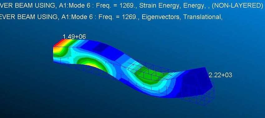
81 | hexagonmi.com | mscsoftware.comESE and EKE in SOL 400 Multi-
disciplinary and Linear
Perturbation Analyses
82 | hexagonmi.com | mscsoftware.comESE and EKE in SOL 400 Overview Introduction • Element Strain Energy (ESE) and Element Kinetic Energy (EKE) computations have been traditionally supported for linear Nastran elements in linear analyses such as static, transient and modal analyses • Users have requested ESE and EKE support in Nastran SOL 400 linear perturbation analysis using normal modes (MODES) and modal complex eigenvalue (MCEIG) analyses • This release introduces ESE and EKE support in Nastran SOL 400 multi-disciplinary and linear perturbation analyses using MODES and MCEIG analyses and includes support for advanced nonlinear elements Benefits • Strain energy density gives analysts insight into the regions in the model that have the greatest deformation • Strain energy density is a very good indicator for load paths, fracture, damage and fatigue prediction; elements located on a load path work harder than others • Topology optimization may involve an evaluation of the strain energy density for several modes then removing material from regions with low strain energy density and adding material to regions of high strain energy density • Kinetic energy density can help locate where to place dynamic vibration absorbers in a structure; vibration absorbers are typically placed in regions with high kinetic energy density • ESE and EKE computations in modal analyses also reveal the modal energy contributions of a particular mode 83 | hexagonmi.com | mscsoftware.com
ESE and EKE in SOL 400
Overview

Usage
• Existing Case Control commands are used to request ESE and EKE output in SOL 400 multi-disciplinary and linear
  perturbation analyses
• User can select ALL elements or a subset of elements for output
• Output includes element strain / kinetic energy, element strain / kinetic energy density and percent of model total
• For modal complex eigenvalue analysis, AVERAGE, AMPLITUDE and PEAK values of ESE and EKE are supported,
  AVERAGE is the default
• Results may be output to the F06, OP2 and/or H5 files for the selected elements for each mode

84   |   hexagonmi.com | mscsoftware.com
HPC:
                                           MUMPS Solver in Linear
                                           Statics

85   |   hexagonmi.com | mscsoftware.com
MUMPS Solver in Linear Statics Overview Introduction • Solution of linear equations comprises more than 60% of the elapsed time in SOL 101 • Problem size ranges from 10M to 50M dof and extending to 300M dof in the future • Multi-frontal direct solvers (like MUMPS) require 5x-7x higher memory than frontal direct and iterative solvers • Need for distributed memory direct solver in MSC Nastran Benefits • Less memory required per machine / host via DMP compared to MKL Pardiso • Scale out capability across multiple machines / hosts Current limitations • Inertia relief -1, -2 is not supported • SOL 101 jobs involving linear contact is not supported • Only in-core is supported • Windows platform is not supported 86 | hexagonmi.com | mscsoftware.com
MUMPS Solver in Linear Statics
Usage

Input
• Invoke MUMPS Solver by using the SPARSESOLVER executive control statement
• Only DCMP module of SPARSESOLVER statement is supported.

                                           SOL 101
                                           SPARSESOLVER DCMP(FACTMETH=mumps)
                                           CEND

Output in F04

87   |   hexagonmi.com | mscsoftware.com
MUMPS Solver in Linear Statics
Performance Results
Solver Performance Comparison
300 274
250
Elapsed time in minutes
200
172
50m dof (shell elements) 150
Pardiso
100
Mumps
43 39 44
50 30 33 35 27
0
• MUMPS scalability slightly better in most of the above configurations
• DMP=4 and SMP=8, MKL Pardiso’s in-core memory requirement is higher than available physical memory on the
machines, whereas MUMPS ran successfully and showed further scalability on the same machines because of its
lower memory requirement per machine/host
88 | hexagonmi.com | mscsoftware.comResults:
Eigenvector Output with Lossy
Compression
89 | hexagonmi.com | mscsoftware.comEigenvector Output with Lossy Compression
Overview
Introduction
• New lossy compression support in MSC Nastran 2021
• NLOUT output
• Monitor point output
• Included support for more data types
• Brake squeal, temperature dependent entries, GPFORCE, PACCELERATION
Benefits
• Improve NH5RDB performance
• Store data more efficiently
• Enhanced data structures improve post-processing applications (indexing)
90 | hexagonmi.com | mscsoftware.comNH5RDB
Compression in NH5RDB
• Current compression – Gzip compressor
• Lossless compression
• Applied to compound data – Tables
• All datasets in current NH5RDB are defined as compound types
• Data structure with integers, characters and floating-point numbers
• New lossy compression support – Scaleoffset Compressor
• Applied on matrix
• Floating-point numbers only
• Support multiple dimensional array
• Define floating point number array type dataset
91 | hexagonmi.com | mscsoftware.comNH5RDB
NH5RDB Schema Update
• NH5RDB schema is extended to support lossy compression definition
• Add scaleoffset attribute for lossy compression definition
• Support compression factor option in model
• Add MDLPRM parameters for compression option in input file
• For example, use factor 3 (default) for defined dataset with scaleoffset compressor: MDLPRM, H5SGENL,3
• Factor ranges from -1 to 10
• 0 to 10 : scale factor with lossy compression
• -1: Use lossless compression
Compression Dataset Compression
Example: Method Size (MB) Ratio
• Eigenvector matrix output Scaleoffset, factor = 3 129 4.75
• DOF number = 220,698, Eigenvector number = 364 Scaleoffset, factor = 4 160 3.84
• Matrix data size: 220,698 x 364 x 8 = 612 MB Scaleoffset, factor = 5 190 3.22
• Run with different factors for lossy compression Scaleoffset, factor = 6 221 2.77
and lossless compression Gzip, level = 1 584 1.05
92 | hexagonmi.com | mscsoftware.comSOL 700 / Dytran:
DMP Support for Lagrangian
Solver
93 | hexagonmi.com | mscsoftware.comDistributed Memory Parallel (DMP) for Structural Solver in SOL 700
Overview
Introduction
• DMP was already implemented for the Eulerian (fluid) solver
• MSC Nastran 2021 introduces the DMP for the Lagrangian (structural) solver
Cores Performance
1 1.00
2 2.05
4 4.01
8 7.27
16 11.25
32 17.64
Benefits
• Performance improvements for large models on machines with multiple cores and/or clusters of multiple nodes
• Initial focus is on quality, subsequent releases will optimize MPI calls and load balancing
94 | hexagonmi.com | mscsoftware.comDistributed Memory Parallel (DMP) for Structural Solver in SOL 700
Usage
• Any explicit model with a large number of structural elements
• Limitations:
• Contact serial only under DMP run
• Rigid bodies and rigid connections are calculated in the Master CPU only under DMP run
• Contact options BELT/BELT1/DRAWBEAD not supported
• Older Contact Version 2 not supported
• ATB dummies not supported
• IMM (Initial Metric Method) for air bag simulations not supported
• Nastran prestress
• Control DMP with DYPARAM, DMPOPT:
• FSI DMP but not Structure
• Structure DMP but not FSI
• FSI and Structure DMP
95 | hexagonmi.com | mscsoftware.comDistributed Memory Parallel (DMP) for Structural Solver in SOL 700
Further Details
• Performance improvements are especially expected under the following circumstances when the serial has:
1. High elapsed time per cycle: Time/Cycle > 0.1 seconds
2. No or low contact (contact is running serial)
3. At least 2,000 elements per core (performance gains outweighing MPI communications)
4. Low number of properties and element types (load balancing and MPI call optimizations is work in progress)
96 | hexagonmi.com | mscsoftware.comDistributed Memory Parallel (DMP) for Structural Solver in SOL 700
Performance
• Example 1: Cores Performance
1 1.00
2 1.97
535,416 solid elements 4 3.62
Contact in Serial: 0.28% 8 6.25
16 9.22
Time per cycle: 0.178 seconds 32 12.89
• Example 2: Cores Performance
1 1.00
2 1.93
165,000 solid / shell elements 4 3.33
Contact in Serial: 2.4% 8 5.41
16 7.23
Time per cycle: 0.06 seconds 32 9.43
97 | hexagonmi.com | mscsoftware.comThank You! 98 | hexagonmi.com | mscsoftware.com
You can also read