Modeling Savings for ENERGY STAR Smart Home Energy Management Systems - July 2021
←
→
Page content transcription
If your browser does not render page correctly, please read the page content below
Modeling Savings for ENERGY STAR
Smart Home Energy Management
Systems

July 2021

Disclaimer
This work was prepared as an account of work sponsored by an agency of the United States
Government. Neither the United States Government nor any agency thereof, nor any of their
employees, nor any of their contractors, subcontractors or their employees, makes any warranty,
express or implied, or assumes any legal liability or responsibility for the accuracy,
completeness, or any third party’s use or the results of such use of any information, apparatus,
product, or process disclosed, or represents that its use would not infringe privately owned rights.
Reference herein to any specific commercial product, process, or service by trade name,
trademark, manufacturer, or otherwise, does not necessarily constitute or imply its endorsement,
recommendation, or favoring by the United States Government or any agency thereof or its
contractors or subcontractors. The views and opinions of authors expressed herein do not
necessarily state or reflect those of the United States Government or any agency thereof, its
contractors or subcontractors.

Available electronically at Office of Scientific and Technical Information website (osti.gov)
Available for a processing fee to U.S. Department of Energy
and its contractors, in paper, from:
U.S. Department of Energy
Office of Scientific and Technical Information
P.O. Box 62
Oak Ridge, TN 37831-0062
OSTI osti.gov
Phone: 865.576.8401
Fax: 865.576.5728
Email: reports@osti.gov
Available for sale to the public, in paper, from:
U.S. Department of Commerce
National Technical Information Service
5301 Shawnee Road
Alexandria, VA 22312
NTIS ntis.gov
Phone: 800.553.6847 or 703.605.6000
Fax: 703.605.6900
Email: orders@ntis.gov

                                                       ii
Modeling Savings for ENERGY STAR Smart Home Energy
                  Management Systems

                               Prepared by:
    Robert Hendron, Kristin Heinemeier, Alea German, and Joshua Pereira
                              Frontier Energy

                              Prepared for:
                       Building Technologies Office
             Office of Energy Efficiency and Renewable Energy
                        U.S. Department of Energy

                                July 2021

                 NREL Technical Monitor: Conor Dennehy

                                    iii
Acknowledgments
The authors acknowledge the financial resources and valuable input provided by the National
Renewable Energy Laboratory, including Stacey Rothgeb, Conor Dennehy, Lena Burkett, and
Lieko Earle. The ENERGY STAR® Smart Thermostat and Smart Home Energy Management
System team (Abigail Daken, Theo Keeley LeClaire, and Taylor Jantz-Sell) provided important
insights that were used to guide the technical approach. Several experts on home energy
management and demand response programs provided information from previous studies,
including Albert Chiu of Pacific Gas and Electric, Kitty Wang of Energy Solutions, and Dr.
Farhad Omar of the National Institute of Standards and Technology. We also recognize the
important contributions made by other members of the Frontier Energy team, including Jon
McHugh of McHugh Energy Consultants Inc., and Stephen Becker and Kate Rivera of Frontier
Energy.

                                             iv
Table of Contents
Executive Summary ........................................................................................................................ 1
1 Introduction ............................................................................................................................. 1
1.1 ENERGY STAR Smart Home Energy Management System Requirements ................... 2
1.2 Building America House Simulation Protocols ............................................................... 3
2 Technical Approach ................................................................................................................ 4
3 Project Results ........................................................................................................................ 7
3.1 Literature Search .............................................................................................................. 7
3.2 Analysis Methodology ................................................................................................... 10
3.2.1 Occupancy............................................................................................................... 11
3.2.2 Demand Response Events ....................................................................................... 13
3.2.3 Thermostat .............................................................................................................. 14
3.2.4 Smart Lighting ........................................................................................................ 22
3.2.5 Advanced Power Strip ............................................................................................ 25
3.3 Modeling Results............................................................................................................ 29
4 Conclusions and Recommendations ..................................................................................... 35
References ..................................................................................................................................... 37
vList of Figures
Figure 1. Representative house used for EnergyPlus modeling ..................................................... 5
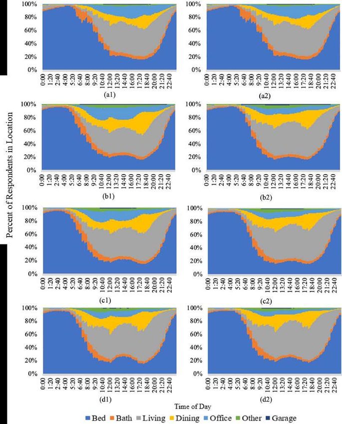
Figure 2. Spatial location of occupants (a) under 25; (b) 25–54; (c) 55–64; and (d) over 65, on (1)
weekdays and (2) weekends.......................................................................................................... 10
Figure 3. Hourly occupancy levels ............................................................................................... 11
Figure 4. Thermostat comfort set point comparisons ................................................................... 16
Figure 5. Weekday targeted fixture lighting profiles .................................................................... 24
Figure 6. Weekend targeted fixture lighting profiles .................................................................... 24
Figure 7. Vacation targeted fixture lighting profiles .................................................................... 25
Figure 8. Weekday targeted plug load profiles ............................................................................. 28
Figure 9. Weekend targeted plug load profiles ............................................................................. 28
Figure 10. Vacation targeted plug load profiles............................................................................ 29
Figure 11. Total energy savings for ENERGY STAR SHEMS in Boston ................................... 30
Figure 12. Total energy savings for ENERGY STAR SHEMS in Houston................................. 30
Figure 13. Total energy savings for ENERGY STAR SHEMS in Phoenix ................................. 31
Figure 14. HVAC energy savings for ENERGY STAR SHEMS ................................................ 32
Figure 15. Interior lighting energy savings for ENERGY STAR SHEMS .................................. 32
Figure 16. Plug load energy savings for ENERGY STAR SHEMS............................................. 33
List of Tables
Table 1. Matrix of Occupant Behavior With and Without HEMS Installed .................................. 5
Table 2. EnergyPlus Baseline Modeling Inputs .............................................................................. 6
Table 3. Key Literature Results Used in This Study ...................................................................... 7
Table 4. Weekday Occupancy Narrative ...................................................................................... 12
Table 5. Weekend Occupancy Narrative ...................................................................................... 13
Table 6. Assumed Demand Response Events for Modeling......................................................... 14
Table 7. Literature on Thermostat Settings, Based on Research by Pang et al. (2020) ................ 15
Table 8. Smart Thermostat Functions ........................................................................................... 17
Table 9. Weekday Thermostat Settings ........................................................................................ 20
Table 10. Weekend Thermostat Settings ...................................................................................... 21
Table 11. Vacation Thermostat Settings ....................................................................................... 22
Table 12. Connected Lighting Assumptions................................................................................. 23
Table 13. Targeted Light Fixture Operational Behavior Before and After HEMS Installation ... 23
Table 14. Targeted Plug Load Assumptions ................................................................................. 26
Table 15. Targeted Plug Load Operational Behavior ................................................................... 27
Table 16. Predicted Annual Energy Use for ENERGY STAR SHEMS ...................................... 34
viExecutive Summary
The objective of this study is to develop a repeatable and defensible methodology to analyze the
energy savings for home energy management systems (HEMS) that meets the minimum
requirements for certification under ENERGY STAR® Smart Home Energy Management System
(SHEMS) Version 1 (U.S. Environmental Protection Agency [EPA] 2020a). Mandatory
connected loads include a smart thermostat, two smart lights, and one smart power strip or smart
outlet. Control strategies must include feedback to occupants through an in-home display, user
programming, occupancy sensor-based controls, and responsiveness to utility signals such as
demand response programs.
Several occupant behavior patterns were selected to quantify the range of energy savings
potential for a HEMS with this basic functionality. A literature review was conducted to
establish realistic room-by-room occupancy levels and usage patterns for connected devices. A
series of event-driven hourly profiles were created, followed by adjustments based on application
of HEMS control strategies to thermostats, interior lighting, and plug load schedules.
EnergyPlus® modeling was performed using these hourly schedules in three locations (Boston,
Houston, and Phoenix) to examine climate dependence of energy savings.
Total site energy savings ranged from 4.3 to 27.1 MBtu/year (7%–35%), and utility bill savings
ranged from $123 to $670/year (6%–29%). The highest predicted savings was realized by
occupants that were not energy conscious prior to HEMS installation, but highly engaged with
the HEMS controls once the system was installed. The smart thermostat accounted for most of
the savings, followed by the smart power strip. Smart lighting did not save a significant amount
of energy in our analysis, based on an assumption that efficient LEDs with no standby power
would normally be installed anyway.
1 Introduction
Home energy management systems (HEMS) are part of a quickly expanding product market that
provides homeowners with the ability to control energy-consuming devices through monitoring
and feedback, programmed schedules, control logic based on occupancy sensors or weather data,
machine learning, and utility signals. The broad range of HEMS product combinations and the
high dependence on occupant behavior make it challenging to create modeling algorithms that
accurately estimate impacts on energy bills, especially under time-of-use rates. This inability to
quantify the benefits of HEMS has been identified by stakeholders as a major barrier to
qualifying HEMS for utility program incentives and energy efficiency credits in energy codes
(Hendron et al. 2020).
For this project, Frontier Energy leveraged previous work performed by the National Renewable
Energy Laboratory (NREL) in support of the Building America House Simulation Protocols
(HSP) (Wilson et al. 2014), along with more recent studies of energy savings for HEMS control
strategies conducted by Frontier and others, to simulate the range of expected energy and cost
1savings for a HEMS that minimally complies with the ENERGY STAR Smart Home Energy
Management System (SHEMS) Version 1 certification requirements (EPA 2020a). The
methodology developed under this project could increase demand for ENERGY STAR-certified
SHEMS by increasing consumer confidence in the likely range of energy savings for a basic
HEMS package. It is also an important step toward a flexible and repeatable method for
predicting the energy savings of any theoretical combination of HEMS capabilities, connected
devices, and occupant behavioral patterns.
1.1 ENERGY STAR Smart Home Energy Management System Requirements
The ENERGY STAR program finalized Version 1 of the SHEMS certification requirements in
September 2019 following extensive collaboration and review by HEMS manufacturers,
technology experts, and other stakeholders. Because we are focused on modeling systems that
comply with the minimum requirements of an ENERGY STAR-certified SHEMS, it is important
to identify which specific attributes are mandatory and which are optional. The relevant
requirements are summarized below:
• Connected End Uses
o Heating and cooling via ENERGY STAR Smart Thermostat (EPA 2017)
o Two smart lights (EPA 2020b) or fixtures (EPA 2019)
o One smart power strip/smart outlet
o Optional control of water heaters, appliances, batteries
• Control Methods
o Occupant feedback (energy use and recommended behavioral actions)
o User-established rules/schedules
o Occupancy sensor-based optimization
o Grid signals (demand response, possible load shifting)
o Optional use of predictive control and machine learning.
In most cases, the requirements related to connected devices and control strategies are very clear.
In other cases, EPA identifies general functionality that can be difficult to quantify in a building
energy model. The challenge for this project was to convert those requirements into specific
modifications to thermostat settings, heating, ventilating, and air-conditioning (HVAC)
availability, lighting and miscellaneous electric load (MEL) schedules and peak loads, and other
modeling inputs that may be affected by the operation of the HEMS.
2EPA has not published estimates of energy savings potential for SHEMS. Instead, the program
emphasizes the collection of field data for a range of compliant systems to demonstrate actual
savings in occupied homes. That information will be valuable in the long term, but it will likely
be two or three years before useful data are available. There is also the likelihood of new
technologies arriving on the market, making it challenging to obtain field test data before the
results become obsolete due to the rapid evolution and turnover of HEMS products.
1.2 Building America House Simulation Protocols
The 2014 update to the HSP, combined with the Building America Analysis Spreadsheets
(NREL 2011), provides much of the information needed to analyze HEMS in a consistent
manner. However, the HSP is primarily focused on disaggregation of detailed end uses, along
with standardized hourly and seasonal operating profiles. It does not provide guidance on how
controls would impact these profiles, nor does it provide discrete event-driven schedules for
individual devices or lamps. The HSP is also somewhat out of date, especially in the areas of
lighting and MELs where the market has evolved rapidly over the past 5–10 years. The HSP uses
constant thermostat settings of 71°F for heating and 76°F for cooling, which are based primarily
on occupant comfort according to ASHRAE Standard 55-2010 (ASHRAE 2010) and are not
necessarily realistic for most households. Finally, most schedules are the same on weekdays,
weekends, and vacation days, which is not as realistic as we would like for detailed HEMS
analysis.
32 Technical Approach
The first step for this project was a literature search to identify relevant work performed by other
researchers. This helped ensure that we built upon the best information available. Detailed
information about occupant behavior was sparse, but there have been several field studies
evaluating various common elements of HEMS functionality, especially related to smart
thermostats. There have also been a few modeling studies of the energy savings potential of
various types of control logic, most often related to predictive control and machine learning. In
addition, we investigated surveys of occupants regarding their attitudes toward HEMS and their
likelihood of overriding grid signals or preprogrammed controls. Further details on the literature
search are provided in Section 3.1.
Once we had a solid understanding of past work, we leveraged that knowledge to develop a
robust methodology for modeling the energy savings potential for an ENERGY STAR-certified
SHEMS. We focused on leveraging field studies that could provide direct modeling inputs, such
as studies of thermostat settings with and without a smart thermostat, or a specific fraction of
lights that are regularly turned off when rooms are unoccupied. In addition, we made use of
studies that provide energy savings for one technology, or a bundle of technologies, as a
calibration point for approximating reasonable behavioral changes that would result in
comparable energy savings in our model. If no field data were available to support specific
modeling inputs, we used engineering judgment to make reasonable assumptions about likely
operational changes following the installation of a HEMS with specific control logic.
The starting points for all operating conditions were those documented in the HSP and associated
spreadsheets. However, we needed to convert some of the smooth hourly profiles into more
realistic step functions based on specific devices turning on and off at certain times of day. We
also established specific occupancy levels in each room at each hour of the day, including
periods with nobody at home. This use of discrete behavioral patterns in relation to the operation
of specific devices was necessary to make realistic adjustments to loads based on HEMS
operation and grid signals.
Modeling inputs were developed for four combinations of behavior before and after HEMS
installation, as shown in Table 1. For the baseline cases without HEMS, the “Not Energy
Conscious” (NEC) case represents fairly high use occupants that generally don’t take actions to
minimize energy use, while “Very Energy Conscious” (VEC) occupants employ thermostat set-
back/set-up and usually attempt to turn off lights and electronic devices when not in use. In cases
with HEMS, the “Somewhat Engaged” household makes limited use of HEMS features and
sometimes overrides demand response signals. The “Highly Engaged” household uses all
features and does not override demand response or other signals except in unusual
circumstances, such as during a dinner party. There is also likely to be a group of “Not Engaged”
households that make no use of HEMS features. Though important, we did not model this case
4because the energy savings would be negligible or even negative due to HEMS standby losses.
Further details on the behavioral assumptions for each category are provided in Section 3.2.
Table 1. Matrix of Occupant Behavior With and Without HEMS Installed
Not Energy Conscious (NEC)
Without HEMS
Very Energy Conscious (VEC)
Somewhat Engaged (SE)
With HEMS
Highly Engaged (HE)
EnergyPlus was used for all modeling activity to allow maximum flexibility when implementing
the HEMS analysis methodology. The HSP requirements for new construction were used for all
uncontrolled end uses, along with the building envelope characteristics. A typical 2-story, 3-
bedroom, 2,150-ft2 single-family house geometry was selected for modeling, as shown in
Figure 1. Because discrete occupancy levels were required at all times for the purpose of
applying control logic, we assumed 3 occupants instead of the HSP default of 2.6. A summary of
baseline assumptions is provided in Table 2. Refinements to occupancy, thermostat, lighting, and
MEL schedules required for detailed modeling of HEMS are discussed in Section 3.2.
Figure 1. Representative house used for EnergyPlus modeling
5Table 2. EnergyPlus Baseline Modeling Inputs
House Characteristic Value
Floor area 2,150 ft2
Orientation East-facing
Number of stories 2
Number of bedrooms 3
Number of occupants 3
HVAC Gas furnace, air conditioner
Location Boston, Phoenix, Houston
Natural gas utility rate structure Fixed national average
Electric utility rate structure Representative time of use
Other house characteristics/schedules HSP default
Each of the four behavioral scenarios was modeled in three different cities (Boston, Houston, and
Phoenix) representing three different climate zones (cold, hot-humid, and hot-dry), resulting in
12 total modeling runs. The Boston model used a basement foundation, while Houston and
Phoenix used slab-on-grade. The three locations had differing heating and cooling seasons, latent
versus sensible cooling loads, lighting usage based on latitude, as well as systems interactions
between internal loads and HVAC energy.
Energy costs were calculated using a typical national time-of-use rate schedule developed by
Frontier Energy for another project (German and Hoeschele 2014), because some of the control
strategies were intended to shift load from more-expensive (4 to 9 p.m.) to less-expensive time
periods rather than simply to save energy. The peak cost from 4 to 9 p.m. year-round was
$0.30/kWh and the off-peak cost all other times was $0.10/kWh. A national average rate of
$1.0135/therm was used for natural gas as reported by the U.S. Energy Information
Administration (EIA) for 2019 (EIA 2021).
63 Project Results
The final results for this project include key findings from the literature search, the detailed
methodology used to adjust modeling inputs, and the range of energy savings calculated by the
EnergyPlus models.
3.1 Literature Search
The literature search revealed a range of experimental and theoretical studies that provided
valuable insights into the methodology that would be needed for this project. A summary of
literature search findings that we expected to use as part of the methodology, either as direct
modeling inputs, adjustments to baseline assumptions, or checks on energy savings calculations,
are summarized in Table 3. Further details about how these results were used are provided in
Section 3.2. Many additional publications were reviewed as part of the literature search but were
not explicitly used in the formulation of the HEMS analysis methodology, either because a more
appropriate reference was available or because the information was not aligned with our
technical approach. A more complete list and relevant summaries of these publications are
available upon request from the authors of this report.
Table 3. Key Literature Results Used in This Study
Category Attribute Value Source
Most common occupant age
Two people 25 to 34, one
combination for 3-person Mitra et al. (2020)
under 25
household
Occupancy
Daytime occupancy (at least 44% weekdays, 65%
Piper et al. (2017)
one person home) weekends
Room-by-room occupancy See Figure 2 Mitra et al. (2020)
Thermostat base comfort 76°F summer, Based on analysis of
settings 68°F winter Pang et al. (2020)
Daytime regular or temporary
5°F summer, Based on analysis of
vacancy setback/setup (when
9°F winter Pang et al. (2020)
used)
Thermostat
Nighttime setback/setup (when 5°F summer, Based on analysis of
used) 9°F winter Pang et al. (2020)
Demand response event
+3°F summer, Comparison with CEC
temperature offset (when
-3°F winter (2019)
used)
~30% of 2014 HSP
Household lighting energy Rubin et al. (2016)
lighting values
Living room lighting average 2.3 hrs/day (mix of
Rubin et al. (2016)
operating hours overhead/portable)
Lighting Bedroom lighting average 1.7 hrs/day (mix of
Rubin et al. (2016)
operating hours overhead/portable)
Living room percent portable 35% Rubin et al. (2016)
Bedroom percent portable 39% Rubin et al. (2016)
7Category Attribute Value Source
Lighting schedules on
Approximately the same Rubin et al. (2016)
weekday vs. weekend
Lighting that occurs with 25% of living room lighting, Urban, Roth, and Harbor
nobody present 35% of bedroom (2016)
Field study showing
increase in usage of 1
Smart lamp operating hours hr/day, but decrease in
Earle and Sparn (2019)
and dimming lumen-hours of 500 lm-
hrs/day, partially due to
dimming
50% installed in
Applied Energy Group
Smart lamp locations living/family room, 33% in
(2020)
bedrooms
54% lower duty cycle for
Urban, Roth, and Harbor
Occupancy sensor impact occupancy sensor vs.
(2016)
on/off controls
212 kWh/yr in 2017,
Potential whole-house lighting
efficiency based on older Piper et al. (2017)
savings
EIA study
Primary TV in active mode (not
7.7 hrs/day Rubin et al. (2016)
necessarily being watched)
Time average person watches Bureau of Labor Statistics
2.81 hrs/day
TV (2019)
Time average person plays 0.26 hrs/day (0.65 hrs/day Bureau of Labor Statistics
video games for 15–24 age range) (2019)
Background analysis for
Savings for Tier 2 Advanced
Wei et al. (2018) derived
Power Strip (APS) controlling 148 kWh/year
from Valmiki and
entertainment center
Corradini (2016)
Potential savings for Lamoureaux, Reeves,
8%
TVs/home entertainment and Hastings (2016)
MELs Potential primary TV savings 131 kWh/yr savings out of Urban, Roth, and Harbor
through circuit-level controls 274 kWh/yr (2016)
Background analysis for
APS standby power 1W
Wei et al. (2018)
TV standby power 1W Rubin et al. (2016)
TV active power 169 W Rubin et al. (2016)
Potential standby load
Lawrence Berkeley
reduction through optimal
30% National Laboratory
behavior with minimal
(2020)
inconvenience
Potential plug load savings for
341 kWh/yr with 15-minute
occupancy-based controls Piper et al. (2017)
time delay
(primarily home electronics)
8Category Attribute Value Source
260 kWh/yr (with HVAC),
Herter and Okuneva
In-home display savings ~219 kWh/yr (without
(2014)
HVAC)
In-home display savings
4%–7%, declines over
(feedback to occupants about Karlin et al. (2015)
time
energy use)
Lighting/plug load savings Not statistically significant, Applied Energy Group
impacts for demand response but consistently positive (2020)
Percent of devices turned back
Applied Energy Group
on during demand response 5%–20%
(2020)
events
Likelihood of further
Cross-
participation in demand Applied Energy Group
cutting 43%
response programs based on (2020)
experience with study
Demand response events in Southern California
14
2020 Edison (SCE) (2020)
Average number of demand 7.4 nationwide for Smart Electric Power
response events behavioral programs Alliance (2018)
4 W, not including
HEMS continuous power Earle and Sparn (2019)
thermostat
Savings for smart home 1760–2150 kWh/yr, 80
Kemper (2019)
bundle (all end uses) therms/yr
Savings for smart home 11% (net of 10% take-
Nadel and Ungar (2019)
bundle (all end uses) back effect)
9Percent of Respondents in Location
Figure 2. Spatial location of occupants (a) under 25; (b) 25–54; (c) 55–64; and (d) over 65, on (1) weekdays
and (2) weekends. (Mitra et al. 2020)
3.2 Analysis Methodology
The modifications made to the baseline EnergyPlus model to reflect the event-driven energy use
of HEMS-connected devices for each of the four categories of occupant behavior are described
in the following sections.
103.2.1 Occupancy
The occupancy profiles were developed by creating a narrative for the three occupants of the
house on weekdays and weekends, aligning occupancy as closely as possible with targeted
“typical” overall occupancy levels. The targeted hourly curves were created by adjusting the
HSP hourly profiles to better align with the Title 24 CASE Report on plug loads and lighting
(Rubin et al. 2016) for weekends and weekdays, while maintaining the same overall occupancy
levels for the week. The targeted total occupancy levels were 48 person-hours of occupancy on
weekdays, 54 person-hours of occupancy on weekends/holidays, and 0 person-hours during
vacation periods as defined in the HSP. Actual hourly occupancy levels (matching the targeted
total person-hours) used in the HEMS modeling are shown in Figure 3. These hourly occupancy
levels for modeling (dotted lines) were developed to provide more realism for the purpose of
HEMS modeling than the simple target occupancy levels, which were unrealistically smooth and
were expressed as fractions of people.
Figure 2. Hourly occupancy levels
Narratives for the three occupants on weekdays and weekends are shown in Table 4 and Table 5.
A legend indicating the room in the house where each activity takes place is included below each
table. Adult #1 works full time outside the home, while Adult #2 works part time. The Teenager
goes to school most of the day but does some schoolwork at home in the afternoon, perhaps
consistent with a freshman in college. The family has dinner together and sometimes participates
in family events together, such as going out to a movie. The rest of the time, family members
generally act independently.
These narratives are representative of the activities in which typical members of a household
would engage, and they are the same for all four types of energy use behavior. They were
carefully selected to align as closely as possible with data points from the literature documented
in Table 3. For example, the amount of time spent in the living room and the number of hours
watching TV are very comparable to the various field studies identified in the literature search.
With only a few day-types to choose from and only three occupants, this approach can only
11provide “representative” savings for HEMS under realistic conditions. To add a more realistic
range of behavioral patterns, the hours where nobody is home are clustered on weekdays, while
on weekends they are more dispersed. For a more comprehensive study of HEMS impacts, it
would be ideal to stochastically generate 365 days of activities, with probability distributions
based on field studies of occupant behavior, to better represent the range of behavior both within
a household over the course of a year, and across households throughout the United States.
Table 4. Weekday Occupancy Narrative
Hour Adult #1 Adult #2 Teenager
1
2
3
4 Sleep Sleep Sleep
5
6
7
8 Bathroom Breakfast Breakfast
9 Bathroom Bathroom
10 Work
11 Home for lunch
12 School
Work
13 Work
14
15
Cleaning Homework
16
17 Reading/TV Music
18 Dinner Dinner Dinner
19
Out to movies Out to movies Out to movies
20
21 Video games
Reading/TV
22 Reading/TV
TV
23 Computer
24 Sleep Sleep Sleep
Out of the House
Master Bedroom
Second Bedroom
Master Bathroom
Second Bathroom
Dining Room
Living Room
Office
12Table 5. Weekend Occupancy Narrative
Hour Adult #1 Adult #2 Teenager
1
2
3
4 Sleep Sleep Sleep
5
6
7
8 Breakfast Breakfast Breakfast
9 Bathroom Cleaning Video games
10 Yardwork
Yardwork Yardwork
11 TV
12 TV Bathroom Music
13 Lunch/errand Shopping
14 Reading Cleaning Friends/soccer
15 Soccer practice Soccer practice
16 Nap Homework
Reading
17 Long walk Shopping
18 Dinner Dinner
Dinner/dishes
19 Pay bills Video games
20 Shopping Music
TV/video games
21 Reading TV
22 Ice cream shop Ice cream shop Ice cream shop
23 TV Reading TV
24 Sleep Sleep Sleep
Out of the House
Master Bedroom
Second Bedroom
Master Bathroom
Second Bathroom
Dining Room
Living Room
Office
3.2.2 Demand Response Events
Representative demand response events were derived from the 2020 SCE signals for the Smart
Energy Program (SCE 2020). The 14 events from SCE occurred primarily on the hottest days
and were often clustered together during a heat wave. We used Typical Meteorological Year
(TMY) 3 data to select the hottest 14 days for each of the three sites we modeled. SCE event start
times and durations were rounded off to the nearest hour, and were applied in sequence to the 14
13TMY3 days, as shown in Table 6. This is a simplification of the true range of demand response
events that occur under different programs for different electric utilities around the United States,
which may have cold weather events and morning events. A more comprehensive analysis of
demand response programs and drivers of specific demand response events would be valuable as
a future research topic.
Table 6. Assumed Demand Response Events for Modeling
Event # Start Time End Time
1 7 p.m. 8 p.m.
2 5 p.m. 9 p.m.
3 7 p.m. 8 p.m.
4 7 p.m. 8 p.m.
5 7 p.m. 8 p.m.
6 6 p.m. 8 p.m.
7 7 p.m. 8 p.m.
8 5 p.m. 9 p.m.
9 3 p.m. 7 p.m.
10 6 p.m. 8 p.m.
11 3 p.m. 7 p.m.
12 2 p.m. 6 p.m.
13 5 p.m. 8 p.m.
14 4 p.m. 8 p.m.
3.2.3 Thermostat
Thermostat settings vary quite a bit throughout a single day, across different day types, and for
the different behavioral scenarios. To describe how temperature settings were selected for this
study, temperature set points used or recommended by various sources are presented in Table 7
based upon research by Pang et al. (2020).
14Table 7. Literature on Thermostat Settings, Based on Research by Pang et al. (2020)
Heating Cooling
Reference Setpoint Setpoint Note
(Setback) (Setback)
ENERGY STAR® 78°F Recommendation
Building America House
Simulation Protocol (Wilson et 71°F 76°F Recommendation
al. 2014)
ASHRAE Standard 55
68.5°–75°F 75°–80.5°F Recommendation
(ASHRAE comfort zones)
2018 International Energy
Conservation Code (IECC)
(International Code Council 72°F 75°F Recommendation
[ICC] 2018) (manual
thermostat)
2018 IECC (ICC 2018)
≤72°F ≥78°F Recommendation
(programmable thermostat)
Analysis of literature review,
Florida Solar Energy Center
67°F 77°F measurements, and Residential
(FSEC) (2013)
Energy Consumption Survey
Analysis of 327 North American
Booten et al. (2017) 70°F 75°F
home thermostat measurements
Huchuk, O'Brien, and Sanner Analysis of 10,250 North America
70°F 75°F
(2018) home thermostat measurements
Pang et al. (2020) (“little
70°F (0) 75°F (0) Assumption, based on past studies
environmental awareness”)
Pang et al. (2020) (“acceptable
70°F (-7) 75°F (+7) Assumption, based on past studies
environmental awareness”)
Pang et al. (2020) (“good
70°F (-15) 75°F (+15) Assumption, based on past studies
environmental awareness”)
Pang et al. (2020) (“excellent
66°F (-11) 79°F (+11) Assumption, based on past studies
environmental awareness”)
The settings used in those studies are illustrated in Figure 4, along with the assumed comfort
preferences that were selected to be used in this study (“NREL”).
1580 Legend
Assumed comfort preferences
79 7 NREL used in this study (described
COOLING SETPOINT (°F)
below)
78 3 6 Booten et al. (2017); Huchuk et
al. (2018); and Pang et al. (2020)
1
77 4
(little, acceptable, and good
awareness)
76 NREL 2 2 Building America
3 ENERGY STAR
75 1 5 4 FSEC (2013)
5 IECC (manual)
74
64 66 68 70 72 74 6 IECC (programmable)
HEATING SETPOINT (°F) Pang et al. (2020) (excellent
7
awareness)
Figure 3. Thermostat comfort set point comparisons
Most of the set points used in these other studies are aspirational rather than reflecting actual
behavior. For example, Meier et al. (2011) found in a survey that almost 90% of respondents
indicated that they rarely or never set a schedule on their programmable thermostat. Pritoni et al.
(2015) reviewed case studies of the energy savings realized by programmable thermostats and
found that only a third provided savings compared with manual thermostats, and some even
increased energy use. Most of the set points from the other studies are also either
recommendations or averages.
In the present study, comfort preferences were assumed to be 68°F in winter and 76°F in
summer—close to the averages of the setpoints in these studies. The intent in this study was to
provide set points that reflect a range of behavioral scenarios; however, all the settings assumed
are based upon the same assumed actual comfort preferences (the temperature at which an
occupant is assumed to find the best balance between comfort and energy costs). So, the base
comfort preference settings of 68°F and 76°F were adjusted for each of the different behavior
scenarios and throughout the day for different day types.
Smart thermostats affect the effective temperature set point at any given time in many different
ways, which vary by make and model, and are often not well documented. Table 8 shows some
of the functions that smart thermostats tend to use to minimize HVAC energy use or shift peak
demand while maintaining comfort. These functions were analyzed to consider how they would
affect the temperature set points throughout the day and combined to develop an assumed
effective thermostat set point schedule for modeling the impact of the smart thermostat and what
a thermostat schedule would look like if these functions were not used.
16Table 8. Smart Thermostat Functions
Occupant Feedback Improved Algorithms
• Metrics and Reports Predictive Control and Machine Learning
• Interactive Charts • Learning Schedules
• Data Download • Learning Temperatures
User-Established Rules/Schedules • Optimum Start
• Error-Free Schedules • Compressor Optimization
• Flexible Schedules • Real-Feel Temperature
• Recommended Schedules Improved Interfaces for Operation
Occupancy Sensor-Based Optimization • System Mode
• Vacancy Detection • Accidental Permanent Holds
• Averaging Temperatures • Vacation Holds
Grid Signals • Temporary Holds
• Time of Use Optimization • Efficient Default with Override
• Demand Response Event Response • Comfort Default with Override
The assumptions that were used in developing the assumed schedules were as follows:
Not Energy Conscious (NEC):
• Comfort Setting: The thermostat settings were 72°F for heating and 72°F for cooling.
This does not accurately reflect the base comfort preferences due to misprogramming.
This is a worst-case assumption, but one that is probably a reality for many homes that
are not paying any attention to energy conservation.
• Setback: The homeowners do not adjust their thermostats for nighttime setbacks, or when
leaving the home for brief absences or vacations.
Very Energy Conscious (VEC):
• Comfort Setting: Again, the misprogrammed settings may not reflect true preferences for
comfort, so the occupied period set point was 69°F for heating and 75°F for cooling.
• Setback: There is a 9°F setback for heating, and a 5°F setback for cooling at night and
during vacation periods. There is no setback for either regular vacancies during the day or
brief absences.
• Optimal Start: There is no optimal start function for the thermostat, so that the occupant
sets the thermostat to begin an hour prior to waking or returning home (this is a
simplification, and it may be more or less than an hour in a real home).
• Schedule: The thermostat time periods are not correctly set, so that the system starts an
additional hour earlier in the morning and prior to returning home, and it runs an hour
longer than necessary after going to bed or leaving for the day.
• Note: There are many very energy-conscious occupants who faithfully use their
thermostats as “on/off” switches, and manually adjust their setpoints optimally
throughout the day. These occupants can experience the lowest energy use, even without
17sophisticated controls. However, they also run the potential to forget to make changes
and waste energy. While this behavior is not uncommon, it was not used as the definition
of a Very Energy Conscious occupant for the purposes of this study.
Somewhat Engaged (SE):
• Comfort Setting: The settings are a closer reflection of true preferences for comfort, so
the occupied period set point was 68°F for heating and 76°F for cooling.
• Setback: There is a 9°F setback for heating, and 5°F for cooling during nighttime, regular
daytime vacancies, periodic unexpected absences, and vacations. However, the
occupancy sensors only detect about half of the unexpected vacancies.
• Optimal Start: There is an optimal start function for the thermostat, so the heating or
cooling system begins immediately upon waking or returning home. (Note that in reality,
the system would not begin immediately when the comfort period begins. This
simplifying assumption had to be made, because subhourly temperature adjustments are
not possible using an hourly simulation model. A preheating or precooling period of more
or less than an hour could be expected, but it is assumed to be shorter in this scenario
than in the previous one).
• Schedule: The thermostat time periods are a closer reflection of actual daily schedules,
but still not perfect. The system starts an hour earlier in the morning and prior to
returning home, and it runs an hour longer than necessary after going to bed or leaving
for the day.
Highly Engaged (HE):
• Comfort Setting: The settings reflect an attempt by the homeowner to be very energy
conscious and to set the temperature a bit beyond their base comfort preference. They are
able to do this because they can very readily override the temperature anytime they find
themselves uncomfortable. We assume that the setting is two degrees warmer in summer
and cooler in winter for most occupied hours, but that for one or two hours a day they
override this setting and set the thermostat temporarily at their base comfort preference.
• Setback: There is a 9°F setback for heating, and a 5°F setback for cooling during
nighttime, regular daytime vacancies, all periodic unexpected absences, and vacations.
• Optimal Start: There is an optimal start function for the thermostat, so the heating or
cooling system begins immediately upon waking or returning home. (Note again that sub-
hourly temperature adjustments are not possible using an hourly simulation model, so this
is a simplification, and in reality, a preheating or precooling period of less than an hour
would be expected).
18• Schedule: The thermostat time periods are an exact reflection of actual daily schedules,
due to learning algorithms and vacancy detection.
• Demand Response: Any time a demand response event is called (using the demand
response event schedule described elsewhere), the thermostat set point is adjusted by 3°F,
regardless of time of day, day type, occupancy, or vacation status. The resulting set points
vary, but for occupied hours, tend to be 63°F for heating and 81°F for cooling. For
comparison, Title 24 requires an occupant controlled smart thermostat to have a default
demand response set point in cooling mode of 82°F, and heating mode 60°F (CEC,
2019).
There were no adjustments to thermostat settings based on geographic location. Heating and
cooling seasons were established based on the HSP default.
The resulting adjusted set points that were used in this study are shown in Table 9 through
Table 11. For these schedules, the home’s occupancy matches that assumed for the other end
uses (VACANT indicates that ALL occupants are absent, and OCCUPIED indicates that ANY
occupant is present). In any scenarios where the temperature setting was not optimally tracking
the actual activities of the occupants (for reasons described below), the temperature is
highlighted. Occupant energy consciousness level (NEC, VEC) and level of smart thermostat
engagement (SE, HE) are the same as defined in Table 1.
19Table 9. Weekday Thermostat Settings (Nonoptimal settings are highlighted)
Heating Cooling
Actual Thermostat
HOUR
NEC
NEC
VEC
VEC
Activity Assumptions
HE
HE
SE
SE
0–1 Sleep Sleep 72 60 59 57 72 80 81 83
1–2 Sleep Sleep 72 60 59 57 72 80 81 83
2–3 Sleep Sleep 72 60 59 57 72 80 81 83
3–4 Sleep Sleep 72 60 59 57 72 80 81 83
4–5 Sleep Sleep 72 60 59 57 72 80 81 83
5–6 Sleep Pre-heating/cooling? 72 69 59 57 72 75 81 83
6–7 Sleep Starts too early? 72 69 68 57 72 75 76 83
7–8 Occupied Occupied 72 69 68 66 72 75 76 78
8–9 Occupied Occupied 72 69 68 66 72 75 76 78
9–10 Vacant Missed vacancy? 72 69 59 57 72 75 81 83
10–11 Occupied Occupied 72 69 68 66 72 75 76 78
11–12 Vacant Missed vacancy? 72 69 59 57 72 75 81 83
12–13 Vacant Missed vacancy? 72 69 59 57 72 75 81 83
13–14 Vacant Starts too early? 72 69 68 57 72 75 76 83
14–15 Occupied Occupied 72 69 68 66 72 75 76 78
15–16 Occupied Occupied 72 69 68 66 72 75 76 78
16–17 Occupied Extra comfort? 72 69 68 68 72 75 76 76
17–18 Occupied Occupied 72 69 68 66 72 75 76 78
18–19 Vacant Missed vacancy? 72 69 59 57 72 75 81 83
19–20 Vacant Missed vacancy? 72 69 68 57 72 75 76 83
20–21 Occupied Occupied 72 69 68 66 72 75 76 78
21–22 Occupied Occupied 72 69 68 66 72 75 76 78
22–23 Occupied Occupied 72 69 68 66 72 75 76 78
23–24 Sleep Runs too long? 72 69 68 57 72 75 76 83
20Table 10. Weekend Thermostat Settings (Nonoptimal settings are highlighted)
Heating Cooling
Actual Thermostat
Hour
NEC
NEC
VEC
VEC
Activity Assumptions
HE
HE
SE
SE
0–1 Sleep Sleep 72 60 59 57 72 80 81 83
1–2 Sleep Sleep 72 60 59 57 72 80 81 83
2–3 Sleep Sleep 72 60 59 57 72 80 81 83
3–4 Sleep Sleep 72 60 59 57 72 80 81 83
4–5 Sleep Sleep 72 60 59 57 72 80 81 83
5–6 Sleep Pre-heating/cooling? 72 69 59 57 72 75 81 83
6–7 Sleep Starts too early? 72 69 68 57 72 75 76 83
7–8 Occupied Occupied 72 69 68 66 72 75 76 78
8–9 Occupied Occupied 72 69 68 66 72 75 76 78
9–10 Vacant Missed vacancy? 72 69 59 57 72 75 81 83
10–11 Occupied Occupied 72 69 68 66 72 75 76 78
11–12 Occupied Occupied 72 69 68 66 72 75 76 78
12–13 Vacant Missed vacancy? 72 69 59 57 72 75 81 83
13–14 Occupied Occupied 72 69 68 66 72 75 76 78
14–15 Vacant Missed vacancy? 72 69 59 57 72 75 81 83
15–16 Occupied Occupied 72 69 68 66 72 75 76 78
16–17 Occupied Occupied 72 69 68 66 72 75 76 78
17–18 Occupied Occupied 72 69 68 66 72 75 76 78
18–19 Vacant Extra comfort? 72 69 68 68 72 75 76 76
19–20 Vacant Extra comfort? 72 69 68 68 72 75 76 76
20–21 Occupied Occupied 72 69 68 66 72 75 76 78
21–22 Vacant Missed vacancy? 72 69 68 57 72 75 76 83
22–23 Occupied Occupied 72 69 68 66 72 75 76 78
23–24 Sleep Runs too long? 72 69 68 57 72 75 76 83
21Table 11. Vacation Thermostat Settings (Nonoptimal settings are highlighted)
Heating Cooling
Actual Thermostat
Hour
NEC
NEC
VEC
VEC
Activity Setting
HE
HE
SE
SE
0–1 Vacant Missed vacancy? 72 60 59 57 72 80 81 83
1–2 Vacant Missed vacancy? 72 60 59 57 72 80 81 83
2–3 Vacant Missed vacancy? 72 60 59 57 72 80 81 83
3–4 Vacant Missed vacancy? 72 60 59 57 72 80 81 83
4–5 Vacant Missed vacancy? 72 60 59 57 72 80 81 83
5–6 Vacant Missed vacancy? 72 60 59 57 72 80 81 83
6–7 Vacant Missed vacancy? 72 60 59 57 72 80 81 83
7–8 Vacant Missed vacancy? 72 60 59 57 72 80 81 83
8–9 Vacant Missed vacancy? 72 60 59 57 72 80 81 83
9–10 Vacant Missed vacancy? 72 60 59 57 72 80 81 83
10–11 Vacant Missed vacancy? 72 60 59 57 72 80 81 83
11–12 Vacant Missed vacancy? 72 60 59 57 72 80 81 83
12–13 Vacant Missed vacancy? 72 60 59 57 72 80 81 83
13–14 Vacant Missed vacancy? 72 60 59 57 72 80 81 83
14–15 Vacant Missed vacancy? 72 60 59 57 72 80 81 83
15–16 Vacant Missed vacancy? 72 60 59 57 72 80 81 83
16–17 Vacant Missed vacancy? 72 60 59 57 72 80 81 83
17–18 Vacant Missed vacancy? 72 60 59 57 72 80 81 83
18–19 Vacant Missed vacancy? 72 60 59 57 72 80 81 83
19–20 Vacant Missed vacancy? 72 60 59 57 72 80 81 83
20–21 Vacant Missed vacancy? 72 60 59 57 72 80 81 83
21–22 Vacant Missed vacancy? 72 60 59 57 72 80 81 83
22–23 Vacant Missed vacancy? 72 60 59 57 72 80 81 83
23–24 Vacant Missed vacancy? 72 60 59 57 72 80 81 83
3.2.4 Smart Lighting
To meet SHEMS certification requirements, two ENERGY STAR-certified smart lamps or smart
fixtures must be controlled. The rooms most likely to include smart lamps and fixtures are living
rooms and bedrooms (Applied Energy Group, 2020). Our assumption is that the overhead
fixtures in the living room and master bedroom are connected to the HEMS. In most homes,
these fixtures will have LED lamps with manual on/off controls and no dimming capability.
Smart fixtures connected to a HEMS are assumed to have a small continuous standby power,
dimming capability, and programmable timing for security purposes. Additional characteristics
of the assumed light fixtures and controls are summarized in Table 12, along with the reference
or other basis for the assumption.
22Table 12. Connected Lighting Assumptions
Lighting Attribute Without HEMS With HEMS Basis
Fixture type Overhead Overhead Judgment
Lamp type LED LED Judgment
Living Room (LR): 4,
Number of lamps LR: 4, BR: 2 EPA (2021)
Bedroom (BR): 2
Based on Rubin et al.
Hours of useful light 3 3
(2016)
Fixture power LR: 12 W, BR: 6 W LR: 12 W, BR: 6 W EPA (2021)
Standby power 0W LR: 1 W, BR: 0.5 W EPA (2019)
Dimmed power N/A LR: 6 W, BR: 3 W Judgment
Occupancy, dimming,
Controls On/off voice activation, EPA (2020a)
demand response
Assumed operation of connected lighting in the living room and bedroom varies for each of the
four categories of energy use behavior, as shown in Table 13. Key differences include how often
and for how long lights are left on after leaving the room, use of dimming capability, frequency
of overrides, enrollment in demand response programs, and use of programmed scheduling.
Table 13. Targeted Light Fixture Operational Behavior Before and After HEMS Installation
Behavioral Without HEMS With HEMS
Basis
Attribute
NEC VEC SE HE
1 hour after Occupancy No Judgment based
Lights on in 1-2 hours after
occupancy, sensor occupancy on Urban, Roth,
unoccupied occupancy,
1/3 of the override 1/2 sensor and Harbor
rooms 2/3 of the time
time of the time overrides (2016)
2 hrs/day
Always on in
Vacation Always off Always off on in LR, Judgment
LR, off in BR
off in BR
Not Used 1/3 of Used 2/3 of
Dimming Not available Judgment
available the time the time
Demand Not Applied Energy
Not available Not enabled Always off
response available Group (2020)
Application of these behavioral patterns to the connected lighting features in Table 12 and the
occupancy schedules defined in Section 3.2.1 resulted in the hourly connected lighting energy
profiles shown in Figure 5, Figure 6, and Figure 7, for weekdays, weekends, and vacation
periods respectively.
2320
18
16
14
Power (W)
12
10
8
6
4
2
0
1 2 3 4 5 6 7 8 9 10 11 12 13 14 15 16 17 18 19 20 21 22 23 24
Hour of Day
VEC NEC SE HE
Figure 5. Weekday targeted fixture lighting profiles
20
18
16
14
Power (W)
12
10
8
6
4
2
0
1 2 3 4 5 6 7 8 9 10 11 12 13 14 15 16 17 18 19 20 21 22 23 24
Hour of Day
VEC NEC SE HE
Figure 4. Weekend targeted fixture lighting profiles
2414
12
10
Power (W) 8
6
4
2
0
1 2 3 4 5 6 7 8 9 10 11 12 13 14 15 16 17 18 19 20 21 22 23 24
Hour of Day
VEC NEC SE HE
Figure 7. Vacation targeted fixture lighting profiles
To create the lighting curves for the EnergyPlus models, the total lighting energy in the HSP was
first reduced by 70% based on the Title 24 CASE report (Rubin et al. 2016). Next, the connected
component of the lighting energy (expressed as smooth hourly curves) in the Building America
Analysis Spreadsheet (NREL 2011) was subtracted from the national average total lighting
curves for October (approximately consistent with the annual average) and replaced with the
event-driven lighting schedules in Figure 5, Figure 6, and Figure 7. Additional profiles were
created for the 14 demand response event days, where connected lights were assumed to be
turned off during peak demand periods. The monthly multipliers and latitude-specific multipliers
in the Building America Analysis Spreadsheet were then applied to the hourly curves, which
were then imported into the models to provide realistic annual lighting energy savings estimates
for the smart lighting component of the HEMS.
3.2.5 Advanced Power Strip
ENERGY STAR SHEMS requires one connected smart power strip or smart outlet. For this
analysis, we selected a Tier 2 APS controlling the primary entertainment system, including a TV,
set-top box, and video game system. Other potential components of the entertainment system are
assumed to be connected to uncontrolled outlets. The APS was assumed to have sensors that
detect both occupancy and infrared signals from remote controls. It was also assumed that the
APS was controlled through voice activation, programmed using the HEMS interface, and
disabled in response to grid signals during demand response events. A summary of the attributes
of connected plug loads is provided in Table 14, along with the reference or other basis for the
assumption.
25Table 14. Targeted Plug Load Assumptions
Lighting Attribute Without HEMS With HEMS Basis
Entertainment center:
Valmiki and Corradini
Connected devices N/A primary TV, set-top box,
(2016)
video game system
Connected load N/A 200 W NREL (2011)
APS standby power N/A 1W Wei et al. (2018)
169 W active, 169 W active, 1 W standby,
TV power Rubin et al. (2016)
1 W standby 0 W off
Bureau of Labor Statistics
TV hours of active 4 hrs/day weekday, 4 hrs/day weekday,
(2019) and Rubin et al.
use 6 hrs/day weekend 6 hrs/day weekend
(2016)
21 W active, 21 W active, 16 W standby,
Set-top box power NREL (2011)
16 W standby 0 W off
4 hrs/day weekday,
Set-top box hours of 4 hrs/day weekday,
4 hrs/day weekend, Judgment based on
active use or DVR 4 hrs/day weekend,
2 hours/day NREL (2011)
recording 2 hours/day vacation
vacation
Video game system 10 W active, 10 W active, 2 W standby,
NREL (2011)
power 2 W standby 0 W off
Video game system 1 hr/day weekday, 1 hr/day weekday, Bureau of Labor Statistics
hours of active use 2 hrs/day weekend 2 hrs/day weekend (2019)
APS location N/A Living room Judgment
Occupancy, remote control
On/off
Controls sensor, voice activation, EPA (2020a)
(active/standby)
demand response
Use of the entertainment system controlled by the APS varies based on the category of
operational behavior with and without the APS and HEMS, as described in Table 15. Key
differences include how often and for how long devices are left on when no longer in use,
whether devices are put in standby mode versus being turned off completely, frequency of APS
overrides, and engagement in demand response programs.
26Table 15. Targeted Plug Load Operational Behavior
Without HEMS With HEMS
Behavioral
Basis
Attribute
NEC VEC SE HE
Off when Off when
TV and video
1 hour after 1 hour after unoccupied unoccupied
game system Judgment based on
occupancy, occupancy, and not in and not in
left on in Valmiki and
2/3 of the 1/3 of the use, APS use, no
unoccupied Corradini (2016)
time time override 1/2 APS
rooms after use
of the time overrides
Set-top box left Left on Off when
Programmed
on in Left on 24 during the unoccupied
to turn off at Judgment
unoccupied hrs/day day, off at and not in
night
rooms night use
TV and
video game All devices All devices
TV and
system in off except off except
video game
standby, set-top box set-top box
system in
set-top box on for on for
Vacation standby, set- Judgment
on for scheduled scheduled
top box left
scheduled DVR DVR
on 24
DVR recording recording
hrs/day
recording only only
only
Off,
Judgment based on
Demand Not including
Not available Not enabled Applied Energy
response available DVR
Group (2020)
recording
Hourly profiles were developed for weekday, weekend, and vacation days after applying these
behavioral patterns to the occupancy narratives described in Section 3.2.1 and connected plug
load characteristics in Table 14. These profiles are illustrated in Figure 8, Figure 9, and Figure
10.
27250
200
Power (W)
150
100
50
0
1 2 3 4 5 6 7 8 9 10 11 12 13 14 15 16 17 18 19 20 21 22 23 24
Hour of Day
VEC NEC SE HE
Figure 8. Weekday targeted plug load profiles
250
200
Power (W)
150
100
50
0
1 2 3 4 5 6 7 8 9 10 11 12 13 14 15 16 17 18 19 20 21 22 23 24
Hour of Day
VEC NEC SE HE
Figure 9. Weekend targeted plug load profiles
2825
20
Power (W)
15
10
5
0
1 2 3 4 5 6 7 8 9 10 11 12 13 14 15 16 17 18 19 20 21 22 23 24
Hour of Day
VEC NEC SE HE
Figure 10. Vacation targeted plug load profiles
Inputs for the EnergyPlus models were developed by removing the standard HSP connected
devices from the hourly curves for MELs using the Detailed MEL Analysis Worksheet tab in the
Building America Analysis Spreadsheet for New Construction (NREL 2011). The discrete
electricity use patterns for the connected devices were then added back in, and new hourly curves
were created for the three day-types (weekday, weekend/holiday, vacation) along with 14
demand response days. Seasonal adjustments were overlaid on these curves using the monthly
Home Entertainment multiplier under the Monthly Profiles tab. No adjustments were made to the
plug load curves based on geographic location.
3.3 Modeling Results
The total energy and cost savings predictions for the HEMS in each of the three climates and for
each of the four combinations of pre- and post-installation occupant behavior are shown in
Figure 11, Figure 12, and Figure 13. Since the non-HEMS occupant behavior scenarios
essentially “bracket” the range of expected non-HEMS behaviors, and there is no data on where
the average home lies within this range, it is reasonable to look at the average of the two non-
HEMS scenarios. Similarly, because the HEMS occupant behavior scenarios essentially
“bracket” the range of expected HEMS behaviors, and there is very limited data that can shed
light on where the average home lies within this range, it is reasonable to look at the average of
the two HEMS scenarios. Therefore, the average savings of the four comparisons is a reasonable
estimate of expected savings for our purposes.
Average site energy savings for gas and electricity ranged from 19.7% to 22.1%, and cost
savings ranged from 16.2% to 17.9%. Although the savings vary by location, especially the split
between gas and electric, it is noteworthy that total site energy savings is fairly consistent for the
three locations we selected. The HEMS control strategies we modeled do not seem to take full
advantage of the time of use rate schedules. Much of the electricity savings occurs at night and
29You can also read