Modeling of Border Irrigation in Soils with the Presence of a Shallow Water Table. I: The Advance Phase - MDPI

Page created by Eva Mcdonald
 
CONTINUE READING
Modeling of Border Irrigation in Soils with the Presence of a Shallow Water Table. I: The Advance Phase - MDPI
agriculture

Article
Modeling of Border Irrigation in Soils with the Presence of a
Shallow Water Table. I: The Advance Phase
Sebastián Fuentes               and Carlos Chávez *

                                          Water Research Center, Department of Irrigation and Drainage Engineering, Autonomous University
                                          of Queretaro, Cerro de Las Campanas SN, Col. Las Campanas, Queretaro 76010, Mexico;
                                          sebastian.fuentes@uaq.mx
                                          * Correspondence: chagcarlos@uaq.mx; Tel.: +52-442-192-1200 (ext. 6036)

                                          Abstract: The overelevation of the water table in surface irrigation plots is one of the main factors
                                          affecting salinization in agricultural soils. Therefore, it is necessary to develop simulation models
                                          that consider the effect of a shallow water table in the process of advance-infiltration of the water in
                                          an irrigation event. This paper, the first in a series of three, develops a simple mathematical model
                                          for the advance phase of border irrigation in soils with the presence of a shallow water table. In
                                          this study, the hydrodynamic model of the Barré de Saint-Venant equations is used for the water
                                          surface flow, and the equations are solved using a Lagrangian finite-differences scheme, while in the
                                          subsurface flow, an analytical solution for infiltration in soils with a shallow water table is found
                                          using the bisection method to search for roots. In addition, a hydraulic resistance law is used that
                                          eliminates the numerical instabilities presented by the Manning–Strickler law. The model results
                                          for difference irrigation tests show adjustments with an R2 > 0.98 for the cases presented. It is also
                                          revealed that, when increasing the time step, the precision is maintained, and it is possible to reduce
                                          the computation time by up to 99.45%. Finally, the model proposed here is recommended for studying
                                the advance process during surface irrigation in soils with shallow water tables.
         
Citation: Fuentes, S.; Chávez, C.
                                          Keywords: Barré de Saint-Venant equations; hydrodynamic model; analytical solution; flow profiles;
Modeling of Border Irrigation in Soils
                                          irrigation tests; inverse modeling; water use efficiency; agricultural water management
with the Presence of a Shallow Water
Table. I: The Advance Phase.
Agriculture 2022, 12, 426. https://
doi.org/10.3390/agriculture12030426
                                          1. Introduction
Academic Editors: Yanqun Zhang
                                               Surface irrigation is one of the main factors in the fluctuation of shallow water tables in
and Jiandong Wang
                                          agricultural plots. Around the world, surface irrigation is the most frequently used method
Received: 5 March 2022                    for water application in agricultural plots, where the water is distributed over the field and
Accepted: 17 March 2022                   through the soil [1].
Published: 18 March 2022                       The presence of a shallow water table changes the water content of the soil profile
                                          (Figure 1), due principally to the capillary process, which is present in porous media [2]. It
Publisher’s Note: MDPI stays neutral
with regard to jurisdictional claims in
                                          has been found that in shallow water conditions, irrigation can be reduced by up to 80%
published maps and institutional affil-
                                          without affecting yield and without increasing soil salinity [3].
iations.                                       Poor design of surface irrigation, for example losses from tailwater due to the selection
                                          of an inappropriate irrigation flow or due to poor operation in the water distribution
                                          network as a result of poor leveling in the ground by percolation, can cause overelevation
                                          of the water table and the progressive salinization of the soil [4].
Copyright: © 2022 by the authors.              It is estimated that 20% of the arable land and 33% of irrigated agricultural plots
Licensee MDPI, Basel, Switzerland.        in the world are affected by high salinity [5]. Water-table levels play an essential role in
This article is an open access article    the salt distribution in the soil profile and could be controlled by subsurface drainage [6].
distributed under the terms and           However, drainage leads to an increase in irrigation costs. Therefore, it is necessary to
conditions of the Creative Commons        model surface irrigation both for the surface water movement and infiltration into the soil,
Attribution (CC BY) license (https://     using an equation that considers soil with a shallow water table for the latter.
creativecommons.org/licenses/by/
4.0/).

Agriculture 2022, 12, 426. https://doi.org/10.3390/agriculture12030426                                  https://www.mdpi.com/journal/agriculture
Modeling of Border Irrigation in Soils with the Presence of a Shallow Water Table. I: The Advance Phase - MDPI
Agriculture 2022,
  Agriculture     12, 12,
               2022,  x FOR
                          426 PEER REVIEW                                                                                                        2 of 212
                                                                                                                                                        of 12

                                      Figure
                                   Figure     1. Irrigation
                                          1. Irrigation     scheme
                                                         scheme    in soils
                                                                in soils    with
                                                                         with    shallow
                                                                              shallow    water
                                                                                       water    table.
                                                                                             table.

                                           The border irrigation water flow can be characterized using the hydrodynamic model
                                        The border irrigation water flow can be characterized using the hydrodynamic model
                                      of the Barré de Saint-Venant equations, which accurately describes surface irrigation [7].
                                   of the Barré de Saint-Venant equations, which accurately describes surface irrigation [7].
                                      The relationship between the width and the water depth in a border makes it possible
                                   The relationship between the width and the water depth in a border makes it possible to
                                      to consider the equations corresponding to runoff for an infinite surface width [8]. The
                                   consider the equations corresponding to runoff for an infinite surface width [8]. The con-
                                      continuity equation in the hydrodynamic model is written as follows:
                                   tinuity equation in the hydrodynamic model is written as follows:
                                                                                    ∂h ∂q ∂I
                                                                                        h ∂q+ ∂I = 0
                                                                                       ∂+                                                                 (1)
                                                                                    ∂t +∂x +∂t = 0                                                    (1)
                                                                                       ∂t ∂x ∂t
                                      and the momentum equation is as follows [9]:
                                   and the momentum equation is as follows [9]:

                                                             2 ∂q         ∂q+ gh33 − q22 ∂∂h                                    ∂I ∂I = 0
                                                           2 ∂q          ∂q                
                                                                                   (              )
                                                                                                h + gh      3
                                                         hh     ++2hq
                                                             ∂t∂t 2hq∂x       + gh − q          ∂x+ gh 3 ( J(−J −
                                                                                                                J o J)o+) β+qhβqh   =0                (2)(2)
                                                                          ∂x                   ∂x                               ∂t ∂t
                                      where
                                   where      q(x,t)
                                           q(x,t)      = U(x,t)h(x,t)
                                                   = U(x,t)h(x,t)  is theis discharge
                                                                            the discharge       per width
                                                                                         per unit      unit width
                                                                                                               of theof       the border
                                                                                                                           border           or the unitary
                                                                                                                                     or the unitary dis-
                                      discharge,    x is the  spatial  coordinate     in the    main    direction      of
                                   charge, x is the spatial coordinate in the main direction of the water movement in the   the water    movement    in the
                                      border,   t is the  time,   U is  the  mean     velocity,   h   is  the water        depth,
                                   border, t is the time, U is the mean velocity, h is the water depth, VI =I ∂I(x,t)/∂t is the     V   = ∂I(x,t)/∂t is the
                                      infiltration flow, that is, the water volume infiltrated per unit width per unit length of the
                                   infiltration flow, that is, the water volume infiltrated per unit width per unit length of the
                                      border, I is the infiltrated depth, g is gravitational acceleration, β = U /U is a dimensionless
                                   border, I is the infiltrated depth, g is gravitational acceleration, β = UIX                   IX/U is a dimension-
                                      parameter where UIX is the projection in the direction of the output velocity of the water
                                   less parameter where UIX is the projection in the direction of the output velocity of the
                                      mass due to the infiltration, Jo is the topographic slope, and J is the friction slope that can
                                   water mass due to the infiltration,          Jo is the topographic slope, and J is the friction slope
                                      be determined by the fractal law of hydraulic resistance [10]:
                                   that can be determined by the fractal law of hydraulic resistance [10]:
                                                                                                         !d
                                                                                                 3 3 Jg
                                                                                                         d
                                                                                                h
                                                                                                h Jg   
                                                                                     q=
                                                                                     q = kkν
                                                                                           ν  ν 2 2 
                                                                                                                                                   (3) (3)
                                                                                               ν 
                                      where
                                   where          is the
                                           ν isν the      kinematic
                                                      kinematic     viscosity
                                                                 viscosity    coefficient,
                                                                            coefficient, k isk aisdimensionless
                                                                                                   a dimensionless    factor
                                                                                                                   factor thatthat includes
                                                                                                                                includes   thethe
                                   effects of soil roughness, and the exponent d has a fractal interpretation. From this law,the
                                      effects  of  soil roughness,  and the  exponent   d has    a fractal interpretation.  From    this law,
                                   theChezy
                                       Chezyformula
                                                formulaisisdeduced
                                                              deducedwith
                                                                       withdd==1/21/2 and
                                                                                      and the
                                                                                           the Poiseuille
                                                                                                  Poiseuille law
                                                                                                              law with
                                                                                                                  with dd == 1.
                                                                                                                             1.
                                         TheThe    initial
                                               initial  andand boundary
                                                             boundary      conditions
                                                                        conditions   forfor  a closed
                                                                                         a closed       border,
                                                                                                      border,     avoiding
                                                                                                                avoiding     loss
                                                                                                                          loss  byby   tailwater
                                                                                                                                    tailwater
                                      outside   the   irrigation domain,  are as
                                   outside the irrigation domain, are as follows: follows:

                                                                                   q(qx,( 0x,0
                                                                                            ) =) =0 0; ;hh(x,
                                                                                                           ( x,0
                                                                                                              0) )== 00                              (4)(4)

                                                                          q (t0,t
                                                                        q(0,  ) =) =
                                                                                   q0q; q; (qx(fx, t),t=
                                                                                       0           f   ) =00; ; hh((xxf ,f ,tt))== 00
                                                                                                                              (5)(5)
                                     where xf (t) is the position of the wave front at time t and qo is the unitary discharge at the
                                   where xf (t) is
                                     entrance   ofthe
                                                   theposition
                                                      border. of the wave front at time t and qo is the unitary discharge at the
                                   entrance of the border.
Agriculture 2022, 12, 426                                                                                                                                            3 of 12

Agriculture 2022, 12, x FOR PEER REVIEW                                                                                                                            3 of 12

                                          Numerous practical situations require a numerical solution of the Richards equation,
                                 with dimensions depending on the complexity of the studied problem. In surface irrigation,
                                 a one-dimensional
                                          Numerous practical      equation       is sufficient
                                                                          situations         requiretoa numerical
                                                                                                            represent the           infiltration
                                                                                                                              solution             phenomenon
                                                                                                                                          of the Richards             [11].
                                                                                                                                                              equation,
                                 However,         the   equation      lacks    general        analytical      solutions,
                                 with dimensions depending on the complexity of the studied problem. In surface irriga-        and    therefore   complex     numerical
                                 methods
                                 tion,           are often required
                                           a one-dimensional                    in order
                                                                         equation                to solve it
                                                                                            is sufficient       to [12–14].
                                                                                                                     representThere        are other physics-based
                                                                                                                                     the infiltration     phenomenon
                                 [11]. However, the equation lacks general analytical solutions, andin
                                 models       resulting        from    the  simplification             of  the   initial    conditions,          particular
                                                                                                                                              therefore       the Green
                                                                                                                                                           complex    nu-
                                 and Ampt
                                 merical            equation
                                              methods          are[15].
                                                                    oftenThis     equation
                                                                             required               has been
                                                                                              in order              useditin[12–14].
                                                                                                             to solve            surfaceThere
                                                                                                                                            irrigation   [16–18].
                                                                                                                                                   are other        How-
                                                                                                                                                                physics-
                                 ever, with
                                 based      models  thisresulting
                                                            equation,from onlythe a homogeneous
                                                                                       simplificationmoisture    of the initialprofile    can be represented
                                                                                                                                      conditions,     in particular in the
                                                                                                                                                                       the
                                 soil   profile.
                                 Green and Ampt equation [15]. This equation has been used in surface irrigation [16–18].
                                 However, Fuentes with et al.
                                                            this[19]  developed
                                                                  equation,      onlyan        analytical solution
                                                                                            a homogeneous                    of theprofile
                                                                                                                       moisture        Richardscanequation     using the
                                                                                                                                                     be represented      in
                                 Green      and
                                 the soil profile.  Ampt      hypotheses       to  describe         the   infiltration      of  water    into  the  soil with  a shallow
                                 water table
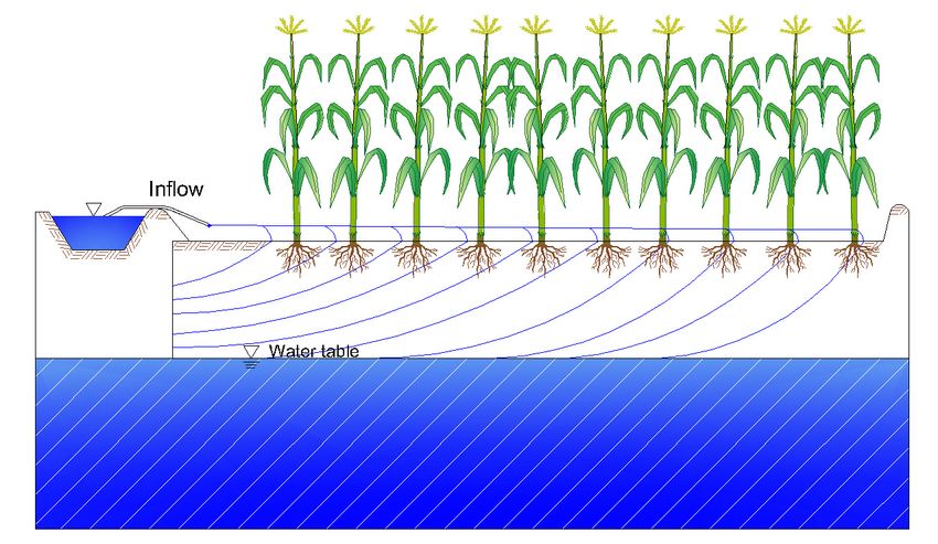
                                 Fuentes       et al.(Pf ).[19]
                                                             Thedeveloped
                                                                   solution considers
                                                                                  an analytical   a hydrostatic
                                                                                                           solutioninitialof the  moisture
                                                                                                                                     Richards  distribution   (Figurethe
                                                                                                                                                  equation using         2),
                                 where       the    initial    moisture       is  calculated          with
                                 Green and Ampt hypotheses to describe the infiltration of wateri into the     the    expression        θ (z)  = θ   +  (θ  −  θ  )(z/P
                                                                                                                                                   o soils witho a shal-  f ).
                                 Thus,
                                 low        the moisture
                                        water      table (Pf).content        at the soil
                                                                   The solution                 surfacea is
                                                                                        considers                θi (0) = θo initial
                                                                                                             hydrostatic         and atmoisture
                                                                                                                                          the water-table      surface is
                                                                                                                                                       distribution
                                 (Figure 2), where the initial moisture is calculated with the expression θi(z) = θo + (θs at
                                 θ i (P f ) = θ s .  The     suction    in the    wetting         front    is a  linear     function     of  the  moisture    content      −
                                 the
                                 θ     front, hf (θi ,θ
                                   o)(z/Pf). Thus,
                                                              s) =
                                                            the     hf (θs −content
                                                                 moisture        θi )/(θs −          o ), soil
                                                                                               at θthe    thatsurface
                                                                                                                 is:         is θi(0) = θo and at the water-table
                                 surface is θi(Pf) = θs. The suction in the wetting front                                is a linear
                                                                                                                                  zf
                                                                                                                                      function of the moisture
                                 content at the front, hf (θi,θsh) f=[θhi f(z(θf )s,−θsθ]i)/(θ       = hsf −(θθoo,),θsthat   −
                                                                                                                       ) 1 is:                                          (6)
                                                                                                                                  Pf
                                                                                                                                      zf 
                                 such that hf [θi (0),θs ] = hf and hfh              [θf i(P  ( z ) , θ  =The
                                                                                             θi ),θ
                                                                                               f fs ] = s0.
                                                                                                                 h f (infiltrated
                                                                                                                       θo , θs )  1 − depth
                                                                                                                                          
                                                                                                                                       Pf  is defined by:
                                                                                                                                                                        (6)
                                                                                                                                 
                                 such that hf[θi(0),θs] = hf and hf[θi(Pf),θs]zZf=(t)0. The infiltrated depth is defined by:
                                                                                                     z (t)
                                                                                                     s − θ (z)]dz
                                                                                                   f
                                                                                    I(t) =        [θ                                                                    (7)
                                                                                         I ( t ) =  θs −i θi ( z )  dz                                             (7)
                                                                                                 0    0
                                 that
                                 that is:
                                      is:
                                                                                                                     1 1
                                                               ( t )=I1M −= 1[1−−1z−f (zt)f /P
                                                                                              ( t )f ]P2 ,f IM, =IM2 =∆θP
                                                                                                               2
                                                        I(t)/IIM                                                          ΔθPf
                                                                                                                         2 f
                                                                                                                                                                        (8)
                                 where
                                 where IIM is the maximum infiltrated depth.
                                         M is the maximum infiltrated depth.

                                 Figure 2. Soil
                                           Soil moisture
                                                moisture profile with a shallow water table.

                                     Introducing Equation (6) into the Green and Ampt equation yields the differential
                                 equation for the analytical solution that considers a shallow water table [19]:
                                                                  h + h f ( 1 − z f Pf ) 
                                                       dI
                                                           = K s 1 +                      , z f = Pf 1 − 1 − I I M (9)        (                    )
                                                       dt                  zf           
Agriculture 2022, 12, 426                                                                                                4 of 12

                                Introducing Equation (6) into the Green and Ampt equation yields the differential
                            equation for the analytical solution that considers a shallow water table [19]:

                                                          h + hf (1 − zf /Pf )
                                                                              
                                            dI                                               p         
                                               = Ks 1 +                          , zf = Pf 1 − 1 − I/IM       (9)
                                            dt                     zf

                                 When the water depth is independent of time, h = h, and integration of Equation (9)
                            with the condition I = 0 at t = 0 leads to the following infiltration equation, where hf 6= Pf :
                                                              
                                                                   Pf          2 Pf (h+Pf )(h+hf )IM
                                                                      hf I −
                                                              
                                                               Pf −
                                                              
                                                                                           hf ) 3
                                                                                     (Pf −q
                                                              
                                                              
                                                               h                                    i
                                                                           P f − hf               I
                                                      Ks t =     ln 1 +              1 − 1 − IM                        (10)
                                                                           h+hf
                                                                   2 Pf (h+hf )IM
                                                                                          q         
                                                                                                    I
                                                              
                                                               +
                                                              
                                                                               2      1 − 1 − IM
                                                                       (Pf −hf )

                            and when hf = Pf :                      "                      #
                                                                                  I 3/2 2
                                                                                   
                                                              Pf IM   I   2
                                                      Ks t =            +     1−       −                                   (11)
                                                             h + Pf IM    3      IM      3

                            where h ∼ = [4d/(5d + 1)]ho is the mean water depth and ho = (ν2 /gJo )1/3 (qo /kν)1/3d is the
                            normal depth [20].
                                  Equation (10) reduces to the Green and Ampt infiltration equation when Pf → ∞,
                            considering that IM = 1/2∆θPf . In this limit, 1 – (1 – I/IM )1/2 ∼ = I/2IM = I/∆θPf holds. The
                            third term is of the order of 1/Pf and tends to zero. In the second term, the argument of the
                            logarithm tends to 1 + I/∆θ(h + hf ) and its coefficient to ∆θ(h + hf ). Finally, in the first term,
                            the coefficient of I → 1. Using the definition λ = ∆θ (h + hf ), the Green and Ampt equation
                            is deduced.
                                  In recent years, many different software packages have been developed to model
                            surface irrigation (e.g., [21,22]); however, they have some limitations due to the infiltration
                            equations used. For example, they only represent constant initial moisture conditions along
                            a homogeneous soil column, and they are empirical equations for a specific irrigation event.
                            Furthermore, they are not representative for the soils with shallow water tables (where the
                            moisture profile is not constant) existing in some irrigated agricultural areas.
                                  The objectives of this study, the first in a series of three, are: (a) to model the advance
                            phase of surface irrigation in a soil with a shallow water table by coupling an analytical
                            solution to the Barré de Saint-Venant equations and (b) to validate the model obtained with
                            data from an irrigation test reported in the literature. In the second paper, the three phases
                            of irrigation will be included: advance, storage, and recession. Finally, in the third article,
                            this solution will be compared with the Barré de Saint-Venant equations coupled internally
                            with the Richards equation.

                            2. Materials and Methods
                            Numerical Solution
                                The numerical solution of the Barré de Saint-Venant equations uses a Lagrangian
                            scheme [9,23]. The discrete form of the continuity equation is as follows:
                                             h                  i
                                               ωqL + (1 − ω)qJ δt − [ωqR + (1 − ω)qM ]δt
                                               −[ϕhL + (1 − ϕ)hR + ϕIL + (1 − ϕ)IR ](xR − xL )
                                               +[ω(hR + IR ) + (1 − ω)(hM + IM )](xR − xM )                                (12)
                                               −[ω(hL + IL ) + (1 − ω)(hJ + IJ )](xL − xJ )
                                               +[ϕhJ + (1 − ϕ)hM + ϕIJ + (1 − ϕ)IM ](xM − xJ ) = Rc

                                 Due to the numerical instability presented in the calculation cells at the beginning,
                            a discrete form of the momentum equation was developed, considering the following
Agriculture 2022, 12, 426                                                                                                                       5 of 12

Agriculture 2022, 12, x FOR PEER REVIEW                                                                                                        5 of 12
                                 assumptions: (a) the derivatives in time were calculated as a rectangular cell (Eulerian)
                                 and (b) average flow and water depth coefficients were considered for the calculation of an
                                 average friction slope. The discrete form of the momentum equation is as follows:
                                                                                   (           )
                                                  2hq ω ( q R − q L ) + ( 1 − ω) q M − q J  δt
                                                                                            i 
                                                    (            )                            (           )
                                             h                                 
                                                                     1 (−h ω−) hqM
                                                                                 L)
                                        2hq ω(+qRgh    −3q−L )q +2 
                                                                   (ω                + ( 1 −J ω)δth M − h J  δt
                                                                                       −  q
                                            3                           R                                
                                        + gh −
                                            2
                                                        {
                                                     q2 2  [ω(hR − hL ) + (1 − ω)(hM − hJ )]δt
                                                                                                                     (
                                              n + h ϕq L + ( 1 − ϕ ) q R  ( xR − xLh) − ϕq J + ( 1 − ϕ ) qiM  xM − x Jo    )}                 (13)
                                                                                                                                                  (13)
                                                            (1 − ϕ)q ](x − x ) − ϕq + (1 − ϕ)q (x − xJ )
                                        +h [ϕqL +
                                              3
                                                                                               (          )
                                                  +gh 3( J − J o ) ωR( x R R− x L ) L+ ( 1 − ω) JxM − x J  δt M M
                                                                                                           
                                        +gh J − Jo [ω(xR − xL ) + (1 − ω)(xM − xJ )]δt
                                                            {                                                            (       )}
                                                  +λδtqh ϕI L + ( 1 − ϕ ) I R  ( xR − xL ) − ϕI J + ( 1 − ϕ ) I M  xM − x J = Rm
                                        +λδtqh{[ϕIL + (1 −           ϕ)IR ](xR − xL ) − [ϕIJ + (1 − ϕ)IM ](xM − xJ )} = Rm
                                 where Rc and Rm represent the residuals of the continuity equation and momentum, re-
                                 spectively,
                                 where   Rc and theRm      representq the
                                                    coefficient           = ω[(1    − φ)qRof+ the
                                                                              residuals          φqLcontinuity
                                                                                                     ] + (1 − ω)[(1  − φ)qM and
                                                                                                                  equation    + φqmomentum,
                                                                                                                                   J], and the coef- re-
                                 spectively,   the  coefficient      q  =  ω[(1   −    ϕ)q     + ϕq    ] + (1 −   ω)[(1  −
                                 ficient h = ω[(1 − φ)hR + φhL] + (1 − ω)[(1 − φ)hM + φhJ], taking into account the extreme
                                                                                             R       L                     ϕ)q  M +   ϕq J ], and   the
                                 coefficient h = ω[(1 − ϕ)hR + ϕhL ] + (1 − ω)[(1 − ϕ)hM + ϕhJ ], taking 2into account                          the ex-
                                 values of each calculation cell, and consequently the coefficient J = ν ( q /kν)1/d/g h 3 . The                      3
                                 treme                                                                                            2           1/d
                                 weightvalues
                                          factors offor
                                                     each timecalculation
                                                                  and space  cell,
                                                                                areand     consequently
                                                                                       denoted    ω and φ,the    coefficient J = ν (q/kν) /gh .
                                                                                                              respectively.
                                 The weight     factors for
                                       In the discrete          timeaand
                                                             forms,          spacefactor
                                                                         weight        are denoted
                                                                                              in spaceωofandφ =ϕ,  respectively.
                                                                                                                 1/2 was considered for interior
                                       In the discrete forms, a weight factor in space of ϕ = 1/2 was considered for interior
                                 cells [23–26]. For the last cell and the first time step, φ = π/4 was used, deduced from the
                                 cells [23–26]. For the last cell and the first time step, ϕ = π/4 was used, deduced from the
                                 analysis of the short-time coupling of the Saint-Venant and Richards equations [27]. The
                                 analysis of the short-time coupling of the Saint-Venant and Richards equations [27]. The
                                 weight factor for time was taken as ω = 0.60 [24–26,28].
                                 weight factor for time was taken as ω = 0.60 [24–26,28].
                                       Figure 3 shows the Lagrangian cells during the advance phase. The subscripts L and
                                       Figure 3 shows the Lagrangian cells during the advance phase. The subscripts L and
                                 R denote the values of each variable to the left and right of the next time ti+1, and J and M
                                 R denote the values of each variable to the left and right of the next time ti+1 , and J and M
                                 represent the values at the current time ti.
                                 represent the values at the current time ti .

                                 Figure 3. Computational grid for the advance phase.
                                                                              phase.

                                       The
                                        The solution
                                            solution developed
                                                      developed is is implicit,   where Equations
                                                                      implicit, where     Equations (12)
                                                                                                      (12) and
                                                                                                           and (13)
                                                                                                                (13) are
                                                                                                                      are solved
                                                                                                                          solved simul-
                                                                                                                                  simul-
                                 taneously
                                 taneously for all cells at each time step. By linearizing the discrete equations, a system of
                                             for all cells at each time  step.   By linearizing   the discrete equations,   a system   of
                                 2N
                                 2N ++ 22 nonlinear
                                          nonlinear algebraic
                                                      algebraicequation
                                                                 equationwith
                                                                            with2N 2N+ +4 4unknown
                                                                                            unknownvariables    is is
                                                                                                        variables  produced,
                                                                                                                      produced,where
                                                                                                                                  whereN
                                 is
                                 N the   number
                                    is the number ofof
                                                     computational
                                                       computational   cells.
                                                                         cells.The
                                                                                Thesolution
                                                                                     solutionofofthe
                                                                                                  thesystem
                                                                                                      systemisisobtained
                                                                                                                 obtained byby applying
                                                                                                                               applying
                                 the
                                 the double sweep algorithm, which assumes a linear relation between the variation of
                                      double  sweep   algorithm,   which   assumes    a linear relation  between    the variation  of the
                                                                                                                                      the
                                 water   depth δh  and   the discharge  δq  in  a given  time step
                                 water depth δh and the discharge δq in a given time step [29]:     [29]:

                                                                              δqi = δEqi+i 1=δh
                                                                                              E ii++δh + F
                                                                                                   1 Fii+1 i +1                                   (14)
                                 and for the last cell the equation is expressed in terms of the advance distance, considering
                                 that δhN and δqN are equal to zero:
                                                                                            δδ = FN +1                                            (15)
Agriculture 2022, 12, 426                                                                                                    6 of 12

                               and for the last cell the equation is expressed in terms of the advance distance, considering
                               that δhN and δqN are equal to zero:

                                                                              δδ = FN+1                                         (15)

                               where the values of E and F are calculated by the partial derivatives of the residual equations
                               of continuity and momentum for each cell with respect to hL , qL , hR , and qR .
                                    With the coefficient values E and F, the improved solution for the new values of flow,
                               water depth, and position of the wave front is determined by:

                                                                    hni +1 = hni + δhi , 0 ≤ i ≤ N                              (16)

                                                                    qni +1 = qni + δqi , 1 ≤ i ≤ N                              (17)

                                                                          δxnN+1 = δxnN + δδ                                    (18)
                                    The convergence criterion selected for advancing in time is that the residual values
                               of the continuity equation (Rc) and the momentum equation (Rm) in the current iteration
                               must be less than 1 × 10⁻⁵ .
                                    The analytical solution for infiltration in a soil with a shallow water table is obtained
                               using the bisection method, which is widely used to find the roots of a function.

                               3. Results
                               3.1. Soil Characterization
                                    Simulations were performed with the information reported by Pacheco [30] for a
                               clay soil from La Chontalpa, Tabasco, Mexico, using the coupling of the Barré de Saint-
                               Venant equations and the analytical solution to model infiltration in a soil with a shallow
                               water table. The measured data from the irrigation tests were: border width B = 10.5 m,
                               border length L = 100 m, border slope Jo = 0.00085 m/m, moisture content at saturation
                               θs = 0.5245 cm3 /cm3 , and the dimensionless parameter β = 0. The values of the hydraulic
                               conductivity at saturation (Ks ) and the suction in the wetting front (hf ) were optimized using
                               the Levenberg–Marquardt algorithm [31]. In the hydraulic resistance law, Equation (3),
                               d = 1 was used. The values of qo , Pf , IM , initial moisture (θo ), h, Ks , and hf are reported in
                               Table 1 for each irrigation test.

                               Table 1. Values of the initial conditions in three irrigation tests.

    Test        qo (m3 /s/m)   Pf (cm)     IM (cm)       θo (cm3 /cm3 )        h (cm)        Ks (cm/h)   hf (cm)        R2
     1            0.001428      152          14.54           0.3331             2.73           1.1800     23.84        0.9983
     2            0.001428      50           2.15            0.4386             2.73           1.5325     44.00        0.9814
     3            0.001238      52           2.32            0.4353             2.60           0.0500     10.00        0.9967

                                    This table shows the correlation coefficient R2 between the measured data and those
                               calculated with the optimized parameters of Ks and hf . Good adjustments were observed
                               for the three irrigation tests.

                               3.2. Applications
                                    Simulations corresponding to each irrigation test were performed using the values
                               reported in Table 1 and the optimized values of Ks and hf .
                                    Figure 4 shows the good fit of the measured data for the advance phase and those
                               obtained by the proposed model when optimizing the values of Ks and hf , which is
                               corroborated by the high R2 values obtained.
Agriculture 2022, 12, x FOR PEER REVIEW                                                                                          7 of 12
Agriculture
Agriculture2022,
            2022,12,
                  12,x426
                        FOR PEER REVIEW                                                                                          7 7ofof12
                                                                                                                                         12

                                         100
                                         100
                                          90
                                          90
                                          80
                                          80
                                          70
                                          70

                                         (min)
                                          60
                                       (min)
                                          60
                                    Time  50
                                          50
                                          40
                                  Time

                                          40
                                          30
                                          30                                                             Pf = 152 cm
                                          20
                                                                                                         Pf = 152 cm
                                                                                                              50 cm
                                          20
                                          10                                                             Pf = 50
                                                                                                              52 cm
                                          10                                                             Pf = 52 cm
                                           0
                                           0 0          20          40          60             80             100      120
                                             0          20          40          60
                                                                           Distance (m)        80             100      120
                                                                          Distance (m)
                                 Figure 4. Evolution of the advance front in the border irrigation with shallow water table.
                                             Evolutionof
                                  Figure4.4.Evolution
                                 Figure                ofthe
                                                          theadvance
                                                              advancefront
                                                                      frontin
                                                                            inthe
                                                                               theborder
                                                                                  borderirrigation
                                                                                         irrigation with
                                                                                                    with shallow
                                                                                                         shallow water
                                                                                                                 water table.
                                                                                                                        table.
                                  3.3.
                                   3.3. Comparison
                                        Comparisonofofthe
                                                        the Theorical
                                                            Theorical Advance
                                                                       Advance Curve
                                                                                 Curve with
                                                                                        with the
                                                                                              the Measured
                                                                                                   Measured Data
                                                                                                             Data
                                 3.3. Comparison
                                         The        of the
                                             information   Theorical
                                                            from   theAdvance
                                                                       second   Curve  with
                                                                                irrigation  the
                                                                                           test   Measured
                                                                                                  (P         Data
                                                                                                    f = 50 cm) was used for a more ex-
                                         The information from the second irrigation test (Pf = 50 cm) was used for a more
                                        The information
                                  haustive   analysis.      from
                                                        Figure    the second
                                                                5 shows        irrigation
                                                                          the advance      test obtained
                                                                                         curve    (Pf = 50 cm)
                                                                                                            by was  used for
                                                                                                               the by
                                                                                                                   model,    a more
                                                                                                                           which    ex-
                                                                                                                                 shows
                                   exhaustive    analysis.   Figure  5 shows    the advance      curve obtained       the model,  which
                                 haustive
                                    good afitanalysis.
                                  ashows       between  Figure
                                                          the   5 shows
                                                              measured    the advance
                                                                           data  obtainedcurve
                                                                                           in    obtained
                                                                                                the  field  by
                                                                                                           and the model,
                                                                                                               those       which
                                                                                                                      obtained
                                             good fit between the measured data obtained in the field and those obtained with    shows
                                                                                                                               with the
                                 amodel.
                                    good   fit
                                   the model.  between   the  measured    data   obtained  in  the   field and those  obtained with the
                                 model.
                                                 70
                                                 70
                                                 60
                                                 60
                                                 50
                                                 50
                                         (min)

                                                 40
                                       (min)

                                                 40
                                    Time

                                                 30
                                  Time

                                                 30
                                                 20
                                                 20
                                                 10                                              Measured data
                                                 10                                              Model development
                                                                                                 Measured data
                                                  0                                              Model development
                                                  0 0    20              40           60                 80            100
                                                    0    20              40Distance (m)
                                                                                      60                 80            100
                                                                          Distance (m)
                                  Figure 5.
                                 Figure     Evolutionof
                                         5. Evolution ofthe
                                                         theadvance
                                                             advance front
                                                                      front in
                                                                             in the
                                                                                 the second
                                                                                     second irrigation
                                                                                             irrigation test.
                                                                                                        test.
                                 Figure 5. Evolution of the advance front in the second irrigation test.
                                        Figure 6 shows that when the infiltrated depth reaches the I calculated with Equation (8),
                                        Figure 6 shows that when the infiltrated depth reaches M        the IM calculated with Equa-
                                  the soil
                                       Figureis noshows
                                                    longerthat
                                                             capable ofthe
                                                                         storing   more water.reaches
                                                                                                 Therefore,
                                                                                                        the IMthe soil was with
                                                                                                                             considered
                                 tion (8),  the 6soil           when
                                                      is no longer capable  infiltrated
                                                                             of storing depth
                                                                                        more water. Therefore,  calculated       Equa-
                                                                                                                   the soil was consid-
                                  completely
                                 tion  (8), the  saturated
                                                soil  is no  36 min
                                                            longer  after
                                                                   capable irrigation
                                                                             of storinghad started.
                                                                                        more  water.  Therefore,   the soil was consid-
                                 ered completely saturated 36 min after irrigation had started.
                                        The surfacesaturated
                                 ered completely         and subsurface    flowirrigation
                                                                 36 min after     profiles are
                                                                                           hadshown
                                                                                                started.in Figure 7, where it can be
                                  observed that the infiltration over all points of the border is limited by the maximum
                                  infiltration shown in Figure 6. It is also evident from the third curve (39 min), that a
                                  determined region of the soil was already at saturation, because the soil could no longer
                                  store more water. Due to the complexity of obtaining the roots in the analytical solution,
                                  the time used for this process was 55 min; however, the time discretization can be increased
                                  to obtain reliable results in a shorter time.
Cumulative infiltration (cm
                                                                                                        2.00

                                                                                                        1.50
Agriculture
 Agriculture2022, 12,12,
              2022,   x FOR
                         426 PEER REVIEW                                                                                                                              8 of8 of
                                                                                                                                                                            1212

                                                                                                        1.00

                                                                                                  2.50
                                                                                                   0.50

                                                Cumulative infiltration (cm)
                                                                                                  2.00
                                                                                                   0.00
                                                                                                               0        10           20          30         40
                                                                                                  1.50                              Time (min)
                                   Figure 6. Evolution of the infiltrated depth in a border irrigation with a shallow water table.
                                       1.00
                                         The surface and subsurface flow profiles are shown in Figure 7, where it can be ob-
                                   served
                                        0.50that the infiltration over all points of the border is limited by the maximum infil-
                                   tration shown in Figure 6. It is also evident from the third curve (39 min), that a deter-
                                   mined region of the soil was already at saturation, because the soil could no longer store
                                        0.00
                                   more water. Due to the complexity of obtaining the roots in the analytical solution, the
                                              0               10            20             30             40
                                   time used for this process was 55 min; however, the time discretization can be increased
                                                                           Time (min)
                                   to obtain reliable results in a shorter time.
                                    Figure
                                  Figure 6. 6. Evolution
                                            Evolution  ofof the
                                                          the   infiltrated
                                                              infiltrated   depth
                                                                          depth inin a border
                                                                                   a border   irrigationwith
                                                                                            irrigation   witha ashallow
                                                                                                                  shallowwater
                                                                                                                          watertable.
                                                                                                                                 table.

                                         4 surface and subsurface flow profiles are shown in Figure 7, where it can be ob-
                                        The
                                  served that the infiltration over all points of the border is limited by the maximum infil-
                                            Water depth (cm)

                                  tration shown in Figure 6. It is also evident from the third curve (39 min), that a deter-
                                         3
                                  mined region of the soil was already at saturation, because the soil could no longer store
                                  more water. Due to the complexity of obtaining the roots in the analytical solution, the
                                  time used
                                         2   for this process was 55 min; however, the time discretization can be increased
                                  to obtain reliable results in a shorter time.

                                                                                            1
                                                                                           4
                                                 (cm) (cm)

                                                                                                          0        20        40           60          80     100
                                                                                            1
                                                depth

                                                                                           3
                                           depth

                                                                                                                                                           13.0 min
                                    Infiltrated

                                                                                            2                                                              26.0 min
                                                                                           2
                                                                                                                                                           39.0 min
                                    Water

                                                                                                                                                           51.9 min
                                                                                            3
                                                                                           1                                      Distance (m)
                                    Infiltrated depth (cm)

                                    Figure 7. Flow profiles every 13 min of a border irrigation with a shallow water table.
                                   Figure 7. Flow profiles every 13 min of a border irrigation with a shallow water table.
                                           0           20            40           60             80           100
                                    3.4.1Time Step Analysis
                                   3.4. Time
                                         An Step Analysis
                                             analysis of the computation time was performed at different values of δt in the
                                         An analysis   of the  computation   time was performed   atand13.0 minvalues of δt in the
                                                                                                     different
                                    numerical    coupling  of the  Barré de Saint-Venant  equations      the analytical solution of
                                        2                                                              26.0
                                   numerical
                                    infiltrationcoupling  of the Barré
                                                  with a shallow        detable.
                                                                    water  Saint-Venant
                                                                                 Table 2 equations and
                                                                                          shows that    the min
                                                                                                      there  analytical
                                                                                                             was        solution for
                                                                                                                  no difference   of
                                   infiltration
                                    the differentwith a shallow
                                                    values  of δt water table.
                                                                  studied      Table
                                                                           here. The2 computer    there39.0
                                                                                                        wasmin
                                                                                       shows thatequipment    no difference
                                                                                                              used          for the
                                                                                                                    to perform   the
                                   different  values            ® CoreTM i7-4710                       51.9tomin
                                    simulations
                                        3         hasof
                                                      anδtIntel
                                                           studied   here. The computer
                                                                                  CPU @ equipment
                                                                                         2.50 GHz andused
                                                                                                        32 Gbperform
                                                                                                               of RAM.the simula-
                                   tions has an Intel Core i7-4710 Distance
                                                      ®       TM         CPU @ 2.50(m)GHz and 32 Gb of RAM.
                                         Table 2. Computation time for different time steps (δt).
                                  Figure 7. Flow profiles every 13 min of a border irrigation with a shallow water table.2
                                                   δt                    Computation Time (min)                       R
                                                  1.0
                                  3.4. Time Step Analysis                        55.0
                                                   1.5                           14.5                           1.0
                                        An analysis2.0
                                                      of the computation time was 8.2
                                                                                     performed at different values
                                                                                                                1.0
                                                                                                                    of δt in the
                                  numerical coupling
                                                   5.0   of the Barré de Saint-Venant
                                                                                  1.3  equations and the analytical
                                                                                                                1.0 solution of
                                  infiltration with  a shallow water table. Table 0.3
                                                  10.0                            2 shows that there was no difference
                                                                                                                1.0      for the
                                  different values of δt studied here. The computer equipment used to perform the simula-
                                  tions has an Intel® CoreTM i7-4710 CPU @ 2.50 GHz and 32 Gb of RAM.
δt           δt                  Computation  Time Time
                                                                                                                                         Computation   (min) (min)                       R        R2
                                                                                                    1.0          1.0                          55.0 55.0
                                                                                                    1.5          1.5                          14.5 14.5                                1.0        1.0
                                                                                                    2.0          2.0                           8.2 8.2                                 1.0        1.0
                                                                                                    5.0          5.0                           1.3 1.3                                 1.0        1.0
     Agriculture 2022, 12, 426                                                                                                                                                                                    9 of 12
                                                                                                   10.0         10.0                           0.3 0.3                                 1.0        1.0

                                      According    to Figure
                                             According         8, for 8,
                                                         to Figure    design     purposes
                                                                          for design        it is recommended
                                                                                       purposes     it is recommendedto use to
                                                                                                                            δt use
                                                                                                                               = 10δt
                                                                                                                                    s to in-s to in-
                                                                                                                                      = 10
                                 crease  the According speed,
                                             processing   to Figureand 8,   forgive
                                                                         this    design
                                                                                    a    purposes
                                                                                      fast response    it isthe
                                                                                                        for  recommended       to use δt
                                                                                                                advance/infiltration      = 10 s to
                                                                                                                                       pro-
                                       crease the processing speed, and this give a fast response for the advance/infiltration pro-
                                 cess inincrease
                                          each   the
                                               plot   processing
                                                    where           speed,
                                                            irrigation    was  and  this give
                                                                                required,  with a presence
                                                                                                   fast response
                                                                                                              of thefor the table.
                                                                                                                      water  advance/infiltration
                                       cess in each plot where irrigation was required, with presence of the water table.
                                        process in each plot where irrigation was required, with presence of the water table.
                                                            100
                                   Computation time (min)                             100

                                                             Computation time (min)

                                                             10
                                                                                       10

                                                               1
                                                                                           1

                                                            0.1
                                                                                  0.1
                                                                                1.0 1.5 2.0 2.5 3.0 3.5 4.0 4.5 5.0 5.5 6.0 6.5 7.0 7.5 8.0 8.5 9.0 9.5 10.0
                                                                                      1.0 1.5 2.0 2.5 3.0 3.5 4.0 4.5 5.0 5.5 6.0 6.5 7.0 7.5 8.0 8.5 9.0 9.5 10.0
                                                                                                                                       Time step δt (s)
                                                                                                                                           Time step δt (s)
                                 Figure 8. Evolution of computation time for different values of δt used.
                                      Figure      Evolutionof
                                       Figure8.8.Evolution  ofcomputation
                                                               computationtime
                                                                           timefor
                                                                                 fordifferent
                                                                                     differentvalues
                                                                                              valuesofofδt used.
                                                                                                         δtused.
                                      For the purpose of observing whether, with a temporal increment, the accuracy of
                                             Forthe
                                            For   thepurpose
                                                       purposeof    ofobserving
                                                                       observingwhether,
                                                                                  whether, with
                                                                                              withaa temporal
                                                                                                        temporal increment,the    theaccuracy
                                                                                                                                       accuracyofof
                                 the solution  was lost,   simulations    were performed for      different valuesincrement,
                                                                                                                     of δt. However,    the
                                        the solution
                                       the solution    was   lost,  simulations were   performed      for different  values  of  δt. However,   the
                                 coupling   method was usedlost,  simulations
                                                              in this          were performed
                                                                       work yielded                  for different
                                                                                      excellent results             values
                                                                                                             and when       of δt. However,
                                                                                                                         performing     the    the
                                        couplingmethod
                                       coupling     methodused usedin inthis
                                                                         thiswork
                                                                              work yielded
                                                                                    yielded excellent
                                                                                               excellentresults
                                                                                                            resultsand
                                                                                                                    and when
                                                                                                                          when performing
                                                                                                                                  performingthe the
                                 temporal increments the errors were minimal (Figure 9). Nevertheless, it is recommended
                                        temporal    increments     the errors were minimal     (Figure    9). Nevertheless,   it is recommended
                                 to usetemporal
                                         a small δtincrements
                                                     for researchthepurposes,
                                                                      errors were  minimal
                                                                               since          (Figureto
                                                                                     it is necessary     9).observe
                                                                                                             Nevertheless,   it is recommended
                                                                                                                    the phenomenon        in
                                        touse
                                       to  useaasmall
                                                 smallδtδtfor
                                                            forresearch
                                                                researchpurposes,
                                                                           purposes,since
                                                                                      sinceititisisnecessary
                                                                                                    necessaryto toobserve
                                                                                                                   observethethephenomenon
                                                                                                                                  phenomenonin   in
                                 detail in order to provide solutions for particular cases that may occur in irrigation areas
                                        detailin
                                               inorder
                                                  orderto toprovide
                                                              providesolutions
                                                                        solutionsfor
                                                                                  forparticular
                                                                                       particularcases
                                                                                                     casesthat
                                                                                                             thatmay
                                                                                                                 mayoccur
                                                                                                                       occurin inirrigation
                                                                                                                                   irrigationareas
                                                                                                                                              areas
                                 with detail
                                       these characteristics.
                                        with these   characteristics.
                                       with these characteristics.
                                                                                100                                                                      100
                                                                                                      100                                                          100
                                                             Measured data (m)

                                                                                                                            R² = 1                                                 R² = 1
                                                                                      80                                                                  80
                                                                                       Measured data (m)

                                                                                                                                     R² = 1                                                  R² = 1
                                                                                                           80                                                       80
                                                                                      60                                                                  60
                                                                                                           60                                                       60
                                                                                      40                                                                  40
                                                                                                           40                                                       40
                                                                                      20                                                                  20
                                                                                                           20                                                       20
Agriculture 2022, 12, x FOR PEER REVIEW                                                0                                                                   0                                           10 of 12
                                                                                                  0 0 20             40       60     80    100                 0     020 40 60 80 100
                                                                                                       0             (a20
                                                                                                                        )     40      60      80   100                  0 (b20
                                                                                                                                                                             ) 40 60 80                     100
                                                                                  100                                         (a)                        100                         (b)
                                                             Measured data (m)

                                                                                                                            R² = 1                                                 R² = 1
                                                                                      80                                                                  80
                                                                                      60                                                                  60
                                                                                      40                                                                  40

                                                                                      20                                                                  20

                                                                                       0                                                                   0
                                                                                                    0           20   40      60      80    100                 0         20   40    60       80   100
                                                                                                            Simulated data (m)                                      Simulated data (m)
                                                                                                                (c)                                                     (d)
                                 FigureFigure
                                        9. Relationship  between
                                               9. Relationship     measured
                                                                between        data and
                                                                           measured      datadata andsimulated       by the model
                                                                                                        data simulated        by thewithmodel optimized
                                                                                                                                                with optimized
                                 parameters at different
                                       parameters        time steps:
                                                   at different time (a) δt =(a)
                                                                      steps:  1.5δt
                                                                                  s; =(b)
                                                                                        1.5δts;= (b)
                                                                                                 2.0 δt
                                                                                                      s; (c) δt =s; 5.0
                                                                                                         = 2.0      (c) s;
                                                                                                                        δt(d) δt =s; 10.0
                                                                                                                           = 5.0          s. = 10.0 s.
                                                                                                                                     (d) δt

                                 4. Discussion
                                      The numerical coupling of the Barré de Saint-Venant equations with the analytical
                                 solution for a soil with a shallow water table allows the effect of this on the infiltration
Agriculture 2022, 12, 426                                                                                                10 of 12

                            4. Discussion
                                   The numerical coupling of the Barré de Saint-Venant equations with the analytical
                            solution for a soil with a shallow water table allows the effect of this on the infiltration
                            process to be analyzed and related to the maximum infiltrated depth of the soil and the
                            most suitable crop for soils with this characteristic, as well as showing how the advance
                            wave process is affected at the surface.
                                   By optimizing the parameters Ks and hf , it was possible to represent surface irriga-
                            tion in soils with shallow water tables, obtaining excellent results for the coefficient of
                            determination for each irrigation test, which confirms that the proposed model adequately
                            reproduces the data measured in the field. In addition, with the values obtained it is
                            possible to calculate, for the next irrigation, the optimal irrigation flow that should be
                            applied in each border, by means of an analytical representation that takes into account
                            the border length, the net irrigation depth, and the characteristic parameters of infiltration
                            obtained through the inverse process shown here [32].
                                   Solving the numerical coupling of the model developed by the explicit method has a
                            high computational cost. However, by having δt > 1 s, the computational time decreases by
                            up to 99.45% compared to δt = 1 s, and the results provided by the model still fit correctly.
                            This method makes it possible to increase the processing speed and to ideally reproduce
                            the advance/infiltration process in the border irrigation in soils with shallow water tables.
                            It is important to note that for research purposes it is advisable to use a small δt to observe
                            in detail what happens in the advance phase of irrigation.
                                   By using an implicit scheme for the discretization of the equations, a higher degree
                            of accuracy is provided, because the solution is iterative and considers what is occurring
                            in the current state of the flow profiles, as well as in the previous state. In contrast, the
                            explicit scheme only solves the system once, without considering the current state of the
                            flow profiles, which can generate accuracy problems when using different values of δt.
                                   The developed model has the advantage of not requiring as many physical parameters
                            associated with the plots and irrigation, without losing the representativeness of the soils,
                            while the use of the Richards equation requires a hydrodynamic characterization of the
                            soil including the characteristic moisture curve and the hydraulic conductivity curve.
                            This represents more exhaustive characterization work and more time to obtain solutions
                            in the process of border irrigation, because the equation requires a complex numerical
                            solution [11].
                                   Our method is therefore a robust and efficient model for the advance phase in soils
                            with shallow water table, compared to others reported in the literature that use infiltration
                            equations without a physical basis, such as the Kostiakov (e.g., [21,23]) and Kostiakov–
                            Lewis equations (e.g., [22,33]).

                            5. Conclusions
                                  A numerical solution of the Barré de Saint-Venant equations coupled to the analyt-
                            ical solution of the infiltration for a soil with a shallow water table was implemented to
                            describe the advance phase of border irrigation. The proposed solution of the model used
                            a Lagrangian finite-difference scheme for the Barré de Saint-Venant equations, while the
                            infiltration equation was solved by the bisection method. The model evaluation in the
                            simulation of the advance phase revealed that the model fits a set of experimental data.
                                  Finally, the solution shown here can be used with excellent results to design and model
                            surface irrigation, since the infiltration equation used for a soil with a shallow water table
                            requires only a few characteristic soil parameters (Ks and hf ) that are easy to obtain.

                            Author Contributions: S.F. and C.C. contributed equally to this work. S.F. and C.C. All authors have
                            read and agreed to the published version of the manuscript.
                            Funding: This research received no external funding.
                            Institutional Review Board Statement: Not applicable.
Agriculture 2022, 12, 426                                                                                                           11 of 12

                                   Informed Consent Statement: Not applicable.
                                   Data Availability Statement: Not applicable.
                                   Acknowledgments: The first author is grateful to CONACyT for the scholarship grant, scholarship
                                   number 957179. In addition, we would like to thank the editor and the expert reviewers for their
                                   detailed comments and suggestions for the manuscript. These were very useful in improving the
                                   quality of the manuscript.
                                   Conflicts of Interest: The authors declare no conflict of interest.

References
1.    Adamala, S.; Raghuwanshi, N.S.; Mishra, A. Development of Surface Irrigation Systems Design and Evaluation Software (SIDES).
      Comput. Electron. Agric. 2014, 100, 100–109. [CrossRef]
2.    Mañueco, M.L.; Rodríguez, A.B.; Montenegro, A.; Galeazzi, J.; Del Brio, D.; Curetti, M.; Muñoz, Á.; Raffo, M.D. Quantification of
      Capillary Water Input to the Root Zone from Shallow Water Table and Determination of the Associated ‘Bartlett’ Pear Water
      Status. Acta Hortic. 2021, 1303, 227–234. [CrossRef]
3.    Prathapar, S.A.; Qureshi, A.S. Modelling the Effects of Deficit Irrigation on Soil Salinity, Depth to Water Table and Transpiration
      in Semi-Arid Zones with Monsoonal Rains. Int. J. Water Resour. Dev. 1999, 15, 141–159. [CrossRef]
4.    Chávez, C.; Fuentes, C. Design and Evaluation of Surface Irrigation Systems Applying an Analytical Formula in the Irrigation
      District 085, La Begoña, Mexico. Agric. Water Manag. 2019, 221, 279–285. [CrossRef]
5.    Liu, C.; Cui, B.; Zeleke, K.T.; Hu, C.; Wu, H.; Cui, E.; Huang, P.; Gao, F. Risk of Secondary Soil Salinization under Mixed Irrigation
      Using Brackish Water and Reclaimed Water. Agronomy 2021, 11, 2039. [CrossRef]
6.    de Carvalho, A.A.; Montenegro, A.A.D.A.; de Lima, J.L.M.P.; da Silva, T.G.F.; Pedrosa, E.M.R.; Almeida, T.A.B. Coupling Water
      Resources and Agricultural Practices for Sorghum in a Semiarid Environment. Water 2021, 13, 2288. [CrossRef]
7.    Dong, Q.; Zhang, S.; Bai, M.; Xu, D.; Feng, H. Modeling the Effects of Spatial Variability of Irrigation Parameters on Border
      Irrigation Performance at a Field Scale. Water 2018, 10, 1770. [CrossRef]
8.    Woolhiser, D.A. Simulation of Unsteady Overland Flow. In Unsteady Flow in Open Channels; Water Resources Publications: Fort
      Collins, CO, USA, 1975; Volume 2, pp. 485–508.
9.    Saucedo, H.; Fuentes, C.; Zavala, M. The Saint-Venant and Richards Equation System in Surface Irrigation: (2) Numerical
      Coupling for the Advance Phase in Border Irrigation. Ing. Hidraul. Mex. 2005, 20, 109–119.
10.   Fuentes, C.; de León, B.; Parlange, J.-Y.; Antonino, A.C.D. Saint-Venant and Richards Equations System in Surface Irrigation:
      (1) Hydraulic Resistance Power Law. Ing. Hidraul. Mex. 2004, 19, 65–75.
11.   Fuentes, S.; Trejo-Alonso, J.; Quevedo, A.; Fuentes, C.; Chávez, C. Modeling Soil Water Redistribution under Gravity Irrigation
      with the Richards Equation. Mathematics 2020, 8, 1581. [CrossRef]
12.   Damodhara Rao, M.; Raghuwanshi, N.S.; Singh, R. Development of a Physically Based 1D-Infiltration Model for Irrigated Soils.
      Agric. Water Manag. 2006, 85, 165–174. [CrossRef]
13.   Ma, Y.; Feng, S.; Su, D.; Gao, G.; Huo, Z. Modeling Water Infiltration in a Large Layered Soil Column with a Modified Green–Ampt
      Model and HYDRUS-1D. Comput. Electron. Agric. 2010, 71, S40–S47. [CrossRef]
14.   Malek, K.; Peters, R.T. Wetting Pattern Models for Drip Irrigation: New Empirical Model. J. Irrig. Drain Eng. 2011, 137, 530–536.
      [CrossRef]
15.   Green, W.H.; Ampt, G.A. Studies on Soil Physics, I: The Flow of Air and Water through Soils. J. Agric. Sci. 1911, 4, 1–24.
16.   Saucedo, H.; Zavala, M.; Fuentes, C. Use of Saint-Venant and Green and Ampt Equations to Estimate Infiltration Parameters
      Based on Measurements of the Water Front Advance in Border Irrigation. Water Technol. Sci. 2016, 7, 117–124.
17.   Saucedo, H.; Zavala, M.; Fuentes, C. Border irrigation design with the Saint-Venant and Green & Ampt equations. Water Technol.
      Sci. 2015, 6, 103–112.
18.   Castanedo, V.; Saucedo, H.; Fuentes, C. Comparison between a Hydrodynamic Full Model and a Hydrologic Model in Border
      Irrigation. Agrociencia 2013, 47, 209–222.
19.   Fuentes, C.; Chávez, C.; Zataráin, F. An analytical solution for infiltration in soils with a shallow water table: Application to
      gravity irrigation. Water Technol. Sci. 2010, 1, 39–49.
20.   Zataráin, F.; Fuentes, C.; Rendón, L.; Vauclin, M. Effective Soil Hydrodynamic Properties in Border Irrigation. Ing. Hidraul. Mex.
      2003, 18, 5–15.
21.   Bautista, E.; Schlegel, J.L.; Clemmens, A.J. The SRFR 5 Modeling System for Surface Irrigation. J. Irrig. Drain Eng. 2016,
      142, 04015038. [CrossRef]
22.   Gillies, M.H.; Smith, R.J. SISCO: Surface Irrigation Simulation, Calibration and Optimisation. Irrig. Sci. 2015, 33, 339–355.
      [CrossRef]
23.   Strelkoff, T.; Katopodes, N.D. Border-Irrigation Hydraulics with Zero Inertia. J. Irrig. Drain. Div. 1977, 103, 325–342. [CrossRef]
24.   Elliott, R.L.; Walker, W.R.; Skogerboe, G.V. Zero-Inertia Modeling of Furrow Irrigation Advance. J. Irrig. Drain. Div. 1982,
      108, 179–195. [CrossRef]
Agriculture 2022, 12, 426                                                                                                       12 of 12

25.   Liu, K.; Huang, G.; Xu, X.; Xiong, Y.; Huang, Q.; Šimůnek, J. A Coupled Model for Simulating Water Flow and Solute Transport in
      Furrow Irrigation. Agric. Water Manag. 2019, 213, 792–802. [CrossRef]
26.   Liu, K.; Xiong, Y.; Xu, X.; Huang, Q.; Huo, Z.; Huang, G. Modified Model for Simulating Water Flow in Furrow Irrigation. J. Irrig.
      Drain Eng. 2020, 146, 06020002. [CrossRef]
27.   Fuentes, C. Approche Fractale Des Transferts Hydriques Dans Les Sols Non-Saturés. Ph.D. Thesis, Universidad Joseph Fourier de
      Grenoble, Grenoble, France, 1992.
28.   Tabuada, M.A.; Rego, Z.J.C.; Vachaud, G.; Pereira, L.S. Modelling of Furrow Irrigation. Advance with Two-Dimensional
      Infiltration. Agric. Water Manag. 1995, 28, 201–221. [CrossRef]
29.   Strelkoff, T. EQSWP: Extended Unsteady-Flow Double-Sweep Equation Solver. J. Hydraul. Eng. 1992, 118, 735–742. [CrossRef]
30.   Pacheco, P. Comparison of Irrigation Methods by Furrows and Borders and Design Alternatives in Rice Cultivation (Oryza sativa
      L.). Master’s Thesis, Postgraduate College, Montecillo, Mexico, 1994.
31.   Moré, J.J. The Levenberg-Marquardt Algorithm: Implementation and Theory. In Numerical Analysis; Watson, G.A., Ed.; Springer:
      Berlin/Heidelberg, Germany, 1978; pp. 105–116.
32.   Fuentes, C.; Chávez, C. Analytic Representation of the Optimal Flow for Gravity Irrigation. Water 2020, 12, 2710. [CrossRef]
33.   Sayari, S.; Rahimpour, M.; Zounemat-Kermani, M. Numerical Modeling Based on a Finite Element Method for Simulation of
      Flow in Furrow Irrigation. Paddy Water Environ. 2017, 15, 879–887. [CrossRef]
You can also read