Learning physics-constrained subgrid-scale closures in the small-data regime for stable and accurate LES - arXiv
←
→
Page content transcription
If your browser does not render page correctly, please read the page content below
Learning physics-constrained subgrid-scale closures in
                                                         the small-data regime for stable and accurate LES
arXiv:2201.07347v1 [physics.flu-dyn] 18 Jan 2022

                                                                  Yifei Guan1∗, Adam Subel1 , Ashesh Chattopadhyay1 , and Pedram Hassanzadeh1,2†
                                                                    1
                                                                        Department of Mechanical Engineering, Rice University, Houston, TX, 77005, United States
                                                    2
                                                        Department of Earth, Environmental and Planetary Sciences, Rice University, Houston, TX, 77005, United States

                                                                                                             Abstract
                                                                  We demonstrate how incorporating physics constraints into convolutional neural networks
                                                              (CNNs) enables learning subgrid-scale (SGS) closures for stable and accurate large-eddy simu-
                                                              lations (LES) in the small-data regime (i.e., when the availability of high-quality training data
                                                              is limited). Using several setups of forced 2D turbulence as the testbeds, we examine the a
                                                              priori and a posteriori performance of three methods for incorporating physics: 1) data aug-
                                                              mentation (DA), 2) CNN with group convolutions (GCNN), and 3) loss functions that enforce a
                                                              global enstrophy-transfer conservation (EnsCon). While the data-driven closures from physics-
                                                              agnostic CNNs trained in the big-data regime are accurate and stable, and outperform dynamic
                                                              Smagorinsky (DSMAG) closures, their performance substantially deteriorate when these CNNs
                                                              are trained with 40x fewer samples (the small-data regime). An example based on a vortex dipole
                                                              demonstrates that the physics-agnostic CNN cannot account for never-seen-before samples′ ro-
                                                              tational equivariance (symmetry), an important property of the SGS term. This shows a major
                                                              shortcoming of the physics-agnostic CNN in the small-data regime. We show that CNN with
                                                              DA and GCNN address this issue and each produce accurate and stable data-driven closures in
                                                              the small-data regime. Despite its simplicity, DA, which adds appropriately rotated samples to
                                                              the training set, performs as well or in some cases even better than GCNN, which uses a so-
                                                              phisticated equivariance-preserving architecture. EnsCon, which combines structural modeling
                                                              with aspect of functional modeling, also produces accurate and stable closures in the small-data
                                                              regime. Overall, GCNN+EnCon, which combines these two physics constraints, shows the best
                                                              a posteriori performance in this regime. These results illustrate the power of physics-constrained
                                                              learning in the small-data regime for accurate and stable LES.

                                                   1         Introduction
                                                   Large-eddy simulation (LES) is widely used in the modeling of turbulent flows in natural and
                                                   engineering systems as it offers a balance between accuracy and computational cost. In LES,
                                                   the large-scale structures are explicitly resolved on a coarse-resolution grid while the subgrid-scale
                                                   (SGS) eddies are parameterized in terms of the resolved flow using a closure model [1–4]. There-
                                                   fore, the fidelity of LES substantially depends on the accuracy of the SGS closure, improving which
                                                   has been a longstanding goal across various disciplines [e.g., 4–8]. In general, the SGS models
                                                   can be classified into two categories: structural and functional [3]. Structural models, such as
                                                   the gradient model [9, 10], are developed to capture the structure (pattern and amplitude) of the
                                                   SGS stress tensor and are known to produce high correlation coefficients (c) between the true and
                                                        ∗
                                                            yifei.guan@rice.edu
                                                        †
                                                            pedram@rice.edu

                                                                                                                 1
predicted SGS terms (c > 0.9) in a priori analysis. However, they often lead to numerical instabil-
ities in a posteriori LES, for example, because of excessive backscattering and/or lack of sufficient
dissipation [11–15]. Functional models, such as the Smagorinsky model [1] and its dynamic vari-
ants [16–18], are often developed by considering the inter-scale interactions (e.g., energy transfers).
While producing low c (< 0.6) between the true and predicted SGS terms in a priori analysis [19–
22], these functional models usually provide numerically stable a posteriori LES, at least partly
due to their dissipative nature. Thus, developing SGS models that perform well in both a priori
and a posteriori analyses has remained a long-lasting research focus.

     In recent years, there has been a rapidly growing interest in using machine learning (ML)
methods to learn data-driven SGS closure models from filtered direct numerical simulation (DNS)
data [e.g., 19, 23–38]. Different approaches applied to a variety of canonical fluid systems have
been investigated in these studies. For example, Maulik et al. [25, 39] and Xie et al. [40–42] have,
respectively, developed local data-driven closures for 2D decaying homogeneous isotropic turbu-
lence (2D-DHIT) and 3D incompressible and compressible turbulence using multilayer perceptron
artificial neural networks (ANNs); also see [22, 43–46]. Zanna and Bolton [29, 47], Beck and col-
leagues [26, 48], Pawar et al. [19], Guan et al. [20], and Subel et al. [49] developed non-local closures,
e.g., using convolutional neural networks (CNNs), for ocean circulation, 3D-DHIT, 2D-DHIT, and
forced 1D Burgers’ turbulence, respectively. While finding outstanding results in a priori analyses,
in many cases, these studies also reported instabilities in a posteriori analyses, requiring further
modifications to the learnt closures for stabilization.

    More recently, Guan et al. [20] showed that increasing the size of the training set alone can lead
to stable and accurate a posteriori LES (as well as high c in a priori analysis) even with physics-
agnostic CNNs1 . This was attributed to the following: Big training datasets obtained from filtered
DNS (FDNS) snapshots can provide sufficient information such that the physical constraints and
processes (e.g., backscattering) are correctly learnt by data-driven methods, leading to a stable and
accurate LES in both a priori and a posteriori analyses. However, in the small-data regime, the
physical constraints and processes may not be captured correctly, and the inaccuracy of the data-
drivenly predicted SGS term (particularly inaccuracies in backscattering) can result in unstable
or unphysical LES [20]. Note that as discussed later in Section 3, whether a training dataset is
big or small depends on both the number of samples and the inter-sample correlations; thus it de-
pends on the total length of the available DNS dataset, which can be limited due to computational
constraints. As a result, there is a need to be able to learn data-driven closures in the small-data
regime for stable and accurate LES. This can be achieved by incorporating physics into the learning
process, which is the subject of this study.

    Past studies have shown that embedding physical insights or constraints can enhance the perfor-
mance of data-driven models, e.g., in reduced-order models [e.g., 50–57] and in neural networks [e.g.,
38, 49, 58–69]. There are various ways to incorporate physics in neural networks (e.g., see the re-
views by Kashinath et al. [70], Balaji [71], and Karniadakis et al. [72]). For neural network-based
data-driven SGS closures, in general, three of the main ways to do this are: data augmentation (DA),
physics-constrained loss functions, and physics-aware network architectures. Training datasets can
be constructed to represent some aspects of physics. For example, Galilean invariance and some of
the translational and rotational equivariances of the SGS term [2, 73] can be incorporated through
DA, i.e., built into the input and output training samples [27, 49, 74]. Here, “equivariance” means
  1
      For simplicity, we refer to any “physics-agnostic CNN” as CNN hereafter.

                                                          2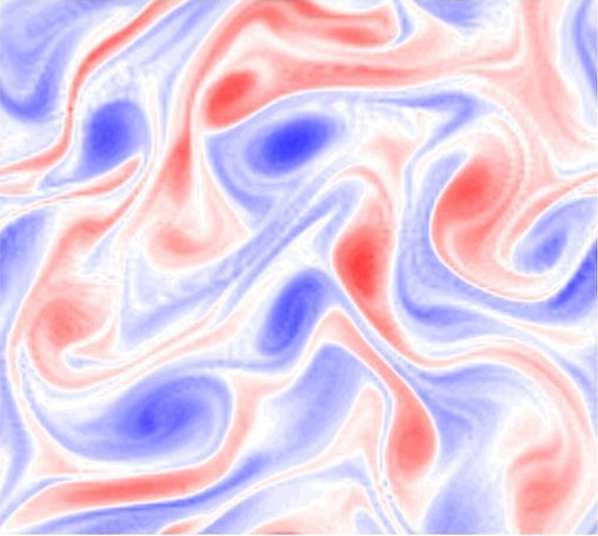
that the SGS terms are preserved under some coordinate transformations, resulting from properties
of the Navier-Stokes equations [2]; see Appendix A for more details. Physical constraints such as
conservation laws can also be included through an augmented loss function - the optimization target
during training [e.g., 64, 65, 75–77]. Finally, physical constraints can also be enforced in the neural
network architecture, e.g., by modifying particular layers [29, 78] or using special components such
as equivariance-preserving spatial transformers [79–81].

     Building on these earlier studies, here we aim to examine the effectiveness of three methods
for incorporating physics into the learning of non-local, data-driven SGS closure models, with a
particular focus on the performance in the small-data regime. The three methods employed here
are:

 (a) DA, for incorporating rotational equivariances into the input and output training samples,

 (b) Physics-constrained loss function that enforces a global enstrophy constraint (EnsCon),

    (c) Group CNN (GCNN), a type of equivariance-preserving CNN that has rotational symmetries
        (equivariances) built into its architecture.

The test case here is a deterministically forced 2D-HIT flow. As discussed in the paper, the use
of DA and GCNN are inspired by an example showing the inability of a CNN to account for rota-
tional equivariances in the small-data regime, while the use of EnsCon is motivated by the success
of similar global energy constraints in improving the performance of reduced-order and closure
models in past studies [50, 65]. We examine the accuracy of the learnt closure models in a priori
(offline) tests, in terms of both predicting the SGS terms and capturing inter-scale transfers, and
the accuracy and stability of LES with these SGS models in a posteriori (online) tests, with regard
to long-term statistics.

    The remaining sections of this paper are as follows. Governing equations of the forced 2D-HIT
system, the filtered equations, and the DNS and LES numerical solvers are presented in Section 2.
The CNNs and their a priori performance trained in the small- and big-data regimes are discussed
in Section 3. The physics-constrained CNN models (DA, GCNN, and EnsCon) are described in
Section 4. Results of the a priori and a posteriori tests with these CNNs in the small data regime
are shown in Section 5. Conclusions and future work are discussed in Section 6.

2      DNS and LES: Equations, numerical solvers, and filterings
2.1     Governing equations
As the testbed, we use forced 2D-HIT, which is a fitting prototype for many large-scale geophysical
and environmental flows (where rotation and/or stratification dominate the dynamics). This system
has been widely used as a testbed for novel techniques, including ML-based SGS modeling [e.g., 82–
86]. The dimensionless governing equations in the vorticity (ω) and streamfunction (ψ) formulation
in a doubly periodic square domain with length L = 2π are:

                               ∂ω              1 2
                                  + N (ω, ψ) =    ∇ ω − f − rω,                                   (1a)
                               ∂t              Re
                                       ∇2 ψ = −ω.                                                 (1b)

                                                  3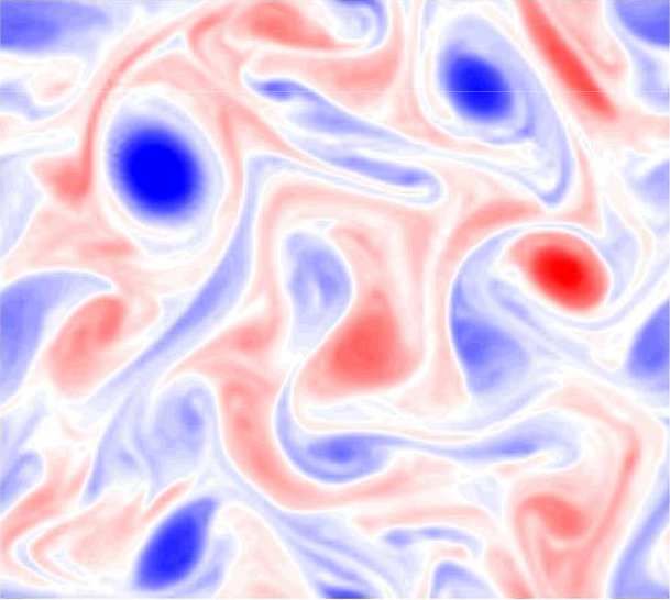
Here, N (ω, ψ) represents the nonlinear advection term:

                                                  ∂ψ ∂ω ∂ψ ∂ω
                                    N (ω, ψ) =          −       ,                                (2)
                                                  ∂y ∂x   ∂x ∂y

and f represents a deterministic forcing [e.g., 83, 86]:

                               f (x, y) = kf [cos (kf x) + cos (kf y)].                          (3)

We study 5 cases, in which the the forcing wavenumber (kf ) and linear friction coefficient (r) have
been varied, creating a variety of flows that differ in dominant length scales and energy/enstrophy
cascade regimes (Figure 1). For all cases, the Reynolds number (Re) is set to 20, 000. In DNS, as
discussed in Section 2.2, Eqs. (1a)-(1b) are numerically solved at high spatio-temporal resolutions.

   To derive the equations for LES, we apply Gaussian filtering [2, 3, 20], denoted by (·), to
Eqs. (1a)-(1b) to obtain

                    ∂ω                   1 2
                       + N (ω, ψ) =         ∇ ω − f − rω + N (ω, ψ) − N (ω, ψ),                (4a)
                    ∂t                   Re                |        {z       }
                                                                          Π
                                2
                              ∇ ψ = −ω.                                                        (4b)

The LES can be solved using a coarser resolution (compared to DNS) with the SGS term Π being
the unclosed term, requiring a closure model.

2.2   Numerical simulations
In DNS, we solve Eqs. (1a)-(1b). A Fourier-Fourier pseudo-spectral solver is used along with
second-order Adams-Bashforth and Crank-Nicolson time-integration schemes for the advection and
viscous terms, respectively [20]. The computational grid has uniform spacing ∆DNS = L/NDNS ,
where NDNS = 1024 is the number of grid points in each direction. The time-stepping size is
set as ∆tDNS = 5 × 10⁻⁵ dimensionaless time unit for all cases except for Case 5, for which
∆tDNS = 2 × 10⁻⁵ is used. For each case, using different random initial conditions, we conducted 3
independent DNS runs to generate the training, offline testing, and online testing datasets. Once
the flow reaches statistical equilibrium after a long-term spin-up, each DNS run produces 2000
snapshots, with each consecutive snapshots 1000∆tDNS apart to reduce the correlation between
training samples (inter-sample correlation cin , or the correlation coefficient between two consecu-
tive Π, is below 0.75; see Section 3 for further discussions). We have also retained data sampled at
25∆tDNS intervals to examine the effect of cin .

    For LES, we solve Eqs. (4a)-(4b) employing the same numerical solver used for DNS, but with
grid resolutions NLES (= NDNS /16 or NDNS /8) listed in Figure 1; for each case ∆tLES = 10∆tDNS .
The SGS term Π is parameterized using a data-driven closure model that is a physics-agnostic or
physics-constrained CNN (Sections 3 and 4) or a physics-based dynamic Smagorinsky model (DS-
MAG). For DSMAG, positive clipping is used to enforce non-negative eddy-viscosity, thus providing
stable a posteriori LES [19, 20].

                                                  4
Case 1: kf = 4 Case 2: kf = 4 Case 3: kf = 10 Case 4: kf = 10 Case 5: kf = 25
r = 0.1, NLES = 64 r = 0.1, NLES = 128 r = 0.1, NLES = 64 r = 0.01, NLES = 64 r = 0.1, NLES = 128
−25 0 25 −25 0 25 −50 0 50 −60 0 60 −80 0 80
DNS
FDNS
CNN
DSMAG
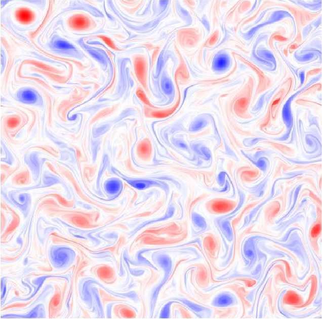
Figure 1: (a) Examples of vorticity fields of DNS, FDNS, and LES with SGS terms modeled by CNN and
DSMAG for 5 cases of forced 2D turbulence with different forcing wavenumber kf , friction coefficient r, and
LES resolution NLES . For all cases, Re = 20, 000 and NDN S = 1024. The scales of the flow structures depend
on kf ; the higher the kf the smaller the scales. The linear drag coefficient r determines the similarity of the
flow structure. When r = 0.1, the flow contains several large vortices of similar sizes, while with r = 0.01
(Case 4), often two large vortices rotating in opposite directions dominate, co-existing with smaller vortices.
For the LES, the CNN is trained on big data (number of training snapshots: ntr = 2000, cin < 0.75) to ensure
accuracy and numerical stability. DSMAG, in general, captures the large-scale structures but underpredicts
the vorticity magnitudes due to the excessive dissipation produced by the non-negative eddy viscosity.
2.3 Filtered DNS (FDNS) data
To obtain the FDNS and to construct the training and testing data for data-driven methods, we
apply a Gaussian filter and then coarse-grain the filtered variables to the LES grid, generating ψ, ω,
and Π [2, 3]. The filtering and coarse-graining process is described in detail in our recent paper [20],
and is only briefly described here. i) Spectral transformation: transform the DNS variables into the
spectral space by Fourier transform; ii) Filtering: apply (element-wise-multiply) a Gaussian filter
kernel (with filter size ∆F = 2∆LES ) in the spectral space to filter the high-wavenumber structures
(the resulting variables still have the DNS resolution); iii) Coarse-graining: truncate the wavenum-
bers greater than the cut-off wavenumber (kc = π/∆LES ) of the filtered variables in the spectral
space ((the resulting variables have the LES resolution); iv) Spectral transformation: transfer the
5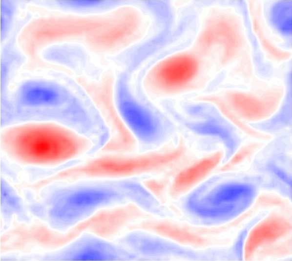
filtered, coarse-grained variables back to the physical space by inverse Fourier transform.

3      Convolutional neural network (CNN): Architecture and results
3.1     Architecture
In this work, we first parameterize the unclosed SGS term Π in (4a) using a physics-agnostic CNN
(CNN hereafter) described in this section. The CNN used in this work has the same architecture
as the one used in our previous study [20], which is 10-layer deep with fully convolutional layers,
i.e., no pooling or upsampling. All layers are randomly initialized and trainable. The convolutional
depth is set to be 64, and the convolutional filter size is 5 × 5. We have performed extensive trial
and error analysis for these hyperparameters to prevent over-fitting while maintaining accuracy.
For example, a CNN with more than 12 layers overfits on this dataset while a CNN with less than
8 layers results in significantly lower a priori correlation coefficients. The activation function of
each layer is the rectified linear unit (ReLU) except for the final layer, which is a linear map.

      We have standardized the input samples as
                               (                      )
                                   ψ/σψ , ω/σω            ∈ R2×NLES×NLES ,                       (5)

and the output samples as
                                       (          )
                                           Π/σΠ       ∈ RNLES×NLES ,                             (6)

where σψ , σω , and σΠ are the standard deviations of ψ, ω, and Π calculated over all training
samples, respectively. In the later sections, we omit σ for clarity, but we always standardize the
input/output samples. The CNN is trained as an optimal map M between the inputs and outputs
                     n             o                             n      o
                  M : ψ/σψ , ω/σω ∈ R2×NLES ×NLES → Π/σΠ ∈ RNLES ×NLES ,                         (7)

by minimizing the mean-squared-error (M SE) loss function
                                        ntr
                                     1 X
                             M SE =         k ΠCNN
                                               i   − ΠFDNS
                                                      i    k22 ,                                 (8)
                                    ntr i=1

where ntr is the number of training samples and k · k2 is the L2 norm.

3.2     Results
 Figure 1 shows examples of vorticity fields from DNS and FDNS, and from a posteriori LES that
uses CNN or DSMAG for the 5 cases. The CNN used here is trained on the full dataset (2000
snapshots with cin < 0.75), which we will refer to as “big data” hereafter. Qualitatively, the LES
with CNN more closely reproduces the small-scale features of FDNS compared to DSMAG. To
better compare the a posteriori performance, Figure 2 shows the turbulent kinetic energy (TKE)
spectra Ê(k) and the probability density functions (PDF) of ω averaged over 100 randomly chosen

                                                            6
snapshots from LES (spanning 2 × 10⁵ ∆tLES or equally 2 × 10⁶ ∆tDNS ) for 3 representative cases (1,
4, and 5). Note that in forced 2D turbulence, according to the classic Kraichnan-Leith-Batchelor
(KLB) similarity theory [87–90], the energy injected by the forcing at wavenumber kf is transferred
to the larger scales (k < kf , energy inverse cascade) while the enstrophy redistributes to the smaller
scales (k > kf , enstrophy forward cascade). The KLB theory predicts a k−5/3 slope of the TKE
spectrum for k < kf and k−3 slope for k > kf .

    In general, the Ê(k) of LES with CNN better matches the FDNS than that of the LES with
DSMAG. For Cases 1 and 4, where the enstrophy forward cascade dominates, the LES with DS-
MAG incorrectly captures the spectra at small scales. For Case 5, where the energy inverse cascade
is important too, the DSMAG fails to recover the energy at large scales correctly. Examining
the PDFs of ω shows that in Cases 4 and 5, the PDF from LES with CNN almost overlaps with
the one from FDNS even at the tails, while the PDF from LES with DSMAG deviates beyond
3 standard deviations. Due to the excessive dissipation, the LES with DSMAG is incapable of
capturing the extremes (tails of the PDF). Therefore, in a posteriori analysis, similar to decaying
2D turbulence [20], for different setups of forced 2D turbulent flows, LES with CNN trained with
big data better reproduces the FDNS flow statistics as compared to LES with DSMAG. Note that
in this study, we are comparing the CNN-based closures against DSMAG, which is more accurate
and powerful than the typical baseline, the static Smagorinsky model [20, 39]. Finally, we highlight
that the CNN has outstanding a priori performance too, yielding c > 0.9 (Figure 3).

     Although the CNNs yield outstanding performance in both a priori and a posteriori analyses
when trained with big data, their performance deteriorates when the training dataset is small.
Before introducing three physics-constrained CNNs for overcoming this problem (Section 4), we
first show in Figure 3 classifying that “big” versus “small” data depends not only on the number
of snapshots in the training dataset (ntr ) but also on the inter-sample correlation (cin ). In a priori
analysis (bar plots in Figure 3), we use four metrics. The first two are cin , which is the average
correlation coefficient between consecutive snapshots of Π in the training set, and c, which is the
average correlation coefficient between the true (FDNS) and CNN-predicted Π over 100 random
snapshots in the testing set. Following past studies [20, 39], we introduce

                                       T = sgn(∇2 ω) ⊙ Π,                                           (9)

whose sign at a grid point determines whether the SGS term is diffusive T > 0 or anti-diffusive T < 0
(⊙ denotes element-wise multiplication). The third metric we use is c computed separately based
on the sign of T for testing samples: cT >0 , which is the average c on the grid points experiencing
diffusion by SGS processes and cT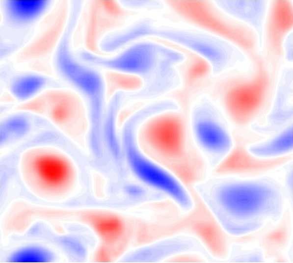
this datasets is 40 times longer than the other two).

    The a priori results show that CNN50                    2000
                                         small data and CNNsmall data have comparable c, cT >0 , cT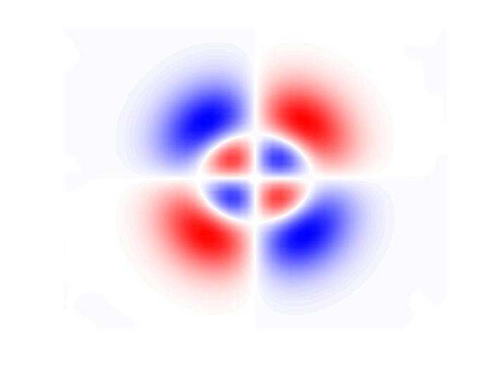
Ê(k)                                                  PDF
                                                        1091
                         k−3
 100                                    Case 1                                                 Case 1
                                                        1092

                                                        1093
1095         DNS
             FDNS                                       1094

             CNN
                                                        1095
10910        DSMAG

                                                        1096
                10                102                       -10          -5         0          5         10
                                                        1091
                         k−3
 100                                    Case 4                                                 Case 4
                                                        1092

                                                        1093

1095                                                    1094

                                                        1095

10910                                                   1096

                                                        1097
                10                102                      -15     -10        -5    0      5       10   15
                                                        1091
                 k−5/3
 100                            k−3     Case 5          1092                                   Case 5

                                                        1093

                                                        1094
1095
                                                        1095

                                                        1096

10910                                                   1097

                                                        1098
                10               102                        -10          -5          0         5         10
                     k=   (kx2 + ky2 )0.5                                          ω/σω
Figure 2: Turbulent kinetic energy (TKE, Ê(k)) spectra and probability density functions (PDFs) of ω for repre-
sentative cases (1, 4, and 5). The CNNs used here are trained on big data. The spectra and PDFs are averaged over
100 samples from the testing set. The PDF is calculated using a kernel estimator [91].

                                                       9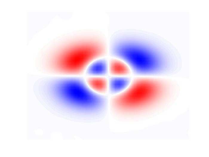
(a) Case 1: A priori analysis                                    (b) Case 1: Ê(k)
 1.0                                                        CNN50            100
                                                               small data
 0.8
                                                            CNN2000
                                                               small data
 0.6                                                                        1094
                                                                                   FDNS
                                                            CNN2000
                                                               big data            CNN50
 0.4                                                                                  small data

                                                                                   CNN2000
                                                                                      small data
 0.2                                                                               CNN2000
                                                                                      big data
                                                                            1098
    0
                                                                                          101           102

                    (c) Case 3: A priori analysis                                    (d) Case 3: Ê(k)
 1.0
                                                                             100
 0.8

 0.6
                                                                            1093
 0.4

 0.2

    0                                                                       1097
          cin            c          cT >0         cT
ω̄ ΠFDNS ΠCNN ΠDA ΠGCNN
(a)
90 90 ⇓ 90 90
(b)
Figure 4: A dipole vortex shows the shortcoming of a physics-agnostic CNN in capturing the rotational
equivariance of the SGS term (third column). The physics-agnostic CNN regards the rotational transform
between the training and testing vortex field as a translational transform (the translation of the structure
in the black dashed box). However, the CNN with DA or GCNN can capture this rotational equivariance
correctly (fourth and fifth columns). The symbol 90 means rotation by 90◦ clockwise and ⇓ means translation.
of the two parts of the vertically aligned dipole (third column, second row)2 .
The implication of this example is that if the training set only involves limited flow config-
urations (i.e., small-data regime) such as only those from the first row, then the CNN can be
quite inaccurate for a testing set involving new configurations such as those in the second row. In
the much more complicated 2D-HIT flow, there are various complex flow configurations. In a big
training set, it is more likely that these different configurations would be present and the CNN
learns their corresponding Π terms and the associated transformations; however, this is less likely
in a small training set. The SGS term Π is known to be equivariant to translation and rotation,
i.e., if the flow state variables are translated or rotated, Π should also be translated or rotated
to the same degree [2]. While translation equivariance is already achieved in a regular CNN by
weight sharing [92], rotational equivariance is not guaranteed. Recent studies show that rotational
equivariance can actually be critical in data-driven SGS modeling [27, 66, 69, 74]. To capture the
rotational equivariance in the small-data regime, we propose two separate approaches: (1) DA,
by including 3 additional rotated (by 90◦ , 180◦ , and 270◦ ) counterparts of each original FDNS
snapshot in the training set [74] and (2) by using a GCNN architecture, which enforces rotational
equivariance by construction [92, 93].
The GCNN uses group convolutions, which increases the degree of weight sharing by transform-
ing and reorienting the filters such that the feature maps in GCNN are equivariant under imposed
symmetry transformations, e.g., rotation and reflection [94]. In our work, the group convolutional
filters are oriented at 0◦ , 90◦ , 180◦ , and 270◦ such that the feature map and the output (ΠGCNN )
are rotationally equivariant with respect to the inputs (ψ̄ and ω̄), i.e., Eq. (15) in Appendix A.
In addition to the structural modeling approaches mentioned above that achieve rotational
2
The CNN basically predicts that because the red blob of the dipole is now to the left of the blue blob, the part
of the Π term corresponding to the red blob in the first row now should be to the right of the part corresponding to
the blue blob (see the black box in the third column).
11equivariance (still with the MSE loss function, Eq. (8)), we can also modify the loss function to
combine structural and functional modeling approaches to enhance the performance of CNN in
the small-data regime. For example, in 2D turbulence, the SGS enstrophy transfer is critical in
maintaining the accuracy and stability of LES [20, 39, 95]. Therefore, capturing the correct SGS
enstrophy transfer hωΠi in a CNN can be important for its performance. The a priori analysis in
Figure 3 already showed that the error in capturing the global SGS enstrophy transfer ǫ is small in
the big-data regime, but can be large in the small-data regime. Here we propose to add a penalty
term to the loss function that acts as regularization, enforcing (as a soft constraint) the global SGS
enstrophy transfer. Similar to the global energy constraint implemented in Ref. [65], this physics-
constrained loss function consist of the MSE plus the global SGS enstrophy transfer error:
ntr ntr
1−β X β X
Loss = k ΠCNN
i − ΠFDNS 2
i k2 + |hω i ΠCNN
i i − hω i ΠFDNS
i i|, (11)
ntr i=1 ntr i=1
where β ∈ [0, 1] is an adjustable hyperparameter. We empirically find β = 0.5 to be optimal in
minimizing the relative total enstrophy transfer error (ǫ) without significantly affecting c. This
physics-constrained loss function (Eq. (11)) synergically combines the structural and functional
modeling approaches.
5 Results
5.1 A priori analysis
A priori analysis is performed using the following metrics: correlation coefficients (c), global enstro-
phy transfer error (ǫ), and scale-dependent enstrophy and energy transfers (TZ and TE , as defined
later in this section). Figure 5 shows the bar plots of c, cT 0 , and ǫ for 3 representative
cases (1, 3, and 4). In the small-data regime (ntr = 50), the use of DA or GCNN increases the
correlation coefficients c, cT 0 ; the increases are largest for cT >0 , whose low values could
lead to instabilities in a posteriori LES, as discussed earlier. The use of DA or GCNN also decreases
the relative total enstrophy transfer error ǫ, particularly for Case 1. One point to highlight here
is that DA can achieve the same, and in some cases even better, a priori accuracy compared to
GCNN, while the network architecture is much simpler in DA, which builds equivariance simply in
the training data. The EnsCon does not improve the correlation coefficient c (because it only adds
a functional modeling component), but as expected, it decreases ǫ, which as shown later improves
the a posteriori LES. To examine a combined approach, we build an enstrophy-constrained GCNN
(GCNN-EnsCon), which performs somewhere in between GCNN and EnsCon: GCNN-EnsCon has
a higher c than EnsCon but lower than GCNN, and GCNN-EnsCon has higher ǫ than EnsCon
but lower than GCNN. As shown later, the LES with GCNN-EnsCon has the best a posteriori
performance among all tested models.
To summarize Figure 5, the physics-constrained CNNs trained on small data (ntr = 50) out-
perform the physics-agnostic CNN trained on small data, but none could outperform the physics-
agnostic CNN trained on 40 times more data (ntr = 2000) in these a priori tests. However, we
emphasize that 40 is a substantial factor in terms of the amount of high-fidelity data. This figure
also shows that adding physics constraints to the CNN trained in the big-data regime (ntr = 2000)
does not necessarily lead to any improvement over CNN2000 , suggesting that these physics con-
12straints could be learnt by a physics-agnostic CNN from the data given enough training samples.
To further assess the performance of the closures computed using physics-constrained CNNs
trained in the small-data regime, we also examine the scale-dependent enstrophy and energy trans-
fers (TZ and TE ) defined as: [84, 96]
ˆ k ),
TZ (k) = R(−Π̂∗k ω̄ (12)
T (k) = R(−Π̂∗ ψ̄ˆ ).
E k k (13)
ˆ denotes Fourier transform, and the asterisks denote com-
Here, R(·) means the “real part of”, (·)
plex conjugate. The scale-dependent enstrophy/energy transfer is positive for enstrophy/energy
backscatter (enstrophy/energy moving from subgrid scales to resolved scales) and negative for en-
strophy/energy forward transfer (enstrophy/energy moving from resolved scales to subgrid scales) [96].
Note that backscatter and forward transfer here are inter-scale transfers by the SGS term (Π), and
are different concepts from inverse and forward cascades (discussed earlier in Section 3.2).
Figure 6 shows the power spectra of |Π̂(k)|2 , TZ , and TE from FDNS and different CNNs,
providing further evidence that the incorporated physics constraints improves the a priori perfor-
mance of the data-driven closures. For Case 1 (first row), the |Π̂(k)|2 is better predicted by DA
and GCNN at the high wavenumbers. The scale-dependent enstrophy forward transfer (TZ < 0 in
Figure 6(b)) is underpredicted by CNN, and the deviation from FDNS is corrected by DA, GCNN,
EnsCon, and GCNN-EnsCon. For Case 5 (second row), however, where the inverse energy cascade
is important (see Section 3.2), the gain from the physicss-constrained CNNs (DA, GCNN, EnsCon,
and GCNN-EnsCon) can be seen in the scale-dependent energy transfer (TE in Figure 6(f)), where
the physics-agnostic CNN incorrectly predicts a portion (k < 4) of energy backscatter (TE > 0) to
be forward energy transfer (TE < 0).
5.2 A posteriori analysis
Figures 7-9 show the Ê(k) spectra of Cases 1-5 . In general, the TKE spectrum from LES with
the physics-agnostic CNN (denoted by CNN50 ) matches the one from FDNS at low wavenumbers
(large-scale structures) but severely over-predicts the TKE at high wavenumbers (small-scale struc-
tures). For example, CNN50 starts to deviate from FDNS at k ≈ 20 for Cases 1, 3, and 4 as shown
in Figure 7 (left) and Figure 8. This over-prediction can lead to unphysical and unstable numerical
results. For example, the vorticity field of LES with CNN50 exhibits extensive noisy (i.e., very high-
wavenumber) structures in several simulations (not shown). All LES runs with physics-constrained
CNNs (DA50 , GCNN50 , EnsCon50 , and GCNN-EnsCon50 ) outperform the LES with CNN50 . In
particular, for Cases 2 (Figure 7 (right)) and 3 (Figure 8 (left)), the LES runs with DA50 , GCNN50 ,
EnsCon50 , and GCNN-EnsCon50 produce similar TKE spectra which are consistently better than
that of the LES with CNN50 . For Cases 1 (Figure 7 (left)) and 4 (Figure 8 (right)), however,
incorporating rotational equivariance (through DA, GCNN, or GCNN-EnsCon) leads to better a
posteriori performances than incorporating the global enstrophy constraint alone (EnsCon) in terms
of matching the FDNS spectra. Overall, the LES with GCNN-EnsCon50 has the best performance
in these 4 cases, showing the advantage of combining different types of physics constraints in the
small-data regime.
In Case 5, the gain from the physics constraints is less obvious from the TKE spectra, although
a slight improvement at the tails can still be observed (Figure 9 (left)). In this case, the PDF
13CNN50 EnsCon50 DA50 GCNN50 GCNN-EnsCon50 CNN2000 DA2000 GCNN2000
1.0
Case 1
0.5
0
1.0
Case 3
0.5
0
1.0
Case 4
0.5
0 c cT >0 cT 0 , and cT >0 , and the relative enstrophy
transfer error ǫ. It is shown that EnsCon does not improve the structural modeling metric c but significantly
reduces the functional modeling error, ǫ. DA and GCNN enhance the structural modeling performance and
also reduce ǫ. The superscripted number denotes the ntr in the training dataset with cin < 0.75 as in
Figure 3. The error bars denote plus and minus one standard deviation (the error bars on ǫ are small and
not shown for the sake of clarify).
of vorticity (Figure 9 (right)) better reveals the gain, where LES with CNN50 predicts spuriously
large vorticity extremes due to the excessive high-wavenumber structures in the vorticity field. The
physics-constrained CNNs (DA50 , GCNN50 , EnsCon50 , and GCNN-EnsCon50 ) result in a stable
and more accurate LES as the TKE spectrum and PDF of vorticity better match those of the
FDNS.
6 Summary and discussion
The objective of this paper is to learn CNN-based non-local SGS closures from filtered DNS data
for stable and accurate LES, with a focus on the small-data regime, i.e., when the available DNS
training set is small. We demonstrate that incorporating physics constraints into the CNN using
three methods can substantially improve the a priori (offline) and a posteriori (online) performance
of the data-driven closure model in the small-data regime.
We use 5 different forced 2D homogeneous isotropic turbulence (HIT) flows with various forcing
wavenumbers, linear drag coefficients, and LES grid sizes as the testbeds. First, we show in Sec-
tion 3 that in the “big-data” regime (with ntr = 2000 weakly correlated training samples), the LES
with physics-agnostic CNN is stable and accurate, and outperforms the LES with the physics-based
DSMAG closure, particularly as the data-driven closure captures backscattering well (see Figure 2
and Ref. [20]). Next, we show, using a priori (offline) and a posteriori (online) tests, that the
14|Π̂(k)|2 TZ (k) TE (k)
Case 1 (a) (b) (c)
k 2.46 1092
0.1
100
FDNS
0 0
CNN50
1092
EnsCon50
DA50
90.1
GCNN50
91092
10 94
GCNN-EnsCon50
10 50 10 50 10 50
Case 5 (d) (e) (f)
k 2.46 2 0.4
100
1 0.2
0 0
1092
91 90.2
92 90.4
1094
10 100 10 100 10 100
k k k
Figure 6: A priori analysis in terms of scale-dependent power spectra |Π̂(k)|2 , and scale-dependent enstrophy
and energy transfers TZ and TE for two representative cases (1 and 5). The inertial part of the |Π̂(k)|2
spectrum has a slope of 2.46, consistent with previous studies [96, 97]. (a)-(c): In Case 1 where the enstrophy
direct cascade is important (as discussed in Section 3.2), CNN50 does not capture the power spectra correctly
at high wavenumbers, and the enstrophy forward transfer (TZ < 0) is under-predicted. (d)-(f): In Case 5
where the energy inverse cascade is important (see Section 3.2), the prediction discrepancy occurs at the
low wavenumbers of the power spectra, and at the backscattering part of the energy transfer (TE > 0).
In general, the proposed physics-constrained CNNs (DA, GCNN, EnsCon, and GCNN-EnsCon) reduce the
prediction error in both structural (|Π̂(k)|2 ) and functional (TZ and TE ) modelings metrics.
performance of the physics-agnostic CNNs substantially deteriorate when they are trained in the
“small-data” regime: with ntr = 2000 highly correlated samples or with ntr = 50 weakly correlated
samples. This analysis demonstrates that the small versus big data regime depends not only on
the number of training samples but also on their inter correlations.
To improve the performance of CNNs trained in the small-data regime, in Section 4, we propose
incorporating physics in the CNNs through using 1) data augmentation (DA), 2) a group equivariant
CNN (GCNN), or an enstrophy-constrained loss function (EnsCon). The idea behind using DA
and GCNN is to account for the rotational equivariance of the SGS term. This is inspired by a
simple example of a vortex dipole, which shows that for never-seen-before samples, the physics-
agnostic CNN can only capture the translational equivariance, but not the rotational equivariance,
another important property of the SGS term. The idea behind EnsCon is to combine structural and
functional modeling approaches through a regularized loss function. A priori and a posteriori tests
show that all these physics-constrained CNNs outperform the physics-agnostic CNN in the small-
data regime (ntr = 50). Improvements of the data-driven SGS closures using the GCNN, which
uses an equivariant-preserving architecture, are consistent with the findings of a recent study [69],
though it should be mentioned that DA, which simply builds equivariance in the training samples
and can be used with any architecture, shows comparable or even in some cases better performance
than GCNN.
15Ê(k) Ê(k)
100 Case 1 100 Case 2
FDNS
CNN50
1095 EnsCon50 1095
DA50
GCNN50
GCNN-EnsCon50
10910 10910
100 101 102 100 101 102
k k
Figure 7: The TKE spectra Ê(k) of Cases 1 and 2 from a posteriori LES run. Results are from long-term
LES integrations (2×10⁵ ∆tLES or 2×10⁶∆tDNS ). The Ê(k) is calculated from 100 randomly chosen snapshots
and then averaged. The insert in Case 2 magnifies the tails of the Ê(k) spectra for better visualization. In
general, the physics-constrained CNNs (DA50 , GCNN50 , EnsCon50 , or GCNN-EnsCon50 ) improve the a
posteriori performance of LES compared to the LES with the physics-agnostic CNN50 : The spectra from the
LES with physics-constrained CNNs better match the FDNS spectra especially at the tails (high-wavenumber
structures). In particular, the spectra from the LES with GCNN-EnsCon50 have the best match with the
FDNS spectra especially at the high wavenumbers. The improvement is more prominent for the coarser-grid
LES (Case 1, NLES = 64, compared to Case 2, NLES = 128).
Overall, GCNN+EnsCon, which combines these two main constraints, demonstrate the best a
posteriori performance, showing the advantage of adding physics constraints together. Note that
here we focus on rotational equivariance, which is a property of the 2D turbulence test case. In
other flows, other equivariance properties might exist (e.g., reflection equivariance as in Couette flow
and Rayleigh Bénard convection), and they can be incorporated through DA or GCNN as needed.
These results show the major advantage and potential of physics-constrained deep learning methods
for SGS modeling in the small-data regime, which is of substantial importance for complex and
high-Reynolds number flows, for which the availability of high-fidelity (e.g., DNS) data could be
severely limited.
Acknowledgments
This work was supported by an award from the ONR Young Investigator Program (N00014-20-
1-2722), a grant from the NSF CSSI program (OAC-2005123), and by the generosity of Eric and
Wendy Schmidt by recommendation of the Schmidt Futures program. Computational resources
were provided by NSF XSEDE (allocation ATM170020) and NCAR′ s CISL (allocation URIC0004).
Our codes and data are available at https://github.com/envfluids/2D-DDP.
16Ê(k) Ê(k)
100 Case 3 100 Case 4
FDNS
CNN50
1095 EnsCon50 1095
DA50
GCNN50
GCNN-EnsCon50
10910 10910
100 101 102 100 101 102
k k
Figure 8: Same as Figure 7 but for Cases 3 and 4. Similar to the finding of Figure 7, the physics-
constrained CNNs (DA50 , GCNN50 , EnsCon50 , or GCNN-EnsCon50 ) improve the a posteriori performance
of LES compared to the LES with the physics-agnostic CNN50 . For Case 3, the improvement can only
be observed at the highest wavenumber. For Case 4, however, incorporating the rotational equivariance
(DA50 , GCNN50 , and GCNN-EnsCon50 ) leads to a more accurate LES than the enstrophy constraint alone
(EnsCon50 ) alone. Also similar to the finding of Figure 7, the spectra from the LES with GCNN-EnsCon50
have the best match with the FDNS spectra especially at the high wavenumbers.
(a) Ê(k) (b) PDF
100
100 Case 5 Case 5
1092
FDNS
1094
1095 CNN50
EnsCon50
1096 DA50
GCNN50
GCNN-EnsCon50
10910
10 98
100 101 102 910 95 0 5 10
k ω̄/σω̄
Figure 9: Same as Figure 7 but showing (a) The TKE spectra Ê(k) and (b) probability density function
(PDF) of ω for Case 5. Although, the physics-constrained CNNs (DA50 , GCNN50 , EnsCon50 , or GCNN-
EnsCon50 ) result in slightly improved LES in terms of the TKE spectrum, the gain from the physical
constraints can be observed more clearly in the PDF of vorticity where the LES with CNN50 over-predicts
the extreme values (tails of the PDF).
17A Appendix: Equivariance properties of the SGS term
According to the transformation properties of the Navier-Stokes equations [2], the SGS term Π
should satisfy:
Π(Tg ω, Tg ψ) = Tg Π(ω, ψ), (14)
where Tg represents a translational or rotational transformation. ω and ψ are the vorticity and
streamfunction, respectively (as described in Section 2).
In the ML literature, “equivariance” means that transforming an input (e.g., by translation or
rotation, denoted by Tg ) and then passing the transformed input through the learnt map (CNN
in our case) should give the same result as first mapping the input and then transforming the
output [92, 94]:
ΠCNN (Tg ω̄, Tg ψ̄, θ) = Tg ΠCNN (ω̄, ψ̄, θ). (15)
Here, θ represents a group of learnable parameters of the network. To preserve the translational and
rotational equivariance of Π (Eq. (14)), the network parameters θ should be learnt such that Eq. (15)
is satisfied. In turbulence modeling, “equivariance” may also be referred to as “symmetry” [2, 73].
In this paper, we use the term “equivariance”, and use an equivarience-preserving network (GCNN)
or build this property into the training via DA.
B Appendix: The global enstrophy-transfer constraint
The equation for enstrophy transfer can be obtained by first multiplying the filtered equation (Eq. (4a))
by ω:
∂ω 1
ω + ωN (ω, ψ) = ω ∇2 ω − ωf − rω2 + ωN (ω, ψ) − ωN (ω, ψ) . (16)
∂t Re | {z }
ωΠ
Rearranging Eq. (16) gives:
1 ∂ω 2 1 1 1 2 2
+ N (ω 2 , ψ) = ∇ ω − (∇ω)2 − ωf − rω 2 + ωΠ. (17)
2 ∂t 2 Re 2
The evolution equation for domain-averaged enstrophy Z = h 21 ω 2 i is then obtained by domain
averaging Eq. (17) and invoking the domain’s periodicity [98]:
dZ 1
= − h(∇ω)2 i − hωf i − 2rZ + hωΠi. (18)
dt Re
Therefore, the domain-averaged enstrophy transfer due to the SGS term is hωΠi. In Eq. (11), we
enforce hωΠi predicted by the CNN to be close to that of the FDNS as a domain-averaged (global)
soft constraint.
18References
[1] J. Smagorinsky, General circulation experiments with the primitive equations: I. The basic experiment,
Monthly Weather Review 91 (3) (1963) 99–164.
[2] S. B. Pope, Turbulent Flows, IOP Publishing, 2001.
[3] P. Sagaut, Large eddy simulation for incompressible flows: An introduction, Springer Science & Business
Media, 2006.
[4] R. D. Moser, S. W. Haering, G. R. Yalla, Statistical properties of subgrid-scale turbulence models,
Annual Review of Fluid Mechanics 53.
[5] E. Bou-Zeid, C. Meneveau, M. Parlange, A scale-dependent Lagrangian dynamic model for large eddy
simulation of complex turbulent flows, Physics of Fluids 17 (2) (2005) 025105.
[6] P. Sagaut, M. Terracol, S. Deck, Multiscale and multiresolution approaches in turbulence-LES, DES
and Hybrid RANS/LES methods: Applications and Guidelines, World Scientific, 2013.
[7] T. Schneider, S. Lan, A. Stuart, J. Teixeira, Earth system modeling 2.0: A blueprint for models that
learn from observations and targeted high-resolution simulations, Geophysical Research Letters 44 (24)
(2017) 12–396.
[8] L. Zanna, T. Bolton, Deep Learning of Unresolved Turbulent Ocean Processes in Climate Models, Deep
Learning for the Earth Sciences: A Comprehensive Approach to Remote Sensing, Climate Science, and
Geosciences (2021) 298–306.
[9] A. Leonard, Energy cascade in large-eddy simulations of turbulent fluid flows, in: Advances in geo-
physics, vol. 18, Elsevier, 237–248, 1975.
[10] R. A. Clark, J. H. Ferziger, W. C. Reynolds, Evaluation of subgrid-scale models using an accurately
simulated turbulent flow, Journal of fluid mechanics 91 (1) (1979) 1–16.
[11] C. Meneveau, J. Katz, Scale-invariance and turbulence models for large-eddy simulation, Annual Review
of Fluid Mechanics 32 (1) (2000) 1–32.
[12] H. Lu, F. Porté-Agel, A modulated gradient model for scalar transport in large-eddy simulation of the
atmospheric boundary layer, Physics of Fluids 25 (1) (2013) 015110.
[13] A. Vollant, G. Balarac, C. Corre, A dynamic regularized gradient model of the subgrid-scale stress
tensor for large-eddy simulation, Physics of Fluids 28 (2) (2016) 025114.
[14] Y. Wang, Z. Yuan, C. Xie, J. Wang, A dynamic spatial gradient model for the subgrid closure in
large-eddy simulation of turbulence, Physics of Fluids 33 (7) (2021) 075119.
[15] Z. Yuan, Y. Wang, C. Xie, J. Wang, Dynamic iterative approximate deconvolution models for large-eddy
simulation of turbulence, Physics of Fluids 33 (8) (2021) 085125.
[16] M. Germano, U. Piomelli, P. Moin, W. H. Cabot, A dynamic subgrid-scale eddy viscosity model, Physics
of Fluids A: Fluid Dynamics 3 (7) (1991) 1760–1765.
[17] D. K. Lilly, A proposed modification of the Germano subgrid-scale closure method, Physics of Fluids
A: Fluid Dynamics 4 (3) (1992) 633–635.
[18] Y. Zang, R. L. Street, J. R. Koseff, A dynamic mixed subgrid-scale model and its application to turbulent
recirculating flows, Physics of Fluids A: Fluid Dynamics 5 (12) (1993) 3186–3196.
[19] S. Pawar, O. San, A. Rasheed, P. Vedula, A priori analysis on deep learning of subgrid-scale parame-
terizations for Kraichnan turbulence, Theoretical and Computational Fluid Dynamics (2020) 1–27.
[20] Y. Guan, A. Chattopadhyay, A. Subel, P. Hassanzadeh, Stable a posteriori LES of 2D turbulence using
convolutional neural networks: Backscattering analysis and generalization to higher Re via transfer
learning, arXiv preprint arXiv:2102.11400 .
[21] Z. Wang, K. Luo, D. Li, J. Tan, J. Fan, Investigations of data-driven closure for subgrid-scale stress in
large-eddy simulation, Physics of Fluids 30 (12) (2018) 125101.
[22] Z. Zhou, G. He, S. Wang, G. Jin, Subgrid-scale model for large-eddy simulation of isotropic turbulent
flows using an artificial neural network, Computers & Fluids 195 (2019) 104319.
[23] J.-X. Wang, J.-L. Wu, H. Xiao, Physics-informed machine learning approach for reconstructing Reynolds
stress modeling discrepancies based on DNS data, Physical Review Fluids 2 (3) (2017) 034603.
[24] K. Duraisamy, G. Iaccarino, H. Xiao, Turbulence modeling in the age of data, Annual Review of Fluid
Mechanics 51 (2019) 357–377.
[25] R. Maulik, O. San, J. D. Jacob, C. Crick, Sub-grid scale model classification and blending through deep
learning, Journal of Fluid Mechanics 870 (2019) 784–812.
19[26] A. Beck, D. Flad, C.-D. Munz, Deep neural networks for data-driven LES closure models, Journal of
Computational Physics 398 (2019) 108910.
[27] A. Prat, T. Sautory, S. Navarro-Martinez, A Priori Sub-grid Modelling Using Artificial Neural Networks,
International Journal of Computational Fluid Dynamics (2020) 1–21.
[28] S. Taghizadeh, F. D. Witherden, S. S. Girimaji, Turbulence closure modeling with data-driven tech-
niques: physical compatibility and consistency considerations, New Journal of Physics 22 (9) (2020)
093023.
[29] L. Zanna, T. Bolton, Data-Driven Equation Discovery of Ocean Mesoscale Closures, Geophysical Re-
search Letters 47 (17) (2020) e2020GL088376.
[30] S. L. Brunton, B. R. Noack, P. Koumoutsakos, Machine learning for fluid mechanics, Annual Review of
Fluid Mechanics 52 (2020) 477–508.
[31] A. Beck, M. Kurz, A perspective on machine learning methods in turbulence modeling, GAMM-
Mitteilungen 44 (1) (2021) e202100002.
[32] K. Duraisamy, Perspectives on machine learning-augmented Reynolds-averaged and large eddy simula-
tion models of turbulence, Physical Review Fluids 6 (5) (2021) 050504.
[33] N. Moriya, K. Fukami, Y. Nabae, M. Morimoto, T. Nakamura, K. Fukagata, Inserting machine-
learned virtual wall velocity for large-eddy simulation of turbulent channel flows, arXiv preprint
arXiv:2106.09271 .
[34] G. D. Portwood, B. T. Nadiga, J. A. Saenz, D. Livescu, Interpreting neural network models of residual
scalar flux, Journal of Fluid Mechanics 907.
[35] R. Stoffer, C. M. Van Leeuwen, D. Podareanu, V. Codreanu, M. A. Veerman, M. Janssens, O. K.
Hartogensis, C. C. Van Heerwaarden, Development of a large-eddy simulation subgrid model based on
artificial neural networks: a case study of turbulent channel flow, Geoscientific Model Development
14 (6) (2021) 3769–3788.
[36] B. Liu, H. Yu, H. Huang, X.-Y. Lu, Investigation of nonlocal data-driven methods for subgrid-scale
stress modelling in large eddy simulation, arXiv preprint arXiv:2109.01292 .
[37] C. Jiang, R. Vinuesa, R. Chen, J. Mi, S. Laima, H. Li, An interpretable framework of data-driven
turbulence modeling using deep neural networks, Physics of Fluids 33 (5) (2021) 055133.
[38] Y. Tian, D. Livescu, M. Chertkov, Physics-informed machine learning of the Lagrangian dynamics of
velocity gradient tensor, Physical Review Fluids 6 (9) (2021) 094607.
[39] R. Maulik, O. San, A. Rasheed, P. Vedula, Subgrid modelling for two-dimensional turbulence using
neural networks, Journal of Fluid Mechanics 858 (2019) 122–144.
[40] C. Xie, K. Li, C. Ma, J. Wang, Modeling subgrid-scale force and divergence of heat flux of compressible
isotropic turbulence by artificial neural network, Physical Review Fluids 4 (10) (2019) 104605.
[41] C. Xie, J. Wang, K. Li, C. Ma, Artificial neural network approach to large-eddy simulation of compress-
ible isotropic turbulence, Physical Review E 99 (5) (2019) 053113.
[42] C. Xie, J. Wang, H. Li, M. Wan, S. Chen, Artificial neural network mixed model for large eddy simulation
of compressible isotropic turbulence, Physics of Fluids 31 (8) (2019) 085112.
[43] C. Xie, X. Xiong, J. Wang, Artificial neural network approach for turbulence models: A local framework,
arXiv preprint arXiv:2101.10528 .
[44] Y. Wang, Z. Yuan, C. Xie, J. Wang, Artificial neural network-based spatial gradient models for large-
eddy simulation of turbulence, AIP Advances 11 (5) (2021) 055216.
[45] R. Maulik, H. Sharma, S. Patel, B. Lusch, E. Jennings, A turbulent eddy-viscosity surrogate modeling
framework for Reynolds-Averaged Navier-Stokes simulations, Computers & Fluids 227 (2021) 104777.
[46] M. Sonnewald, R. Lguensat, D. C. Jones, P. D. Dueben, J. Brajard, V. Balaji, Bridging observation,
theory
. and numerical simulation of the ocean using Machine Learning, arXiv preprint arXiv:2104.12506
[47] T. Bolton, L. Zanna, Applications of deep learning to ocean data inference and subgrid parameterization,
Journal of Advances in Modeling Earth Systems 11 (1) (2019) 376–399.
[48] M. Kurz, A. Beck, A machine learning framework for LES closure terms, Electronic transactions on
numerical analysis 56 (2022) 117–137.
[49] A. Subel, A. Chattopadhyay, Y. Guan, P. Hassanzadeh, Data-driven subgrid-scale modeling of forced
Burgers turbulence using deep learning with generalization to higher Reynolds numbers via transfer
learning, Physics of Fluids 33 (3) (2021) 031702.
20[50] U. Achatz, G. Schmitz, On the closure problem in the reduction of complex atmospheric models by PIPs
and EOFs: A comparison for the case of a two-layer model with zonally symmetric forcing, Journal of
the atmospheric sciences 54 (20) (1997) 2452–2474.
[51] J.-C. Loiseau, S. L. Brunton, Constrained sparse Galerkin regression, Journal of Fluid Mechanics 838
(2018) 42–67.
[52] Z. Y. Wan, P. Vlachas, P. Koumoutsakos, T. Sapsis, Data-assisted reduced-order modeling of extreme
events in complex dynamical systems, PLOS One 13 (5) (2018) e0197704.
[53] Y. Guan, S. L. Brunton, I. Novosselov, Sparse nonlinear models of chaotic electroconvection, R. Soc.
open sci. 8 (2021) 202367.
[54] A. A. Kaptanoglu, K. D. Morgan, C. J. Hansen, S. L. Brunton, Physics-constrained, low-dimensional
models for magnetohydrodynamics: First-principles and data-driven approaches, Physical Review E
104 (1) (2021) 015206.
[55] R. Vinuesa, S. L. Brunton, The Potential of Machine Learning to Enhance Computational Fluid Dy-
namics, arXiv preprint arXiv:2110.02085 .
[56] M. Khodkar, P. Hassanzadeh, A data-driven, physics-informed framework for forecasting the spatiotem-
poral evolution of chaotic dynamics with nonlinearities modeled as exogenous forcings, Journal of Com-
putational Physics 440 (2021) 110412.
[57] R. Maulik, V. Rao, J. Wang, G. Mengaldo, E. Constantinescu, B. Lusch, P. Balaprakash, I. Foster,
R. Kotamarthi, AIEADA 1.0: Efficient high-dimensional variational data assimilation with machine-
learned reduced-order models, Geoscientific Model Development Discussions (2022) 1–20.
[58] J.-L. Wu, H. Xiao, E. Paterson, Physics-informed machine learning approach for augmenting turbulence
models: A comprehensive framework, Physical Review Fluids 3 (7) (2018) 074602.
[59] R. King, O. Hennigh, A. Mohan, M. Chertkov, From deep to physics-informed learning of turbulence:
Diagnostics, arXiv preprint arXiv:1810.07785 .
[60] R. Sharma, A. B. Farimani, J. Gomes, P. Eastman, V. Pande, Weakly-supervised deep learning of heat
transport via physics informed loss, arXiv preprint arXiv:1807.11374 .
[61] S. Pan, K. Duraisamy, Long-time predictive modeling of nonlinear dynamical systems using neural
networks, Complexity 2018.
[62] A. Chattopadhyay, E. Nabizadeh, P. Hassanzadeh, Analog forecasting of extreme-causing weather pat-
terns using deep learning, Journal of Advances in Modeling Earth Systems 12 (2) (2020) e2019MS001958.
[63] K. Meidani, A. B. Farimani, Data-driven identification of 2D Partial Differential Equations using ex-
tracted physical features, Computer Methods in Applied Mechanics and Engineering 381 (2021) 113831.
[64] T. Beucler, M. Pritchard, S. Rasp, J. Ott, P. Baldi, P. Gentine, Enforcing analytic constraints in neural
networks emulating physical systems, Physical Review Letters 126 (9) (2021) 098302.
[65] A.-T. G. Charalampopoulos, T. P. Sapsis, Machine-learning energy-preserving nonlocal closures for
turbulent fluid flows and inertial tracers, arXiv preprint arXiv:2102.07639 .
[66] A. Prakash, K. E. Jansen, J. A. Evans, Invariant Data-Driven Subgrid Stress Modeling in the Strain-
Rate Eigenframe for Large Eddy Simulation, arXiv preprint arXiv:2106.13410 .
[67] C. Yan, H. Li, Y. Zhang, H. Chen, Data-driven turbulence modeling in separated flows considering
physical mechanism analysis, arXiv preprint arXiv:2109.09095 .
[68] R. Magar, Y. Wang, C. Lorsung, C. Liang, H. Ramasubramanian, P. Li, A. B. Farimani,
AugLiChem: Data Augmentation Library of Chemical Structures for Machine Learning, arXiv preprint
arXiv:2111.15112 .
[69] S. Pawar, O. San, A. Rasheed, P. Vedula, Frame invariant neural network closures for Kraichnan
turbulence, arXiv preprint arXiv:2201.02928 .
[70] K. Kashinath, M. Mustafa, A. Albert, J. Wu, C. Jiang, S. Esmaeilzadeh, K. Azizzadenesheli, R. Wang,
A. Chattopadhyay, A. Singh, et al., Physics-informed machine learning: case studies for weather and
climate modelling, Philosophical Transactions of the Royal Society A 379 (2194) (2021) 20200093.
[71] V. Balaji, Climbing down Charneys’s ladder: machine learning and the post-Dennard era of computa-
tional climate science, Philosophical Transactions of the Royal Society A 379 (2194) (2021) 20200085.
[72] G. E. Karniadakis, I. G. Kevrekidis, L. Lu, P. Perdikaris, S. Wang, L. Yang, Physics-informed machine
learning, Nature Reviews Physics 3 (6) (2021) 422–440.
[73] M. H. Silvis, R. A. Remmerswaal, R. Verstappen, Physical consistency of subgrid-scale models for
large-eddy simulation of incompressible turbulent flows, Physics of Fluids 29 (1) (2017) 015105.
21[74] H. Frezat, G. Balarac, J. Le Sommer, R. Fablet, R. Lguensat, Physical invariance in neural networks
for subgrid-scale scalar flux modeling, Physical Review Fluids 6 (2) (2021) 024607.
[75] M. Raissi, P. Perdikaris, G. E. Karniadakis, Physics-informed neural networks: A deep learning frame-
work for solving forward and inverse problems involving nonlinear partial differential equations, Journal
of Computational Physics 378 (2019) 686–707.
[76] Y. Zhu, N. Zabaras, P.-S. Koutsourelakis, P. Perdikaris, Physics-constrained deep learning for high-
dimensional surrogate modeling and uncertainty quantification without labeled data, Journal of Com-
putational Physics 394 (2019) 56–81.
[77] J.-L. Wu, K. Kashinath, A. Albert, D. Chirila, H. Xiao, et al., Enforcing statistical constraints in
generative adversarial networks for modeling chaotic dynamical systems, Journal of Computational
Physics 406 (2020) 109209.
[78] A. T. Mohan, N. Lubbers, D. Livescu, M. Chertkov, Embedding hard physical constraints in neural
network coarse-graining of 3D turbulence, arXiv preprint arXiv:2002.00021 .
[79] A. Chattopadhyay, M. Mustafa, P. Hassanzadeh, K. Kashinath, Deep spatial transformers for autore-
gressive data-driven forecasting of geophysical turbulence, in: Proceedings of the 10th International
Conference on Climate Informatics, 106–112, 2020.
[80] R. Wang, R. Walters, R. Yu, Incorporating symmetry into deep dynamics models for improved gener-
alization, arXiv preprint arXiv:2002.03061 .
[81] A. Chattopadhyay, M. Mustafa, P. Hassanzadeh, E. Bach, K. Kashinath, Towards physically consis-
tent data-driven weather forecasting: Integrating data assimilation with equivariance-preserving spatial
transformers in a case study with ERA5, Geoscientific Model Development Discussions (2021) 1–23.
[82] G. K. Vallis, Atmospheric and Oceanic Fluid Dynamics, Cambridge University Press, 2017.
[83] G. J. Chandler, R. R. Kerswell, Invariant recurrent solutions embedded in a turbulent two-dimensional
Kolmogorov flow, Journal of Fluid Mechanics 722 (2013) 554–595.
[84] J. Thuburn, J. Kent, N. Wood, Cascades, backscatter and conservation in numerical models of two-
dimensional turbulence, Quarterly Journal of the Royal Meteorological Society 140 (679) (2014) 626–638.
[85] W. T. Verkley, C. A. Severijns, B. A. Zwaal, A maximum entropy approach to the interaction between
small and large scales in two-dimensional turbulence, Quarterly Journal of the Royal Meteorological
Society 145 (722) (2019) 2221–2236.
[86] D. Kochkov, J. A. Smith, A. Alieva, Q. Wang, M. P. Brenner, S. Hoyer, Machine learning–accelerated
computational fluid dynamics, Proceedings of the National Academy of Sciences 118 (21).
[87] G. K. Batchelor, Computation of the energy spectrum in homogeneous two-dimensional turbulence,
The Physics of Fluids 12 (12) (1969) II–233.
[88] R. H. Kraichnan, Inertial ranges in two-dimensional turbulence, The Physics of Fluids 10 (7) (1967)
1417–1423.
[89] C. E. Leith, Diffusion approximation for two-dimensional turbulence, The Physics of Fluids 11 (3)
(1968) 671–672.
[90] P. A. Perezhogin, A. V. Glazunov, A. S. Gritsun, Stochastic and deterministic kinetic energy backscat-
ter parameterizations for simulation of the two-dimensional turbulence, Russian Journal of Numerical
Analysis and Mathematical Modelling 34 (4) (2019) 197–213.
[91] R. R. Wilcox, Fundamentals of modern statistical methods: Substantially improving power and accu-
racy, Springer, 2010.
[92] T. Cohen, M. Welling, Group equivariant convolutional networks, in: International conference on ma-
chine learning, PMLR, 2990–2999, 2016.
[93] M. M. Bronstein, J. Bruna, T. Cohen, P. Veličković, Geometric deep learning: Grids, groups, graphs,
geodesics, and gauges, arXiv preprint arXiv:2104.13478 .
[94] B. S. Veeling, J. Linmans, J. Winkens, T. Cohen, M. Welling, Rotation equivariant CNNs for digital
pathology, in: International Conference on Medical image computing and computer-assisted interven-
tion, Springer, 210–218, 2018.
[95] P. A. Perezhogin, 2D turbulence closures for the barotropic jet instability simulation, Russian Journal
of Numerical Analysis and Mathematical Modelling 35 (1) (2020) 21–35.
[96] P. Perezhogin, A. Glazunov, A priori and a posteriori analysis in Large eddy simulation of the two-
dimensional decaying turbulence using explicit filtering approach, in: EGU General Assembly Confer-
ence Abstracts, EGU21–2382, 2021.
22You can also read