Investigation of spaceborne trace gas products over St Petersburg and Yekaterinburg, Russia, by using COllaborative Column Carbon Observing ...
←
→
Page content transcription
If your browser does not render page correctly, please read the page content below
Atmos. Meas. Tech., 15, 2199–2229, 2022
https://doi.org/10.5194/amt-15-2199-2022
© Author(s) 2022. This work is distributed under
the Creative Commons Attribution 4.0 License.

Investigation of spaceborne trace gas products over St Petersburg
and Yekaterinburg, Russia, by using COllaborative Column
Carbon Observing Network (COCCON) observations
Carlos Alberti1, , Qiansi Tu1, , Frank Hase1 , Maria V. Makarova2 , Konstantin Gribanov3 , Stefani C. Foka2 ,
Vyacheslav Zakharov3 , Thomas Blumenstock1 , Michael Buchwitz4 , Christopher Diekmann1 , Benjamin Ertl5 ,
Matthias M. Frey1,a , Hamud Kh. Imhasin2 , Dmitry V. Ionov2 , Farahnaz Khosrawi1 , Sergey I. Osipov2 ,
Maximilian Reuter4 , Matthias Schneider1 , and Thorsten Warneke4
1 Institute of Meteorology and Climate Research (IMK-ASF), Karlsruhe Institute of Technology, 76344
Eggenstein-Leopoldshafen, Germany
2 Department of Atmospheric Physics, Faculty of Physics, Saint Petersburg State University, St Petersburg, 199034, Russia
3 Institute of Natural Sciences and Mathematics, Ural Federal University, Yekaterinburg, 620000, Russia
4 Institute of Environmental Physics, University of Bremen, FB 1, P.O. Box 330440, 28334 Bremen, Germany
5 Karlsruhe Institute of Technology, Steinbuch Centre for Computing (SCC), 76344 Eggenstein-Leopoldshafen, Germany
a now at: National Institute for Environmental Studies (NIES), 305-8506, Tsukuba, Japan
 These authors contributed equally to this work.

Correspondence: Carlos Alberti (carlos.alberti@kit.edu) and Qiansi Tu (qiansi.tu@kit.edu)

Received: 4 August 2021 – Discussion started: 7 September 2021
Revised: 28 December 2021 – Accepted: 7 March 2022 – Published: 13 April 2022

Abstract. This work employs ground- and space-based             for satellite validation, showing good agreement in both Pe-
observations, together with model data, to study colum-         terhof and Yekaterinburg. The gradients between the two
nar abundances of atmospheric trace gases (XH2 O, XCO2 ,        study sites (1Xgas) are similar between CAMS and CAMS-
XCH4 and XCO) in two high-latitude Russian cities, St. Pe-      COCCON datasets, indicating that the model gradients are in
tersburg and Yekaterinburg. Two portable COllaborative Col-     agreement with the gradients observed by COCCON. This is
umn Carbon Observing Network (COCCON) spectrometers             further supported by a few simultaneous COCCON and satel-
were used for continuous measurements at these locations        lite 1Xgas measurements, which also agree with the model
during 2019 and 2020. Additionally, a subset of data of spe-    gradient. With respect to the city campaign observations
cial interest (a strong gradient in XCH4 and XCO was de-        recorded in St Petersburg, the downwind COCCON station
tected) collected in the framework of a mobile city cam-        measured obvious enhancements for both XCH4 (10.6 ppb)
paign performed in 2019 using both instruments is inves-        and XCO (9.5 ppb), which is nicely reflected by TROPOMI
tigated. All studied satellite products (TROPOMI, OCO-2,        observations, which detect city-scale gradients of the order
GOSAT, MUSICA IASI) show generally good agreement               9.4 ppb for XCH4 and 12.5 ppb for XCO.
with COCCON observations. Satellite and ground-based ob-
servations at high latitudes are much sparser than at low or
mid latitudes, which makes direct coincident comparisons
between remote-sensing observations more difficult. There-      1   Introduction
fore, a method of scaling continuous Copernicus Atmosphere
Monitoring Service (CAMS) model data to the ground-based        Since human beings have existed on the Earth’s surface, their
observations is developed and used for creating virtual COC-    activities have deteriorated the environment in several ways.
CON observations. These adjusted CAMS data are then used        The increase in the global population, the globalization of
                                                                the economy, the growing industry and the transport sector

Published by Copernicus Publications on behalf of the European Geosciences Union.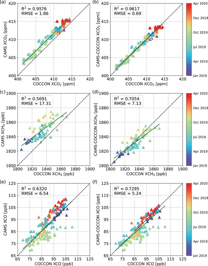
2200                                    C. Alberti et al.: Intercomparison of COCCON and satellite observations in Russia

are only some of the most important causes, which have in-          ing state of the art (Alberti et al., 2021). On that frame-
creased anthropogenic emissions. These activities require the       work, national and international consortiums and agencies
use of huge amounts of energy, among which fossil fuels             have been measuring GHGs in the atmosphere with different
such as coal, oil and natural gas are the main sources since        sampling methods, different spatial resolutions and accura-
the industrial era. Global warming is one of the most dis-          cies. Remote sensing is one of the approaches through which
cussed negative effects caused by the anthropogenic emis-           GHGs can be continuously measured on a global scale.
sions of greenhouse gases (GHGs), mainly carbon dioxide             Such measurements can be made with space-based tech-
(CO2 ), methane (CH4 ) and nitrous oxide (N2 O). These gases        niques by using satellites, like SCanning Imaging Absorp-
absorb part of the infrared emission of the Earth, correspond-      tion spectroMeter for Atmospheric CHartographY (SCIA-
ing to their molecular structure. Consequently, the Earth’s         MACHY), Greenhouse Gases Observing Satellite (GOSAT),
surface temperature increases, resulting in melting of glaciers     Orbiting Carbon Observatory-2 (OCO-2), the Tropospheric
and the Greenland and Antarctic ice sheets, sea level rise,         Monitoring Instrument (TROPOMI) onboard of Sentinel-
droughts, and other negative effects. Global warming leads to       5 Precursor (S5-P), and the Chinese Carbon Dioxide Ob-
a climate change which, in turn, leads to a disruption of the       servation Satellite (TanSat) (Liu et al., 2018). For the val-
hydrological cycle, resulting in unpredictable weather pat-         idation of data products from these spaceborne sensors,
terns (IPCC, 2018, 2021). Therefore, huge efforts are needed        remote-sensing observations are performed by ground-based
on all levels; local, national and global efforts are required in   networks: the Network for the Detection of Atmospheric
order to slow down the GHGs emission tendency. Such ef-             Composition Change (NDACC) with high-resolution Fourier
forts require not only a panel of scientists and engineers but      transform infrared (FTIR) spectrometers network (https://
also politicians, policymakers or decision-makers for imple-        www.ndaccdemo.org/, last access: 11 July 2021) and the
menting effective measures. In that regard, countries have de-      Total Column Carbon Observing Network (TCCON) (http:
bated for more than 3 decades, and such meetings produced           //www.tccon.caltech.edu/, last access: 11 July 2021), which
several important agreements. In 1992, the first global deal        is regarded as the reference network for column GHG
that focused on climate change was created: the UN Frame-           measurements, recently supplemented by the COllaborative
work Convention on Climate Change (UNFCCC), which es-               Column Carbon Observing Network (COCCON) (Frey et
tablished the annual Conference of the Parties (COP). Based         al., 2019). The current constellation of satellites provides
on this meeting, the Kyoto Protocol and the Paris Agreement         highly accurate results with a global coverage; nevertheless,
were created. The Kyoto Protocol began in 2005 and its main         for these and future GHG satellite missions, the aforemen-
aim was committing industrialized economies to reduce the           tioned highly accurate ground-based FTIR measurements are
emission of GHGs for defined and agreed targets. Unfortu-           crucial for their calibration and validation. TCCON was es-
nately, after several years the global anthropogenic emissions      tablished in 2004. However, the expensive instrumentation
of GHGs continued increasing (Harris et al., 2012). The Paris       and required maintenance effort limit the number of sta-
Agreement came into force on November 2016, which aims              tions. Recently, TCCON has been complemented by COC-
to limit global warming below 2 ◦ C or even below 1.5 ◦ C.          CON, which uses low-resolution Bruker EM27/SUN FTIR
Such an objective can only be possible through reducing the         spectrometers (in the following referred to as COCCON in-
GHGs emitted into the atmosphere. Although the majority             strument), developed by Karlsruhe Institute of Technology
of cities have enacted initiatives to measure and control pol-      (KIT) in collaboration with Bruker (Gisi et al., 2012; Hase
lution, the majority of developed interventions are localized       et al., 2016). This instrument is a portable unit and easy to
(Miller et al., 2013; Seinfeld and Pandis, 2016). In general,       operate for non-experts. It has been shown in several peer-
the governments of most countries globally have failed to en-       review studies that COCCON instruments enable users to re-
act effective measures of addressing anthropogenic pollution        trieve GHGs with high precision and accuracy, and several
(Meetham et al., 2016).                                             campaigns have been carried out even at remote sites.
   In summary, we need to know more about the natural                  The EU project VERIFY (https://verify.lsce.ipsl.fr/, last
sources and sinks of GHGs into the atmosphere to better un-         access: 2 July 2021) aims to quantify and estimate the an-
derstand climate change, which will in turn allow for better        thropogenic and natural GHG emissions based on atmo-
projections of their future under climate change conditions.        spheric measurements, emission inventories and ecosystem
Additionally, we need to monitor the anthropogenic emis-            data. Within this project, two cities in Russia (St. Petersburg
sions, e.g. in the context of the Paris Agreement. CO2 , which      and Yekaterinburg) were selected with the objective of im-
is the most important GHG, is long lived as it has an at-           proving our understanding of a key important region with an-
mospheric lifetime which spans from centuries to millennia          ticipated huge biosphere fluxes and potentially extensive car-
(IPCC, 2018).                                                       bon sinks (Reuter et al., 2014). Because only a few measure-
   Both applications require measuring relatively small             ments are available in this region, two different campaigns
changes over a large background concentration, which re-            were carried out there in the framework of VERIFY: con-
quires high accuracy instrumentation and calls for continu-         tinuous measurements at fixed locations in both places and
ous efforts on improving the instrumental and data process-         also a mobile city campaign targeting St Petersburg emis-

Atmos. Meas. Tech., 15, 2199–2229, 2022                                              https://doi.org/10.5194/amt-15-2199-2022
C. Alberti et al.: Intercomparison of COCCON and satellite observations in Russia                                            2201

sions (Emission Monitoring Mobile Experiment, EMME). In         Table 1. ILS in terms of modulation efficiency (M.E.) and phase
the city campaign, two COCCON spectrometers were placed         error calculated before and after the campaign for instruments
upwind and downwind of St Petersburg in 2019. With the          FTS#80 and FTS#84.
obtained results, the emission ratios for the city emissions
were quantified and compared with the bottom-up estima-                 Instrument    Date            M.E.     Phase error
tion as presented in Makarova et al. (2021). From these cam-            FTS#80        17 April 2018   0.9865    −0.00275
paign data, the CO2 , CH4 , NOx and CO fluxes were esti-                              4 June 2020     0.9861    −0.01295
mated as well. Estimation of the anthropogenic CO2 emis-
                                                                        FTS#84        27 March 2018   0.9900    −0.00009
sions using Open-Data Inventory for Anthropogenic Carbon                              4 June 2020     0.9871     0.00083
dioxide (ODIAC) and the FTIR measurements are presented
by Timofeyev et al. (2020), while the CH4 emission inten-
sities are presented by Foka et al. (2020). Additionally, the
EMME campaign was extended in 2020 with only one spec-          2.1     Stability of the COCCON spectrometers during the
trometer moved between the upwind and downwind sides.                   campaign period
The integral CO2 city emission data for both periods are in-
vestigated by Ionov et al. (2021).                              Measurements of very high precision and accuracy are re-
   In contrast to the papers above, this paper focuses on the   quired for correctly retrieving the columnar GHG abun-
complete set of COCCON measurements collected in the            dances in the atmosphere. This can be well achieved with the
framework of VERIFY to validate and compare TROPOMI,            portable FTIR spectrometers as the EM27/SUN spectrom-
OCO-2, GOSAT, MUSICA IASI and Copernicus Atmo-                  eter. To ensure the optimum level of accuracy, prior to the
sphere Monitoring Service (CAMS). Additionally, a scal-         campaign the two instruments were checked, characterized
ing method is developed, and its results are used to bet-       and calibrated, and the residual instrument-specific calibra-
ter inter-compare satellite products. This method is based      tion factors of XCO2 , XCO, XCH4 and XH2 O with respect
on COCCON measurements at both sites to scale CAMS              to the COCCON reference were determined. For demonstrat-
XCO2 , XCH4 and XCO. The effectiveness of this method           ing the stability of the spectrometers, the calibration has been
is proved by using different subsets of XCH4 retrieved from     carried out again after the campaign. This calibration work is
the densest observations from the reference COCCON spec-        described in the next subsections.
trometer (FTS#37) at Karlsruhe during the period of January
2018–December 2020. Because GHGs surface fluxes are im-         2.1.1    Instrumental line shape (ILS) characterization
printed in the atmospheric concentrations, in order to learn
about them it is imperative to accurately estimate their re-    An important step to find any kind of instrumental malfunc-
spective atmospheric gradients. In that regard, the gradients   tion is the laboratory calibration. Open-path measurements
for XCO2 , XCH4 and XCO are calculated between both stud-       described by Frey et al. (2015) and Alberti et al. (2021) were
ied cities during the shared measurement period. Finally, a     performed for recognizing channelling effects, increased
city-scale transport event occurred during the city campaign    noise levels and out-of-band artefacts and for characterizing
and tracked by TROPOMI is presented in this study.              the instrumental line shape (ILS). The ILS for both instru-
                                                                ments was determined at KIT before and after the campaign
                                                                in order to track their stability and thus their performance.
2   Russian campaign location and set-up                        The ILS is given in terms of modulation efficiency (M.E.)
                                                                and phase error (Table 1).
Within the VERIFY project, two cities in Russia (St Peters-
burg and Yekaterinburg) were chosen as target regions. The
                                                                2.1.2    Side-by-side measurements
main aim was to collect observations for evaluating XCO2
gradients and the XCO/XCO2 ratios in a very important re-
                                                                After the instruments were calibrated, solar side-by-side
gion with high emissions and large biosphere fluxes in east-
                                                                measurements between the instruments used in the cam-
ern Europe. To achieve the foreseen objectives two differ-
                                                                paign (FTS#80 and FTS#84), the COCCON reference and
ent activities were carried out: a mobile city campaign (see
                                                                the TCCON spectrometer operated at the same location were
Sect. 2.2) and continuous measurements in two fixed loca-
                                                                carried out at KIT. These measurements served to find the
tions: Peterhof (15 months) and Yekaterinburg (6 months)
                                                                instrument-specific calibration factors for each retrieved gas.
(see Sect. 2.3).
                                                                These factors are calculated with respect to the COCCON
                                                                reference and help to harmonize the results for all COCCON
                                                                spectrometers. Such measurements took place before (18 and
                                                                19 April 2018) and during (12 April 2019) the campaign. The
                                                                later one served for crosschecking whether the instruments
                                                                kept the same behaviour and performance. These results can

https://doi.org/10.5194/amt-15-2199-2022                                             Atmos. Meas. Tech., 15, 2199–2229, 2022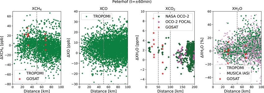
2202                                   C. Alberti et al.: Intercomparison of COCCON and satellite observations in Russia

be seen in Figs. 1 and 2, respectively, and the correction fac-   Peterhof was operated by the Russian partners at the At-
tors are listed in Table 2.                                       mospheric Physics Department of the Faculty of Physics at
   From the measurements shown in Fig. 1, the correction          Saint Petersburg State University. The instrument was set up
factors for XCO2 , XCO and XCH4 measured by the two in-           on every sunny day (outside the city campaign period) at the
struments are calculated as described in Frey et al. (2019)       second floor of the FTIR remote-sensing group (see Fig. 4).
and Alberti et al. (2021). These results are averaged and later   Eighty-four measurement days were collected between Jan-
used for scaling the results for each of the retrieved GHGs       uary 2019 and March 2020 as can be seen in Fig. 5. From that
analysed in this study as presented in Table 2.                   figure, the larger XCO observed values on 6 August 2019 in
                                                                  comparison to all the other days is remarkable. For more de-
2.2     EMME campaign                                             tails, see Fig. A1a and b, where the spatial distribution of
                                                                  TROPOMI XCH4 and XCO, as well as wind speed and di-
The EMME campaign is described in detail by Makarova              rection, respectively, for this day are presented. Additionally
et al. (2021), and here we summarize only the most rele-          Fig. A1c shows the time series for COCCON XCO2 , XCH4
vant details of it. Because the aim of this campaign was to       and XCO for that day, and the enhancements are all observed
quantify the CO2 emissions; CO/CO2 emission ratios; and           in the three species. It seems that these large values could
the estimation of the CO2 , CH4 , and CO fluxes, two mo-          be related to a plume transport from a heavily industrial-
bile COCCON FTIR spectrometers were used in order to              ized area coming from Lappeenranta, which is located in the
retrieve the required GHG species. Both instruments were          southeast of Finland and approximately 160 km away from
located in the upwind and downwind regions of the St Pe-          Peterhof (see Fig. A2a). In order to confirm this, Fig. A2a
tersburg city ring. This campaign was not made in a con-          shows the yearly CO emissions coming from the “Combus-
tinuous acquisition mode, but the active phases were sched-       tion from manufacturing sector” taken from the EDGAR V05
uled according to the weather forecast. The basic idea is         inventory (latest available: 2015), together with the backward
to select the deployment position of each instrument a day        trajectories calculated by using the HYSPLIT model and ar-
before good meteorological conditions appeared. The wind          rived in Peterhof on that day (see Fig. A2b). This confirms
forecast, and the orientation of the city’s NO2 plume as mod-     that the wind comes from the area where huge anthropogenic
elled by HYSPLIT (HYbrid Single-Particle Lagrangian Inte-         CO sources are located. Another possibility could be an even
grated Trajectory) (https://www.ready.noaa.gov/HYSPLIT_           closer local source, like a small fire.
traj.php, last access: 4 August 2021) were used as predic-
tion tools, and the positions of the COCCON spectrometers         2.3.2   Yekaterinburg (56.8◦ N, 60.6◦ E)
were selected accordingly. In addition, during a measuring
day, the Russian partners carried out mobile zenith DOAS          It was planned that immediately after the EMME campaign
(differential optical absorption spectroscopy) measurements       the instrument FTS#84 would be transported to Yekaterin-
in order to measure the NO2 total column flux over the city in    burg. Unfortunately, unforeseen organizational problems sig-
a near-real time manner. The second input helped to readjust      nificantly delayed moving the instrument from St. Petersburg
the location of one or both spectrometers in case of devi-        to Yekaterinburg. The instrument was finally operational in
ations from the predicted plume orientation. Following this       Yekaterinburg in October 2019 and kept measuring until the
approach, a total of 11 successful measurement days were          very last day before being shipped back to KIT (April 2020).
carried out during March to April 2019. An overview of the        The instrument was operated at the Climate and Environmen-
collected COCCON data is presented in Fig. 3; from that fig-      tal Physics Laboratory INSMA of the Ural Federal Univer-
ure the enhancement on 25 April 2019 is remarkable. This          sity (UrFU). The instrument was set up in an internal yard
measurement day is presented as a plume transport event in        of the UrFU building. However, the building structure, which
a city-scale domain tracked by TROPOMI as a complement            blocked the sunlight, was a limitation. Sometimes high trucks
of the results shown by Makarova et al. (2021).                   passing through the yard blocked the field of view of the in-
                                                                  strument (see Fig. 6). The spectrometer rested on the win-
2.3     Ground-based FTIR measurements at Peterhof                dowsill of the basement, so it was located exactly at ground
        and Yekaterinburg                                         level ∼ 260 m. Under good weather conditions, measure-
                                                                  ments were carried out approximately between 11:00 and
For the continuous, long-baseline campaign, the instrument        14:30 LT. In total, 22 d of measurements were collected as
FTS#80 remained at Peterhof station at the Saint Petersburg       can be seen in Fig. 7.
State University and continued operation there, while the
other spectrometer (FTS#84) was moved to Yekaterinburg.

2.3.1    Peterhof (59.88◦ N, 29.83◦ E)

Peterhof is a suburb of St. Petersburg located approximately
35 km southwest from the city centre. The instrument in

Atmos. Meas. Tech., 15, 2199–2229, 2022                                            https://doi.org/10.5194/amt-15-2199-2022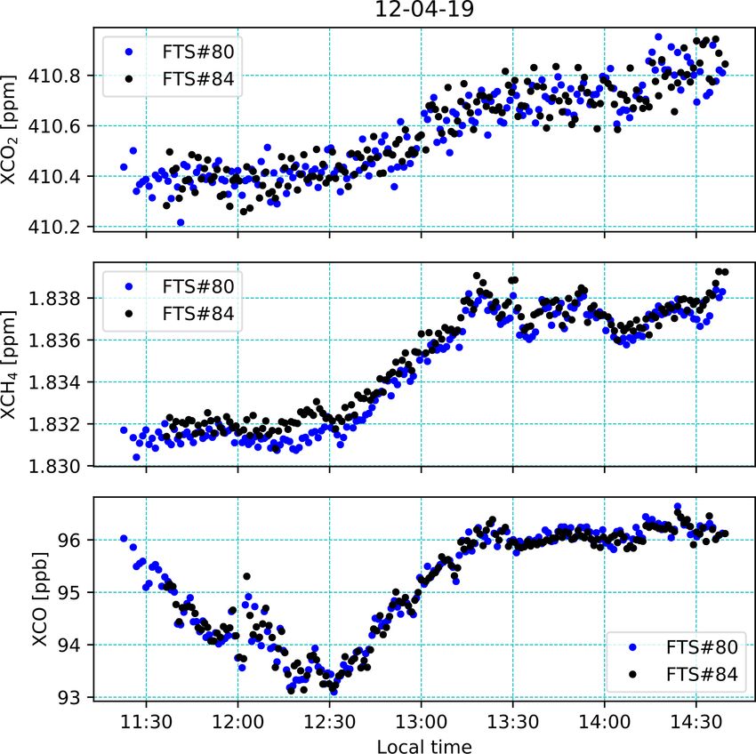
C. Alberti et al.: Intercomparison of COCCON and satellite observations in Russia                                                  2203

Figure 1. Side-by-side measurements before the instruments were shipped to Russia. Comparisons between instrument no. 1 (FTS#37),
which is the COCCON reference unit operated at KIT, and instruments FTS#80 and FTS#84.

Table 2. Correction factors for instruments FTS#80 and FTS#84. The italicized values show the small drift of the instruments and the used
values on the analysis.

                           Instrument    Date                  XCO2 factor     XCH4 factor       XCO factor
                           FTS#80        18–19 April 2018          0.99988          1.00013         1.00636
                                         31 October 2020           0.99981          1.00042         1.00264
                                         Absolute drift       6.765 × 10⁻⁵     2.966 × 10⁻⁴    3.721 × 10⁻³
                                         Used value                0.99984          1.00028         1.00450
                           FTS#84        18–19 April 2018          0.99990          0.99987         1.00748
                                         13 June 2021              0.99967          0.99953         1.00171
                                         Absolute drift       2.242 × 10⁻⁴     3.333 × 10⁻⁴    5.774 × 10⁻³
                                         Used value                0.99978          0.99970         1.00460

3     Datasets                                                         erated by different research groups. It has been shown in
                                                                       several studies that the results for these GHGs observed by
In the following subsections, all the datasets used for this           COCCON instruments are in good agreement with official
study are summarized, and a quick overview of them can be              TCCON results (Frey et al., 2021; Sha et al., 2020). With
found in Table A1 in Appendix A.                                       the characteristics of compactness, robustness and portabil-
                                                                       ity, these instruments have been successfully used in sev-
3.1    Ground-based data                                               eral field campaigns and continuous deployments (Hase et
                                                                       al., 2015; Klappenbach et al., 2015; Chen et al., 2016; Butz et
COCCON
                                                                       al., 2017; Sha et al., 2020; Vogel et al., 2019; Tu et al., 2020,
Recently, COCCON (https://www.imk-asf.kit.edu/english/                 2021, 2022; Jacobs et al., 2020; Frey et al., 2021; Dietrich
COCCON.php, last access: 13 May 2021; Frey et al., 2019)               et al., 2021; Jones et al., 2021). A preprocessing tool and
was established by continuous support granted by the Euro-             the PROFFAST non-linear least squares fitting algorithm are
pean Space Agency (ESA). COCCON provides a supporting                  used for data retrieval. This processing software was created
infrastructure for GHG measurements using the EM27/SUN                 in the framework of the ESA COCCON-PROCEEDS and
spectrometer and ensures common standards for instrumen-               COCCON-PROCEEDS II projects. The solar zenith angle
tal quality management and data analysis. The EM27/SUN                 (SZA) range of COCCON data used in this study is restricted
spectrometer was developed by KIT in cooperation with the              to ≤ 70◦ in order to limit uncertainties connected with spec-
Bruker company in 2011 (Gisi et al., 2012). A second detec-            tra recorded at very high air masses.
tor channel for XCO observations was added in 2015 (Hase
et al., 2016). The EM27/SUN spectrometers are widely used,
and there are currently about 78 instruments globally op-

https://doi.org/10.5194/amt-15-2199-2022                                                 Atmos. Meas. Tech., 15, 2199–2229, 2022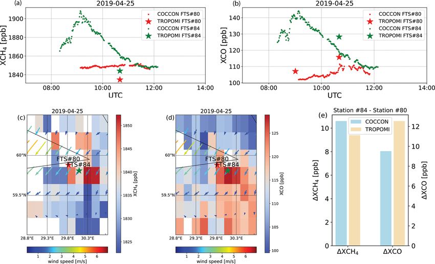
2204                                   C. Alberti et al.: Intercomparison of COCCON and satellite observations in Russia

                                                                   3.2.2   OCO-2

                                                                   The Orbiting Carbon Observatory-2 (OCO-2) is a NASA
                                                                   satellite, launched in July 2014, providing space-based mea-
                                                                   surements of atmospheric CO2 (Eldering et al., 2017). These
                                                                   observations have the potential capability to detect CO2
                                                                   sources and sinks with unprecedented spatial and tempo-
                                                                   ral coverage and resolution (Crisp, 2015). The OCO-2 mis-
                                                                   sion carries a single instrument incorporated with three high-
                                                                   resolution imaging grating spectrometers, collecting spectra
                                                                   from reflected sunlight by the surface of Earth in the molec-
                                                                   ular oxygen (O2 ) A band at 0.764 µm and two CO2 bands at
                                                                   1.61 and 2.06 µm (Osterman et al., 2020). The OCO-2 satel-
                                                                   lite has three viewing modes (nadir, glint and target) and a
                                                                   near-repeat cycle of 16 d (98.8 min per orbit, 233 orbits in
                                                                   total). It samples at a local time of about 13:30 LT. The cur-
                                                                   rent version (V10r) of the OCO-2 Level 2 (L2) data product,
                                                                   containing bias-corrected XCO2 , is used in this study.
                                                                      In addition to the operational XCO2 product derived from
                                                                   OCO-2 observations described above, the data product gen-
                                                                   erated using the Fast atmOspheric traCe gAs retrievaL (FO-
Figure 2. Side-by-side measurements during the campaign but only   CAL) algorithm described in Reuter et al. (2017a, b) had
with instruments FTS#80 and FTS#84.                                been used. Compared with co-located TCCON observa-
                                                                   tions, the OCO-2 FOCAL data show a regional-scale bias of
                                                                   about 0.6 ppm and single measurement precision of 1.5 ppm
3.2     Spaceborne data                                            (Reuter and Buchwitz, 2021). In this study, the latest version
                                                                   (v09) covering the time period of 2015–2020 is utilized for
3.2.1    TROPOMI                                                   further comparison with the COCCON results.

The Sentinel-5 Precursor (S5-P) satellite with the Tropo-          3.2.3   MUSICA IASI
spheric Monitoring Instrument (TROPOMI) on board as a
single payload was launched in October 2017. S5-P is a low-        The Infrared Atmospheric Sounding Interferometer (IASI) is
Earth-orbit polar satellite. It aims at monitoring air quality,    a payload on board the EMETSAT Metop series of polar-
climate and ozone layer with high spatio-temporal resolu-          orbiting satellites (Clerbaux et al., 2009). The IASI instru-
tion and daily global coverage during an operational lifes-        ment is a Fourier transform spectrometer that measures in-
pan of 7 years (Veefkind et al., 2012). TROPOMI is a               frared radiation emitted from the Earth and emitted and ab-
nadir-viewing grating-based imaging spectrometer, measur-          sorbed by the atmosphere. It provides unprecedented accu-
ing backscattered solar radiation spectra with an unprece-         racy and resolution on atmospheric humidity profile, as well
dented resolution of 7 × 7 km2 (upgraded to 5.5 × 7 km2 in         as total column-integrated CO, CH4 and other compounds
August 2019; Lorente et al., 2021b). In this study, we use         twice a day. There are currently three IASI instruments in
the improved TROPOMI XCH4 product derived with the Re-             operation on Metop-A, Metop-B and Metop-C, launched in
moTeC full-physics algorithm (Lorente et al., 2021b) and ap-       2006, 2012 and 2018, respectively. The MUSICA IASI re-
ply the recommended quality value (qa) = 1.0 to the data.          trievals are based on a nadir version of PROFFIT (Schneider
For CO, SICOR (Shortwave Infrared CO Retrieval algo-               and Hase, 2009), which has been developed in support of the
rithm) is deployed to retrieve the total column density of CO      MUSICA project. More details can be found in Schneider
from TROPOMI spectra at 2.3 µm (Landgraf et al., 2016;             and Hase (2011) and Schneider et al. (2022). A validation of
Borsdorff et al., 2018a, b). XCO is computed by divid-             the MUSICA IASI H2 O profile data is presented by Borger
ing the CO total column by the dry air column extracted            et al. (2018).
from the co-located TROPOMI CH4 file. This dry air col-
umn is obtained from the surface pressure and water vapour         3.2.4   GOSAT
column as provided by the European Centre for Medium-
Range Weather Forecasts (ECMWF) analysis (Schneising et            The Greenhouse Gases Observing Satellite (GOSAT) was
al., 2019; Lorente et al., 2021b). H2 O retrievals are also per-   launched in January 2009, equipped with two instruments
formed with the SICOR algorithm. A similar quality filter is       (the Thermal And Near-infrared Sensor for carbon Observa-
applied to the H2 O product as used in Schneider et al. (2020).    tion Fourier Transform Spectrometer, TANSO-FTS, and the

Atmos. Meas. Tech., 15, 2199–2229, 2022                                             https://doi.org/10.5194/amt-15-2199-2022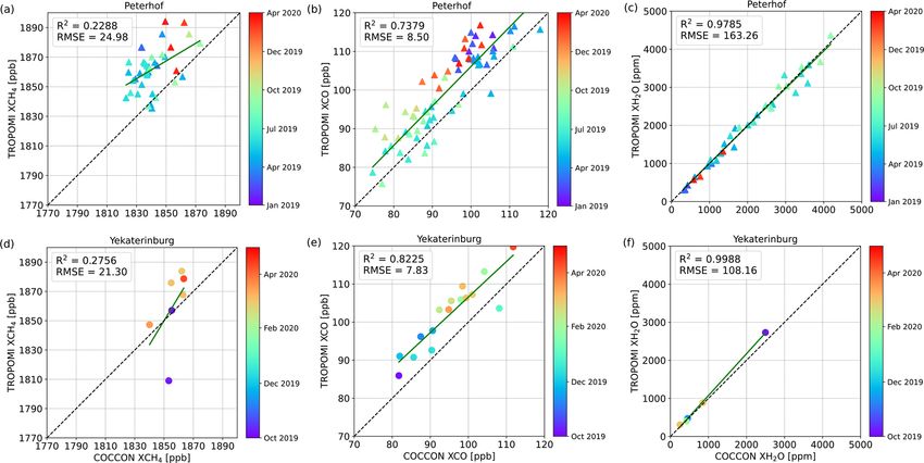
C. Alberti et al.: Intercomparison of COCCON and satellite observations in Russia                                            2205

Figure 3. General overview of the full campaign results collected with the COCCON spectrometers (Makarova et al., 2021).

                                                                      3.3     CAMS data

                                                                      3.3.1    CAMS inversion

                                                                      Copernicus Atmosphere Monitoring Service (CAMS) is op-
                                                                      erated by the European Centre for Medium-Range Weather
                                                                      Forecasts (ECMWF), providing global inversion-optimized
                                                                      GHG concentration products which are updated once or
                                                                      twice per year. For XCO2 and XCH4 , the latest version
                                                                      datasets (v20r1 for XCO2 and v19r1 for XCH4 ) using surface
                                                                      air-sample as observations input are used in this study. The
                                                                      CAMS global CO2 atmospheric inversion product is gener-
                                                                      ated by the inversion system, called PyVAR (Python VARi-
                                                                      ational), with a horizontal resolution of 1.875◦ × 3.75◦ and
                                                                      temporal resolution of 3 h (Chevallier, 2020a, b). The lat-
                                                                      est version (V20r1) was released in December 2020, cover-
                                                                      ing the period from January 1979 to May 2020. The V20r1
                                                                      model data fit TCCON retrievals well with less than 1 ppm
                                                                      of absolute biases (Chevallier, 2020b).
                                                                         For XCH4 , we used the latest version V19r1 based on
                                                                      inversion of surface observations only, covering the period
                                                                      between January 1990 and December 2019. The CAMS
                                                                      XCH4 inversion product is based on the TM5-4DVAR (four-
Figure 4. Instrument set-up at Peterhof. A huge window allowed for    dimensional variational) inverse modelling system (Bergam-
measurements from ∼ 10:00 to ∼ 15:30 LT (local time) every day.       aschi et al., 2010, 2013; Meirink et al., 2008) with a hori-
                                                                      zontal resolution of 2◦ × 3◦ and temporal resolution of 6 h
                                                                      (Segers, 2020a, b). Compared to previous releases, v19r1
TANSO Cloud and Aerosol Imager, TANSO-CAI) (Kuze et
                                                                      data have been adjusted by using new atmospheric CH4
al., 2009). The satellite is placed on a Sun-synchronous or-
                                                                      sinks and updated wetland emissions, and the monthly bias
bit and passes the same point on Earth every 3 d. GOSAT is
                                                                      is usually less than 10 ppb with respect to TCCON (Segers,
the first mission to monitor the global distribution and sinks
                                                                      2020b).
and sources of GHGs. For this study, GOSAT FTS shortwave
infrared (SWIR) level-2 data, version V02.90, from the Na-
                                                                      3.3.2    CAMS reanalysis (control run)
tional Institute for Environmental Studies (NIES) are used.
                                                                      This study aims to compare XCO retrieved from the COC-
                                                                      CON measurements with XCO from different satellite and
                                                                      CAMS datasets as well. However, no XCO data are avail-
                                                                      able from the before-mentioned CAMS data. Fortunately,

https://doi.org/10.5194/amt-15-2199-2022                                                Atmos. Meas. Tech., 15, 2199–2229, 2022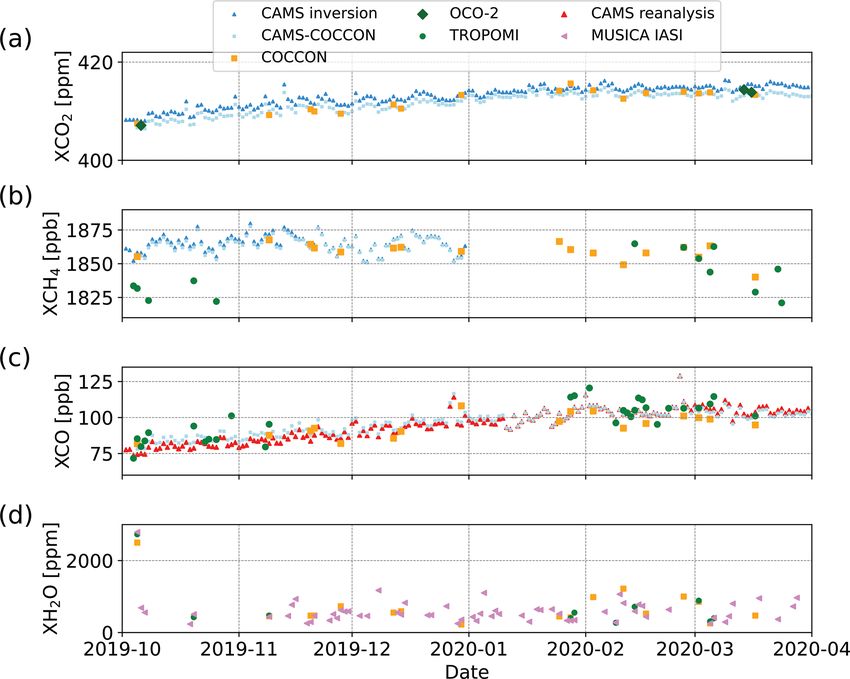
2206 C. Alberti et al.: Intercomparison of COCCON and satellite observations in Russia
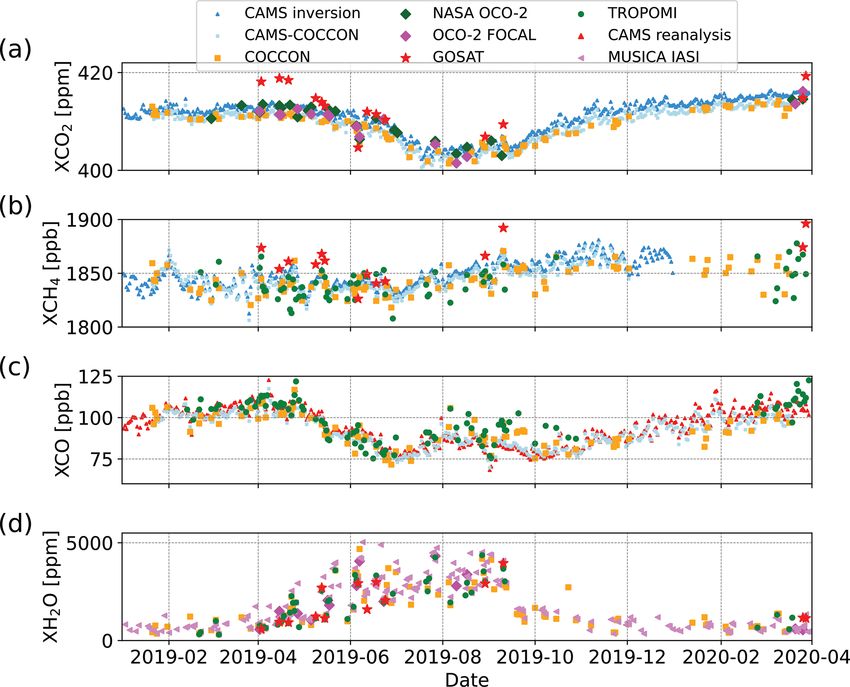
Figure 5. Time series for XCO2 , XCO and XCH4 obtained in Peterhof during the continuous campaign.
XCH4 , XCO and XH2 O from different data products at
Peterhof. The CAMS-COCCON data product presented in
Figs. 8 and 9 is discussed in Sect. 4.3. The TROPOMI satel-
lite has a higher spatial resolution and therefore, the avail-
able retrieved species from TROPOMI were daily averaged
within a collection radius of 50 km around Peterhof. For the
GOSAT and MUSICA IASI datasets, a collection radius of
100 km around Peterhof is used, and for OCO-2 data, a col-
lection radius of 200 km is used. The choice of collecting
radius is considered based on the available satellite obser-
vations and the bias between a single satellite observation
and the coincident COCCON observation (see Fig. A3). The
measurements from the different ground- and space-based
observations and model data generally show good agree-
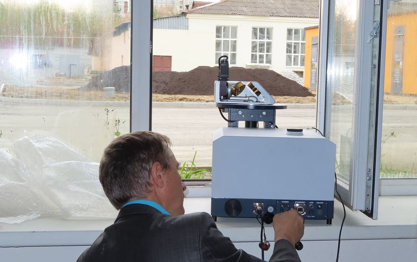
Figure 6. Instrument set-up at Yekaterinburg. The time interval of ments and similar seasonal variability.
the daily measurements was constrained by the building structure,
CAMS and the satellite products show a high bias of about
which blocked the sunlight.
0.81 to −3.1 with respect to COCCON. GOSAT (Fig. 8a)
also shows some obvious outliers compared to the other
products, which have similar behaviours. The amount of
CAMS also provides reanalysis datasets, covering the pe-
XCO2 varies along the year, and much of this variation is
riod of 2003–June 2020. The standard CAMS reanalysis data
driven by respiration, which never stops but increases be-
use 4DVar data assimilation in CY42R1 of ECMWF’s Inte-
tween autumn and winter due to reduced uptake (no photo-
grated Forecast System (IFS) (Flemming et al., 2017; Inness
synthesis). In this case the atmospheric XCO2 concentration
et al., 2019). The CAMS reanalysis CO profiles under a con-
is stable between January and April. It started to decrease
trol run, i.e. without any data assimilation, is obtained from
from May to end of July, during which the growing season
Copernicus Support team. This control run reanalysis CO
and the photosynthetic activities increase. Similar behaviour
profiles are using only one IFS cycle with a 0.1◦ × 0.1◦ lat-
in 2019 was also observed by Timofeyev et al. (2021) and in
itude × longitude resolution, 3 h of temporal resolution and
previous years by Timofeyev et al. (2019) and Nikitenko et
25 pressure levels. XCO is obtained when integrating the pro-
al. (2020). The amount of XCO2 stays around 403 ppm be-
files from the lowest to the highest pressure level.
tween the end of July and middle of September and starts to
increase afterwards.
4 Results and discussion For XCH4 , COCCON shows a similar behaviour as
TROPOMI and CAMS. Slightly higher mean values and
4.1 Seasonal variability of GHGs variability can be seen in GOSAT XCH4 with a few outliers.
Compared to XCO2 , XCH4 shows generally less seasonal
4.1.1 Peterhof variabilities with more short-term enhancements of about a
week duration, probably related to synoptic variations. The
The seasonal patterns of the retrieved GHGs are shown in seasonal variation is comparable to the results of Gavrilov
Fig. 8, which illustrates the time series of daily mean XCO2 ,
Atmos. Meas. Tech., 15, 2199–2229, 2022 https://doi.org/10.5194/amt-15-2199-2022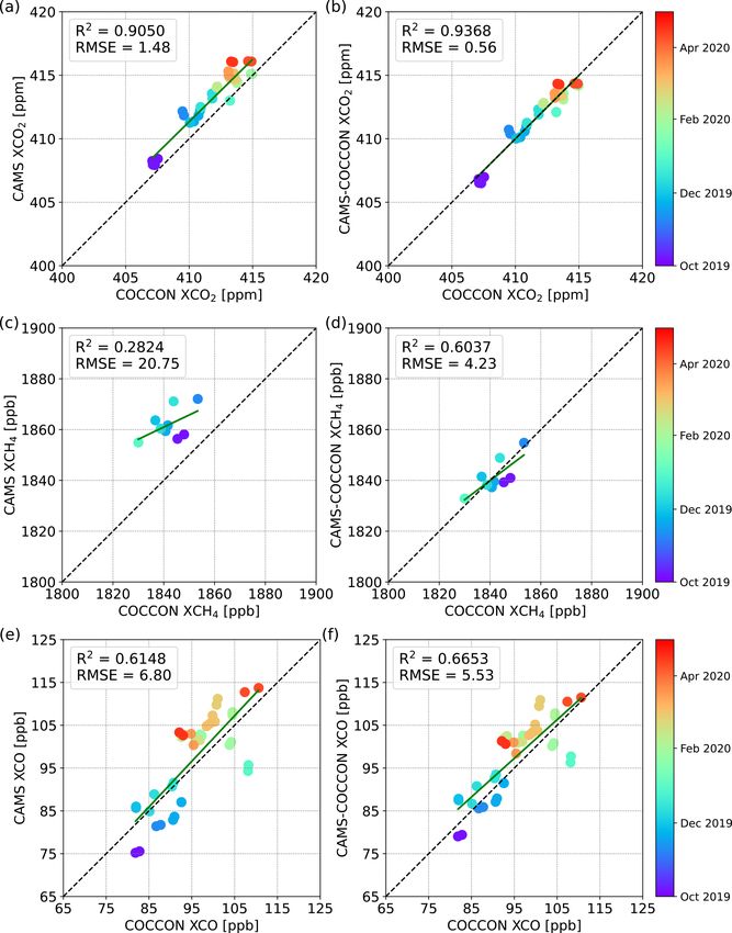
C. Alberti et al.: Intercomparison of COCCON and satellite observations in Russia                                          2207

Figure 7. Time series of XCO2 , XCO and XCH4 data observed at Yekaterinburg.

et al. (2014), Makarova et al. (2015a, b) and Timofeyev et            XCO2 shows a clearly increasing tendency from Octo-
al. (2016). A slightly higher XCH4 is observed at the end of       ber of 408 ppm to a maximal value of 415 ppm in the
2019 for all data products.                                        middle of February, which covers later autumn and win-
   XCO shows seasonal variability with a maximal value of          ter. This is because on top of the increase due to the
110 ppb in late April and decreases by nearly 40 % to 70 ppb       anthropogenic emissions there are variations due to pho-
in the beginning of July. A secondary local maximal reach-         tosynthesis and respiration (https://atmosphere.copernicus.
ing ∼ 95 ppb occurs in August. This feature needs further in-      eu/carbon-dioxide-levels-are-rising-it-really-simple, last ac-
vestigation. The COCCON XCO matches well to the CAMS               cess: 2 July 2021). During that period the plants notably re-
reanalysis data. Moreover, COCCON agrees better with the           duce or stop the photosynthesis processes which could in-
TROPOMI data in summer than in spring and late autumn,             crease the amount of CO2 in the atmosphere. Later this max-
when TROPOMI measured higher values.                               imal value stays constant until the middle of March. It tends
   XH2 O shows a strong seasonal cycle with a maximal              to decrease, and a similar behaviour is observed in Peterhof.
amount of ∼ 4700 ppm in summer and minimal amount of                  For XCH4 , COCCON shows a good agreement with
∼ 320 ppm in winter. All products show quite similar be-           CAMS data, though there are not so many COCCON ob-
haviour with high variability, which is similar to those in Se-    servations. XCH4 shows generally decreasing tendency but
menov et al. (2015), Timofeyev et al. (2016) and Virolainen        with more short-term variabilities. Such variabilities are ob-
et al. (2016, 2017). The GOSAT data have higher mean val-          served in Peterhof as well. A few TROPOMI observations
ues since the measurement period covers only the time range        in October are deviating from the other two datasets, and it
from later spring to summer, during which higher XH2 O is          seems that TROPOMI underestimates XCH4 . This might be
observed.                                                          because most TROPOMI measurements are located in the
                                                                   rim of the collecting radius and thus away from the loca-
                                                                   tion of Yekaterinburg, introducing some errors (see Fig. A5).
4.1.2   Yekaterinburg                                              Further, this underestimation could be due to the difficulty
                                                                   for retrieving CH4 in low- and high-albedo scenes (Lorente
                                                                   et al., 2021b).
The measurement period covered winter and spring, from
                                                                      XCO shows in general a similar behaviour of XCO2 , with
5 October 2019 to 17 April 2020 at Yekaterinburg (Fig. 9).
                                                                   a steady increase during late autumn and winter. It seems that
Here we use a larger radius (100 km) to collect the
                                                                   the increasing behaviour of XCO has an inverse relationship
TROPOMI observations, because there are much fewer over-
                                                                   with XCH4 . This is probably due to the fact that atmospheric
passes at Yekaterinburg during this period. Table A2 in Ap-
                                                                   CO is mainly produced by incomplete combustion of fossil
pendix A lists the number of coincidences (pixel-wise) for
                                                                   fuels (Kasischke and Bruhwiler, 2002) and the oxidation of
50 and 100 km radius, and the number of coincident satel-
                                                                   methane (Cullis and Willatt, 1983).
lite pixels is reduced by a factor of 3 to 5 for the narrower
                                                                      As expected, most XH2 O values are below 1000 ppm, sim-
radius. From Fig. A4 in Appendix A, we do see a tendency
                                                                   ilar to Peterhof in that period. This can be explained by the
of slightly reduced differences with better co-location within
                                                                   saturation concentration of water vapour in air, which re-
the 100 km limit in case of XCH4 but not clearly for the other
                                                                   duces for lower temperatures.
species. Due to the low number of coincident measurements
when using 50 km, we decided to accept the 100 km distance
criterion for the Yekaterinburg observations.

https://doi.org/10.5194/amt-15-2199-2022                                            Atmos. Meas. Tech., 15, 2199–2229, 2022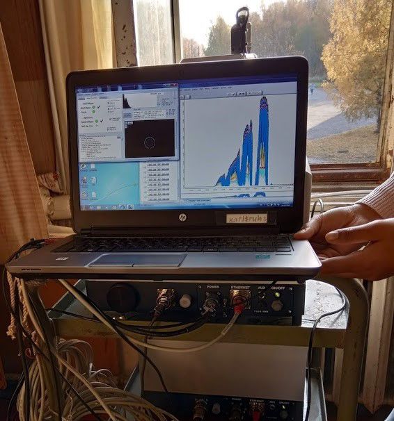
2208                                     C. Alberti et al.: Intercomparison of COCCON and satellite observations in Russia

Figure 8. Time series of daily mean (a) XCO2 , (b) XCH4 , (c) XCO and (d) XH2 O for different data products at Peterhof.

Figure 9. Time series of daily mean (a) XCO2 , (b) XCH4 , (c) XCO and (d) XH2 O for different data products at Yekaterinburg.

Atmos. Meas. Tech., 15, 2199–2229, 2022                                                  https://doi.org/10.5194/amt-15-2199-2022
C. Alberti et al.: Intercomparison of COCCON and satellite observations in Russia                                                  2209

4.2    Removal of the smoothing error bias                               which turns into

Because we aim at comparing different data products (such                Xgas, obs−new

as spaceborne and COCCON products) and each of them                        = Xgas, obs−sat + Xgas, apr−new − Xgas, apr−sat
use different sensitivities and different a priori profiles, it is           Xk
important to account for these differences when comparing                  +   0
                                                                                 h k ak VMR  apr−sat,k − VMR  apr−new,k    ,         (4)
a defined Xgas species as described by Rodgers and Con-
                                                                         where Xgas, obs−new in Eq. (4) becomes the smoothed satellite
nor (2003) and Connor et al. (2008). Such procedures have
                                                                         product, which takes into account the a priori profiles used
been applied in similar studies (Hedelius et al., 2016; Yang et
                                                                         for the COCCON retrievals.
al., 2020; Sha et al., 2021). In this study, we used the method
                                                                            When using Eq. (4), both a priori profiles need to be re-
described in Connor et al. (2008). We took as starting point
                                                                         sampled on the same pressure grid. The vertical profiles used
their Eq. (13); then the state vector can be written as
                                                                         for the COCCON analysis are interpolated to the pressure

V MR gas, obs = V MR gas, apr + A V MR true − V MR gas, apr ,      (1)   levels of different satellite products (TROPOMI CO, GOSAT
                                                                         CO2 and CH4 , OCO-2 CO2 , and OCO-2 FOCAL CO2 ) by
where VMR represents the volume mixing ratio. The left-
                                                                         using the mass conservation method described in Langerock
hand term of the equation represent the retrieved value, while
                                                                         et al. (2015).
the right-hand term represents the VMR calculated based on
                                                                            The smoothing correction is not applied to XH2 O, because
the a priori profiles plus the effect of the averaging kernel
                                                                         the natural variability of XH2 O is very high anyway.
matrix A applied to the difference of the VMR between the
true atmospheric gas concentration and the a priori profiles.            4.3   Correlation between COCCON and satellite
By dividing the atmosphere into k layers, this equation can                    products
be written as follows:
                               k
                               X                                         All satellite XCO2 , XCH4 and XCO data used in this sec-
                                                                         tion were adjusted for the COCCON a priori profile (TCCON

Xgas, obs = Xgas, apr +             hk ak VMRtrue,k − VMRapr,k ,
                                0                                        a priori profiles were used) as described above. In addition, in
                                                                   (2)   the Supplement of this paper, the comparisons with the orig-
                  P                                                      inal COCCON products (see Figs. S1 to S4 in the Supple-
where Xgas,y =         hk ·VMRy,k with y being a defined a priori        ment) and without taking into account the averaging kernels
                   k
profile used and hk being the pressure-weighting function in             when comparing with satellite products are presented.
a defined layer k (Connor et al., 2008), i.e.                               Figures 10 to 13 show the correlations between COCCON
                                                                         and different satellite products at Peterhof (triangle symbols)
       (pk−1 − pk )
hk =                .                                              (3)   and at Yekaterinburg (dot symbols). The satellite products
           p0                                                            and CAMS generally agree well with COCCON. Figure 14
By using Eq. (2) with “new” and “old” satellite a priori pro-            illustrates the averaged bias and standard deviation of each
files, we obtain (∗ ) and (∗∗ ) as follows:                              product of the coincident Xgas (XCO2 , XCH4 and XCO) val-
 Xgas, obs−new = Xgas, apr−new                                           ues (in space-time) with respect to COCCON for the avail-
                 k                                                       able gases at both sites. In order to find the coincident COC-
              + hk ak VMRtrue,k − VMRapr−new,k (∗ )
                P
                                                                         CON data, the mean value of the observations 2 h before and
                   0                                                     after a centralized time reference is taken. Such a time refer-
 Xgas, obs−sat = Xgas, apr−sat                                           ence differs for each of the products as follows: the overpass
                  k
                                                                (∗∗ ).   time for satellite and each of the timestamps for CAMS.
                  P
                + hk ak VMRtrue,k − VMRapr−sat,k
                       0                                                    The measuring period at Yekaterinburg for COCCON was
Then we subtract (∗ ) from (∗∗ ):                                        mostly in winter and early spring, from October 2019 to
                                                                        April 2020, in which there were fewer sunny days. This re-
Xgas, obs−new = Xgas, obs−sat + Xgas, apr−new − Xgas, apr−sat            sults in fewer COCCON and satellite observations. There is
                       k
                       X                                                 only one coincident point between COCCON and NASA op-
                 +             hk ak VMRtrue,k                           erational OCO-2 (Fig. 11c) and no coincident points between
                       0                                                 COCCON and OCO-2 FOCAL or GOSAT products at Yeka-
                       k
                       X                                                 terinburg. Even a much larger collection circle with a radius
                 −             hk ak VMRapr−new,k                        of 100 km is used for TROPOMI at Yekaterinburg, and there
                       0                                                 are fewer coincidence measurements than those in Peterhof,
                       k
                       X                                                 where more than 1 year of measurements were performed.
                 −             hk ak VMRtrue,k                              Due to the short period of ground-based measurements,
                           0
                       Xk                                                poor weather condition, and poorer coverage of satel-
                 +              h a VMRapr−sat,k ,
                               0 k k
                                                                         lites at high latitudes in the winter hemisphere (OCO-

https://doi.org/10.5194/amt-15-2199-2022                                                    Atmos. Meas. Tech., 15, 2199–2229, 2022
2210 C. Alberti et al.: Intercomparison of COCCON and satellite observations in Russia
Figure 10. Correlation plots between TROPOMI and COCCON for XCH4 , XCO and XH2 O at Peterhof (a–c) and at Yekaterinburg (d–f).
All satellite data except XH2 O were adjusted for the COCCON a priori profile (TCCON a priori profiles were used).
Figure 11. Correlation plots (a–b) between NASA’s operational and the FOCAL OCO-2 product and COCCON for XCO2 and (c) between
OCO-2 FOCAL and COCCON for XH2 O at Peterhof. All satellite data except XH2 O were adjusted for the COCCON a priori profile
(TCCON a priori profiles were used).
2; Patra et al., 2017, and GOSAT; https://data2.gosat.nies. TROPOMI XCO shows higher biases than CAMS with re-
go.jp/gallery/fts_l2_swir_co2_gallery_en.html, last access: spect to COCCON, which can be seen in Figs. 8c and 9c
28 June, 2021), it becomes more difficult to validate satel- – TROPOMI with higher values than COCCON. TROPOMI
lite products with ground-based measurements at locations and GOSAT generally measure lower XH2 O than COCCON,
like Yekaterinburg. whereas MUSICA IASI shows high bias and standard devia-
At Peterhof OCO-2 FOCAL XCO2 data have the low- tion. However, good correlations can be found between satel-
est bias with respect to COCCON, while GOSAT data show lite XH2 O and COCCON in Figs. 10c, f, 12c and 13.
the highest bias and standard deviation (3.6 ppm ± 2.8 ppm,
Fig. 14). NASA operational OCO-2 and CAMS show simi- 4.4 Using CAMS model fields for upscaling COCCON
lar biases. CAMS, TROPOMI and GOSAT measure higher observations
XCH4 than COCCON, among which GOSAT has the high-
est biases at Peterhof. The high negative bias in TROPOMI Unfortunately, during the continuous campaign carried out
at Yekaterinburg is mainly due to the underestimation of at Peterhof and Yekaterinburg, there are just a few coincident
the TROPOMI product in October 2019. At both sites measurement days with satellite observations, especially in
comparison to GOSAT and OCO-2 (see Fig. 14). Although
Atmos. Meas. Tech., 15, 2199–2229, 2022 https://doi.org/10.5194/amt-15-2199-2022C. Alberti et al.: Intercomparison of COCCON and satellite observations in Russia 2211 Figure 12. Correlation plots between GOSAT and COCCON for (a) XCH4 , (b) XCO and (c) XH2 O at Peterhof. All satellite data except XH2 O were adjusted for the COCCON a priori profile (TCCON a priori profiles were used). Figure 13. Correlation plots of XH2 O between MUSICA IASI and COCCON at (a) Peterhof and (b) Yekaterinburg. these satellites offer a global coverage, for our measurement in tropopause altitude) and attempts to even reproduce abun- period (even with quite relaxed coincidence criteria), the dance changes due to sources and sinks, we expect that our comparisons do not use the majority of the ground-based ob- approach is superior to ad hoc schemes typically used for servations. This is especially the case in Yekaterinburg dur- enlarging the co-location area (e.g. using the potential tem- ing the observations from October 2019 to April 2020, i.e. perature; see Keppel-Aleks et al., 2011). In order to avoid cir- GOSAT and OCO-2 have none or just a couple of measure- cular reasoning in the validation based on the adjusted model ments in the winter and early spring period at high latitudes. fields, the method should avoid model simulations which in- Even in Peterhof where more than 1 year of measurements clude the assimilation of satellite data. were taken, the number of coincident measurements between the aforementioned satellites is rather few. 4.4.1 Generation of the CAMS fields adjusted to For that reason, we employ a novel method which uses COCCON observations model fields for upscaling the ground-based FTIR measure- ments, thereby generating additional virtual coincidences. CAMS inversion results with surface air-sampled observa- Such upscaling does not use one global scaling factor but tions as input have been used for XCO2 and XCH4 (Segers, a time-resolved one, as shown in Figs. A6, A7 and A8 in Ap- 2020a). Unfortunately, no XCO data are available on that pendix A. Although some noise is superimposed on the tem- model run. No XCO product from CAMS limits us from poral evolution of scaling factors, a seasonal cycle becomes comparing one of the main data products of S5-P (XCO), apparent. which offers a greater number of measurements with a high In a first step, CAMS model data are adjusted to match horizontal resolution in comparison to any other satellite. In- the value for COCCON. Then, the adjusted model fields are stead, the CAMS team has provided special profiles of CO compared with the available satellite results data for XCO2 , from CAMS reanalysis data (control run). On that run, two XCH4 and XCO. The assumption of this method is that the important points have to be mentioned: (1) no total columns bias of the model field is a smooth function in space and time, for CO2 and CH4 were available from this special dataset, which seems well justified due to the long atmospheric life- and (2) no satellite data have been assimilated. Such results time of the gases under consideration. Since the model con- are available on a daily basis as described in Table 3. CAMS siders all relevant aspects of dynamics (advection, changes inversion is available on a daily basis for XCO2 and XCH4 https://doi.org/10.5194/amt-15-2199-2022 Atmos. Meas. Tech., 15, 2199–2229, 2022
2212                                    C. Alberti et al.: Intercomparison of COCCON and satellite observations in Russia

Figure 14. Bar plots of the averaged bias derived from different products with respect to COCCON for (a) XCO2 , (b) XCH4 , (c) XCO and
(d) XH2 O at Peterhof and Yekaterinburg. The error bars represent the standard deviation of the averaged bias.

but with different time frames. Unfortunately, there are no               non-overlapping, and they form equally sized bins on
XCH4 results from CAMS for 2020, which adds a new con-                    the time axis, as defined in the Eq. (5), where “DT”
straint when simply comparing both results, especially for                stands for “Date–Time”, which goes from the first to
Yekaterinburg where approximately 4 out of 6 months were                  the last point of the measurement period. The user only
measured in 2020.                                                         needs to define the number of sub-windows n.
   As explained before, the main idea is to adjust XCO2 ,                        DTinitial − DTfinal
XCH4 and XCO from CAMS by using COCCON results.                           1t =                                                    (5)
                                                                                           n
This is achieved by performing a time-resolved scaling of
the model data, which is informed by the available ground-             3. Additionally, a sliding sub-window, with the same size
based observations. The detailed workflow encompasses the                 described in step 2, is run over both time series with
following steps, which are represented in Fig. 15.                        the main difference being shifted by half of the size of
 1. As shown in Table 3, CAMS XCO2 and XCH4 are avail-                    the initial sub-window but still being not overlapping
    able on a daily basis in different prescribed time frames,            between them. Therefore, after step 2, step 3 is done in
    while COCCON results are only available when spe-                     order to look at the neighbours.
    cific conditions were fulfilled: good weather conditions           4. In each of these sub-windows (described above, steps
    (sunny or almost sunny conditions), no mobile cam-                    2 and 3), a correlation analysis is carried out indepen-
    paign or manpower available to start the measurements,                dently of the other sub-windows. In order to make the
    because the instruments were manually operated. These                 COCCON time series adjust better to CAMS results, a
    conditions made the measurements rather sparse, but                   linear correlation with the intercept forced to zero is car-
    nevertheless there still is a significant number of mea-              ried out; therefore, the slope gives the scaling factor for
    surements available. Therefore, the first step is to find             the CAMS data.
    the coincident days between CAMS and COCCON and
    then the COCCON results are averaged around each                   5. Each sub-window defined in step 2 is taken as a base
    CAMS time if available. As the COCCON observations                    with its slope calculated in step 4. After that, the slopes
    require sunlight, all CAMS points before 06:00 UTC                    in the neighbourhood are also calculated in each over-
    and later than 18:00 UTC were filtered out. For the                   lapping sub-window defined in step 3, Finally, all the
    aforementioned, each averaged CAMS time was consid-                   slopes are then averaged. Such averaged slope repre-
    ered reference, and all the COCCON results ±2 h were                  sents the scaling factor in that sub-window. It is im-
    averaged as the coincident data. After these steps, we                portant to mention that this number of sub-windows
    have both results on the same time gridding.                          (and then its size) was adjusted until good results were
                                                                          achieved as described below.
 2. The outputs from the first step are time series with
    coincident measurement days and time frames. These                 6. Finally, with the scaling factor calculated in step 5, the
    time series, which have the same date boundaries, are                 original CAMS fields keeping their original temporal
    then divided into n smaller intervals or sub-windows.                 sampling are scaled in the whole range of each sub-
    These sub-windows have the characteristics of being                   window.

Atmos. Meas. Tech., 15, 2199–2229, 2022                                                https://doi.org/10.5194/amt-15-2199-2022
C. Alberti et al.: Intercomparison of COCCON and satellite observations in Russia 2213
Table 3. Time range and usual daily time frame of the analysed results from CAMS and COCCON.
Species Method Measurement availability Time frame (UTC)
XCO2 CAMS inversion 1 January 1979 to 31 December 2020 00:00–21:00; each 3 h
COCCON: Peterhof 21 January 2019 to 17 March 2020 ∼ 09:00–13:00
COCCON: Yekaterinburg 5 October 2019 to 17 April 2020 ∼ 06:00–09:00
XCH4 CAMS inversion 1 January 1990 to 31 December 2019 00:00–18:00; each 6 h
COCCON: Peterhof 21 January 2019 to 17 March 2020 ∼ 09:00–13:00
COCCON: Yekaterinburg 5 October 2019 to 17 April 2020 ∼ 06:00–09:00
XCO CAMS reanalysis (control run) 1 January 2003 to 31 December 2020 00:00–21:00; each 3 h
COCCON: Peterhof 21 January 2019 to 17 March 2020 ∼ 09:00–13:00
COCCON: Yekaterinburg 5 October 2019 to 17 April 2020 ∼ 06:00–09:00
4.4.2 Selection criteria for the best number of windows
In order to choose the best number of windows, the scaling
code is run starting from windows = 1 and stops when two
different conditions are fulfilled:
1. The root-mean-square deviation (RMSD), which is cal-
culated with the Eq. (6), where k stands for the num-
ber of points considered during the scaling in each sub-
window, between COCCON and the CAMS-COCCON
data, must be the lowest possible.
s
Pk 2
1 (CAMSScaled − COCCON)
RMSD = (6)
k
Figure 15. Principle of the scaling method. Sub-windows are sep-
2. The number of measurement points in each of the win- arated with black dotted lines and sliding sub-windows with grey
dows must be larger than four. dotted lines. The window size (1t) is defined in Eq. (5).
The second condition is very important, because if the num-
ber of windows increases, the window size (number of mea-
surement points) decreases until no more points are available verification exercise are presented in Figs. A9 to A11 in Ap-
in some windows as the distribution of measurement points pendix A. In Fig. A9, a plot showing RMSD as a function of
in the time domain is non-homogeneous. the number of windows is presented for each subset. Such re-
sults are used in order to decide the best number of windows.
4.4.3 Verification of the method The correlations between CAMS and the original COCCON
XCH4 measurements are presented in Fig. A10a, whereas
In order to test the method before it is applied to the study Fig. A10b, c and d show the results between COCCON
area, a much denser dataset in COCCON is used to prove XCH4 and its CAMS-COCCON for 40 %, 60 % and 80 % of
its performance. Two years of measurements (January 2018– the original COCCON data, respectively. The satellite com-
December 2020) taken in Karlsruhe with the instrument parisons of the original COCCON XCH4 with TROPOMI
FTS#37, which is the reference in COCCON, were selected are shown in Fig. A11a, whilst Fig. A11b, c and d show the
for this purpose. For the sensitivity study, three different sub- TROPOMI XCH4 comparison but for CAMS-COCCON by
sets were generated from the original dataset. Such subsets using 40 %, 60 % and 80 % of the original COCCON mea-
consist of a percentage (40 %, 60 % and 80 %) of the total surement days. The most important conclusion can be drawn
amount of measurement days, which are randomly selected. from Figs. A11 and A6. Figure A11 indicates a small bias
This is done in order to simulate the reduced number of ob- between CAMS and COCCON (of about 0.12 %), which is
servations available in the study area. The GHG used for this successfully removed in the CAMS-COCCON fields, so the
short sensitivity study is XCH4 , because a comparison be- latter data approximate the missing observational value in an
tween each of the scaling results (for each dataset) can be optimal sense. Figure A6 shows the scaling factor as a func-
compared with TROPOMI as well. The main results of this tion of time, clarifying that the correction is not just the trivial
https://doi.org/10.5194/amt-15-2199-2022 Atmos. Meas. Tech., 15, 2199–2229, 20222214 C. Alberti et al.: Intercomparison of COCCON and satellite observations in Russia
removal of a constant bias factor but that some seasonal vari- OCO-2 data but with some outliers. For XCH4 , the CAMS-
ation in the model – observation difference can be corrected COCCON data are mostly higher than TROPOMI but lower
as well. Note that we do not require in our approach that the than GOSAT, and this shows a good agreement with GOSAT
COCCON values are superior over the CAMS values. This with R 2 ∼ 0.7, contrary to TROPOMI where R 2 ∼ 0.12. The
test is performed to clarify that the CAMS fields adjusted in CAMS-COCCON XCO agrees well with TROPOMI data
the manner we described before provide the best prediction with an R 2 ∼ 0.7.
for what COCCON would have observed on a certain date.
4.5.2 Yekaterinburg
4.5 Combined data results by using the scaling method
The scaled data are much more important in Yekaterinburg,
In order to generate the CAMS-COCCON product, we re- because in this city there are just a few coincident measure-
processed the COCCON observations with the CAMS-Xgas ment days between the COCCON spectrometer and satel-
a priori data. Additionally, in Figs. S6–S10, the compar- lite results, mainly because of the season of the measure-
isons with the original CAMS-COCCON, generated by us- ments taken in winter and spring. That makes a real chal-
ing TCCON a priori data and without taking into account the lenge in finding the best number of sub-windows to better
smoothing error when comparing with satellite products, and adjust COCCON to CAMS results, which is rather small (be-
a summary table are presented (see Table S1 in the Supple- tween 2 and 3). Nevertheless, as can be seen in Fig. A13 and
ment). Table A3, the CAMS-COCCON data agree better with the
The scaling method described above is applied to XCO2 , coincident COCCON observations, which indicates that the
XCH4 and XCO at Peterhof and Yekaterinburg. The num- scaling improves the compatibility of CAMS data with COC-
bers of selected windows for XCO2 , XCH4 , and XCO were CON, although the number of sampling points is extremely
11, 10, and 11 at Peterhof and 5, 2, and 4 at Yekaterinburg, small.
respectively. These scaled results are then compared with all The correlations between CAMS-COCCON and the
the available satellite products as described in this study. OCO-2 and TROPOMI data are presented in Fig. 19. There
In order to correctly compare each of the satellite prod- are not too many coincident data points than those at Pe-
ucts to the CAMS-COCCON ones, the a priori profiles of the terhof due to the lesser COCCON and satellite observations
satellite retrievals were adjusted (replacing the original a pri- and mostly poor weather condition in winter. The COCCON
ori profile by CAMS profiles) using the method described in measurement ended on 17 April 2020. Here we use a larger
Sect. 4.2. radius (100 km) to collect TROPOMI data for coincident
COCCON observations.
4.5.1 Peterhof The averaged biases between satellite products with re-
spect to CAMS-COCCON are presented in Fig. 20. Table 4
After using the scaling method, the COCCON-adjusted summarizes selected biases and standard deviations of satel-
CAMS data show close agreement with COCCON for lite products compared to COCCON and CAMS-COCCON
XCO2 , XCH4 and XCO (see Fig. A12 and Table A3). From data. Here, only when the coincident data between satellite
Table A3 in Appendix A, it can be observed that the bias and observations and COCCON and CAMS-COCCON are both
the standard deviation between scaled CAMS and COCCON available (at least at one site) are they shown. For XCO2 ,
is significantly smaller than the CAMS variability of the orig- the biases decrease slightly when OCO-2 is compared with
inal dataset. This further demonstrates the “close agreement” COCCON and to CAMS-COCCON. The absolute bias be-
between adjusted model and observation. tween TROPOMI XCH4 and CAMS-COCCON increased
The CAMS-COCCON data fill the gap during the mea- mostly twice at both sites in comparison to the direct
surements, providing a continuous period of a new interme- TROPOMI XCH4 to COCCON comparison. The increased
diate or combined (CAMS-COCCON) data product, which low bias at Peterhof is mainly driven by the TROPOMI out-
helps to have more coincident data with satellite observa- liers in April (Fig. 8b). The increased low bias at Yekater-
tions. Figures 16 to 18 show the CAMS-COCCON data inburg is due to the fact that the CAMS-COCCON data are
in comparison to the available observations from different only available up to the end of 2019, and all TROPOMI data
satellite products. There are more coincident data points in autumn 2019 are biased low (Fig. 9b). For XCO, the bias
for the operational OCO-2 product than OCO-2 FOCAL increased slightly at Peterhof and decreased by nearly half
XCO2 , which could be because the OCO-2 product has at Yekaterinburg when using CAMS-COCCON as the refer-
approximately 3 times more soundings (https://climate.esa. ence instead of COCCON at both sites.
int/sites/default/files/ATBDv1_OCO2_FOCAL.pdf, last ac-
cess: 2 July 2021). However, their correlations and pat- 4.5.3 Gradients between Peterhof and Yekaterinburg
terns are quite similar, whereas OCO-2 FOCAL shows bet-
ter agreement with CAMS-COCCON data. GOSAT XCO2 For the comparison shown in this section, the COCCON-
has a similar correlation with CAMS-COCCON as found for CAMS product by using CAMS-Xgas a priori data have been
Atmos. Meas. Tech., 15, 2199–2229, 2022 https://doi.org/10.5194/amt-15-2199-2022You can also read