Intense ocean freshening from melting glacier around the Antarctica during early twenty first century - Nature
←
→
Page content transcription
If your browser does not render page correctly, please read the page content below
www.nature.com/scientificreports
OPEN Intense ocean freshening
from melting glacier
around the Antarctica during early
twenty‑first century
Xianliang L. Pan1*, Bofeng F. Li2 & Yutaka W. Watanabe2
With the accelerating mass loss of Antarctic ice sheets, the freshening of the Southern Ocean coastal
oceans (SOc, seas around Antarctica) is gradually intensifying, which will reduce the formation of
bottom water and weaken the meridional overturning circulation, thus having a significant negative
impact on the ocean’s role in regulating global climate. Due to the extreme environment of the
Southern Ocean and the limitations of observational techniques, our understanding of the glacier-
derived freshening of SOc is still vague. We developed a method that first provided us with an
expansive understanding of glacier-derived freshening progress over the SOc. Applying this method
to the observational data in the SOc from 1926 to 2016, revealed that the rate of glacier-derived
freshwater input reached a maximum of 268 ± 134 Gt year−1 during the early twenty-first century. Our
results indicate that during the same period, glacier melting accounted for 63%, 28%, and 92% of
the total freshening occurred in the Atlantic, Indian, and Pacific sectors of the SOc, respectively. This
suggests that the ice shelf basal melt in West Antarctica and the Antarctic Peninsula plays a dominant
role in the freshening of the surrounding seas.
The Antarctic ice sheet accounts for ~ 70% of the freshwater on Earth, equivalent to ~ 60 m of the global sea-level
height1. With ongoing global warming, the Antarctic ice sheet is losing its mass at a remarkable rate1,2. Con-
tinuous freshwater input derived from glacier melting would lead to ocean freshening and sea-level rise, which
significantly influences the global climate system and long-term climate c hange3,4. In recent years, many studies
have demonstrated that the basal melt of the Antarctic ice shelf could explain more than half of the Antarctic
ice sheet mass loss2,5–7. Because of the emission of anthropogenic materials and the resulting positive trend of
the Southern Annular Mode (SAM), the poleward shift of westerly winds and large-scale cyclonic eddies are
bringing more and warmer modified Circumpolar Deep Water (mCDW) into Antarctic ice cavities8–10, accel-
erating the basal melt of the Antarctic ice shelf and freshwater export to the ocean2,6,7,11. Several studies have
found that Antarctic Bottom Water (AABW) has become warmer and fresher, and the formation of AABW has
been reduced, which may eventually weaken the meridional overturning circulation of the global ocean12–16.
Therefore, clarifying the impact of glacier melting on the progress of ocean freshening is important for under-
standing future climate change.
At present, the correct and expansive estimation of glacier-derived freshening remains bottlenecked due to
the severe weather conditions of the Southern Ocean (SO) and limitations of observational techniques. Stud-
ies on Antarctic glacier melting and freshening occurring around Antarctica have been primarily based on the
following methods. The first method is satellite-based o bservations2,4,7,17. Satellite remote sensing techniques
are widely used to monitor Antarctic ice sheet mass balance and sea-level change. The basal melt rate of the
Antarctic ice shelf can be directly estimated by subtracting the surface ice discharge from the total mass change
of the Antarctic ice sheet. However, this method cannot estimate the effect of glacial melting on ocean freshen-
ing. Furthermore, only satellite data from 1979 onward are considered reliable because of the introduction of
the multifrequency passive microwave technique1. The second method is numerical simulation based on the
ocean-sea ice-ice shelf coupled m odel9,18. Numerical simulations can elucidate the physical processes between
the ocean and the ice shelf, providing a comprehensive understanding of the current state of Antarctic ice shelf
melting based on ice-ocean interactions. However, it is difficult for models to completely reconstruct the complex
processes around Antarctica without sufficient physical and chemical parameter observations. The third type
1
Graduate School of Environmental Science, Hokkaido University, Sapporo, Japan. 2Faculty of Environmental
Earth Science, Hokkaido University, Sapporo, Japan. *email: panxianliang@ees.hokudai.ac.jp
Scientific Reports | (2022) 12:383 | https://doi.org/10.1038/s41598-021-04231-6 1
Vol.:(0123456789)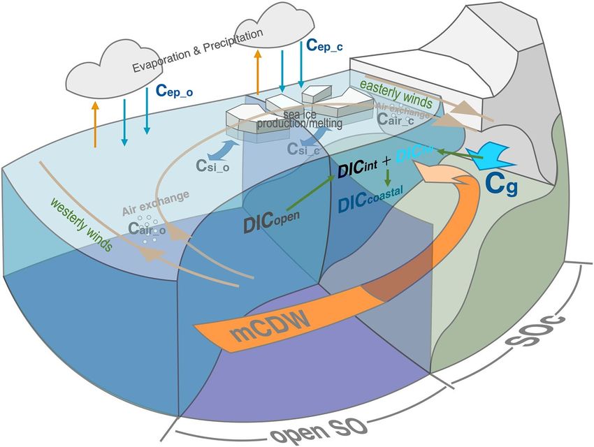
www.nature.com/scientificreports/
of method is in-situ observation. Long-term changes in seawater salinity can describe overall freshening which
includes all freshwater s ources12,19–21. Setting end-members (e.g. δ18O and salinity) to characterise each water
component is a common way to distinguish different sources of freshwater input6,18. However, it is difficult to
apply this method on a wide-scale because the end-members of water always change spatiotemporally.
To overcome these limitations and obtain a more comprehensive understanding of Antarctic glacier melting
and SOc freshening, parameterization technique has come into our view r ecently22–25. On the one hand, high-
accuracy observations of basic hydrographic parameters such as seawater temperature (T), salinity (S), dissolved
oxygen (DO), and pressure (Pr) have been conducted for nearly 100 years over the SO with a relatively higher
spatiotemporal resolution. Hence, the parameterization constructed by these basic hydrographic parameters
enables us to obtain more available data on various chemicals in the SO24. On the other hand, if T, S, DO, and
Pr are used in the parameterization function, a relationship reflecting the physical (e.g. water mass transporta-
tion) and biological (e.g. remineralization) processes can be obtained that relate to the chemical concentration
in a specific region. This functional relationship does not change unless it is influenced by any external process.
This suggests that for a parameterization of chemical A, the predicted concentration of A (Apre) contains a com-
ponent of the ocean internal processes ( Ain) and a component of the average external process ( Aex) within the
spatiotemporal range of the observed dataset used (Eq. 1). Based on the above two properties, parameterization
is often applied to the estimation of external material input in the ocean24,25.
Apre (T, S, DO . . .) = Ain (T, S, DO) + Aex . (1)
In this study, we propose a new method based on the interactions between Antarctic glacier and seawater and
the oceanic parameterization technique (hereafter referred to as “parameterization method”) that allows us to
estimate the glacier-derived freshening without setting any end-member so long as basic ocean hydrographic data
(T, S, DO, and Pr) are available. Applying this method to the Southern Ocean coastal oceans (SOc, seas around
Antarctica, here defined as the region where the seafloor is shallower than 1500 m, south of 60° S) using ocean
hydrographic data set from 1926 to 2016 were collected from the Global Ocean Data Analysis Project version 2
(GLODAPv2) and Southern Ocean Atlas (SOA)26,27, we obtained spatial distributions and multi-decadal time
series of the glacier-derived freshening over the SOc.
Results
Freshwater derived from glacier melting. Processes such as glacier melting, sea ice melting, and pre-
cipitation release large amounts of freshwater into the SO (Fig. 1). We treated these freshwater input as external
process which can change the dissolved inorganic carbon (DIC, used as the indicator of freshening here, see
“Methods” for details) concentration in seawater and assumed that this glacier melting is the only significant dif-
ferent external factor between the open ocean of the SO (open SO) and the SOc (see Eqs. 7–21 in the “Methods”
section). Then, we constructed the parameterizations of DIC for open SO and SOc, respectively. Both param-
eterizations can reconstruct DIC using T, S, apparent oxygen utilisation (AOU), and Pr from 0 m to the bottom
depth (Eqs. 2 and 3; see Supplementary Fig. S3 and “Methods” for details).
DICopen = a1 + a2 · AOUo + a3 · To + a4 · So + a5 · Pro
(2)
= 1024 + 0.5857 · AOUo − 8.452 · To + 33.38 · So + 1.798 × 10⁻³ · Pro
(Number of data points (n) = 46,753; coefficient of determination ( R2) = 0.98.
Root-mean-square error (RMSE) = 6.08 µmol kg−1)
DICcoastal = b1 + b2 · AOUc + b3 · Tc + b4 · Sc + b5 · Prc
(3)
= 43.75 + 0.3833 · AOUc − 4.817 · Tc + 62.43 · Sc
(n = 2059; R2 = 0.95; RMSE = 4.84 µmol kg−1),
where DICopen indicates the predicted DIC in the open SO; DICcoastal indicates the predicted DIC in the SOc;
a and b indicate the regression coefficients for these two parameterizations; subscript ‘o’ indicates parameter of
the open SO; subscript ‘c’ represents parameter of the SOc.
Based on the difference in DIC between these two parameterizations, we expressed the fraction of glacier-
derived freshwater in the SOc ( Fg), as shown in Eq. (4) (see “Methods” for details).
Fg = (DICint − DICcoastal )/DICint
= [(a1 − b1 ) + (a2 − b2 ) · AOUc + (a3 − b3 ) · Tc + (a4 − b4 ) · Sc (4)
+ (a5 − b5 ) · Prc ]/(a1 + a2 · AOUc + a3 · Tc + a4 · Sc + a5 · Prc ),
where DICint indicates the initial DIC concentration in the SOc without any freshwater input from the Antarctic
glacier (Eq. 15). A positive Fg indicates freshwater released from the Antarctic glacier to the SOc, leading to
freshening. The propagation of error derived from the DIC parameterizations suggests uncertainty in F g of ~ 36%.
Multi‑decadal time‑series of seawater freshening over the entire SOc. We applied our above-
mentioned parameterization method, to the observational hydrographic data in the SOc during 1926–2016,
which were collected from GLODAPv2 and SOA (23,449 data, almost in summertime)26,27, to estimate the time
series of freshening (shown as Fg) over SOc. To obtain the decadal change in freshening, we divided the data-
set into seven periods with approximately 10-year intervals (P1,1926–1955; P2,1956–1965; P3,1966–1975; P4,
1976–1985; P5,1986–1997; P6,1998–2006; P7,2007–2016). Regarding spatial division, we divided the SOc into
Scientific Reports | (2022) 12:383 | https://doi.org/10.1038/s41598-021-04231-6 2
Vol:.(1234567890)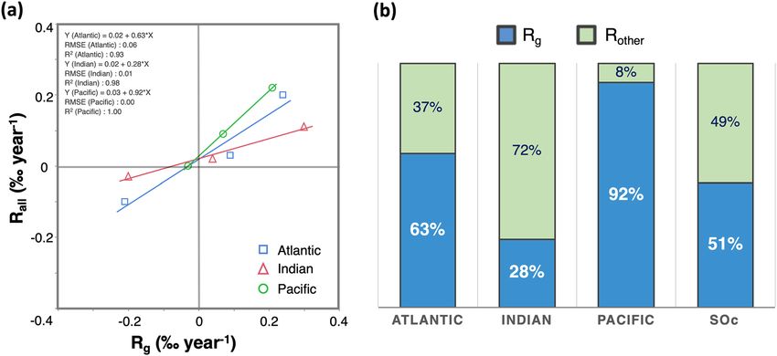
www.nature.com/scientificreports/
Figure 1. Interactions among the open SO, SOc, and Antarctic glacier. Without any freshwater input from
the Antarctic glacier, the initial seawater in the SOc entirely comes from the open SO with a DIC content of
DICint. Warm modified CDW (mCDW) inflows from the open SO into the ice cavity southwardly, leading to
ice shelf basal melt and freshwater release (with DIC = DICfw; shown by light blue arrows). The buoyant plume
of freshwater together with mCDW rises to the surface. The mixture of freshwater and initial seawater makes
the DIC concentration in the SOc become DICcoastal. ‘C’ indicates the DIC components which is controlled by
various external processes; subscripts ‘o’ and ‘c’ indicates processes of the open SO and the SOc, respectively;
subscripts ‘ep’, ‘si’, ‘air’ and ‘g’ indicates evaporation and precipitation, sea ice, air-sea exchange, and glacier
melting, respectively.
the Atlantic, Indian, and Pacific sectors which are mainly controlled by the ice shelves of the Antarctic Peninsula,
East Antarctica, and West Antarctica, respectively (Fig. 2b).
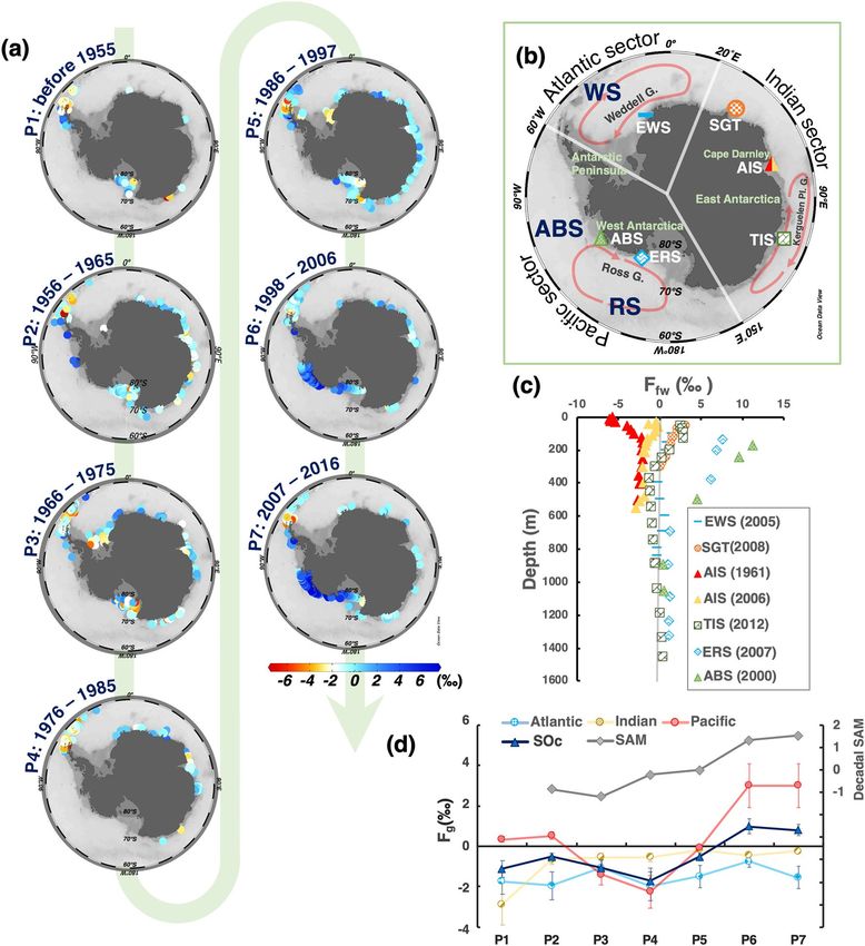
In both the Atlantic and Indian sectors, the averaged Fg values were generally near 0 during all periods
(Fig. 2a). However, in the Shirase Glacier Tongue (SGT, ~ 38° E) and Totten Ice Shelf (TIS, ~ 116° E), high basal
melt rates from the 2000s have been r eported5,6. Our estimate does show a positive F g in these regions (Fig. 2c).
Contrarily, in the Pacific sector, dramatic ice sheet mass loss and high basal melting have been reported to occur
in most regions over the last few decades, particularly over the Amundsen and Bellingshausen Seas (ABS, ~ 90°
W–150° W)7,28,29. Our estimate shows significant positive Fg over the Pacific sector, including ABS and Ross Sea,
during the late twentieth century to the early twenty-first century (Fig. 2a), which spatiotemporally agrees with
the above ice losses. Table 1 shows the rates of glacier-derived freshening ( Rg, Eq. 23) in the three sectors during
the seven periods. During P5 to P6, Rg in the Pacific sector reached 0.28 ± 0.14‰ year−1, while that in the whole
SOc was 0.14 ± 0.07‰ year−1.
Figure 2c shows the vertical profiles of F g in several focused regions, which have been reported to have
significant ice sheet mass loss. In the Pacific sector, the highest F g was 11 ± 4.0‰ in both ABS and the Eastern
Ross Sea (ERS) in the 2000s. In both the Indian and Atlantic sectors, we also found Fg reached 4.0 ± 1.5‰ at
the surface in the TIS, the SGT, and the Eastern Weddell Sea (EWS). At the Cape Darnley of the Indian sector,
which is an important region for sea ice and bottom water formations in East A ntarctica30, the mass balance of
the Amery Ice Shelf (AIS) has recently attracted extensive concern (Fig. 2b)12,31,32. In both 1961 and 2006, Fg
was almost negative [see AIS (1961) and AIS (2006) in Fig. 2c], implying that freshwater exchange is dominated
by freshwater consumption due to ice shelf freezing. Comparing the Fg in the AIS in 1961 with that in 2006, we
identified a positive trend in Fg (− 6 ± 2.2‰ to − 1 ± 0.4‰) from 1961 to 2006 (Fig. 2c), implying that ice shelf
freezing has been weakened, which may be related to mCDW intrusion31,32.
To quantify the impact of glacier-derived freshwater on the overall freshening in the SOc, we calculated the
rate of overall freshening ( Rall) in the SOc using the salinity trend divided by the average salinity of the research
region (Eq. 22). The correlations between R g and Rall in the three sectors of the SOc are shown in Fig. 3a. From
the slopes of the correlation lines, we found that during 1960–2016, glacier melting accounted for ~ 63%, ~ 28%,
and ~ 92% of the total freshening occurred in the Atlantic, Indian, and Pacific sectors of the SOc, respectively
(Fig. 3b). This suggests that glacier melting in West Antarctica and the Antarctic Peninsula plays a dominant
role in the freshening of the surrounding seas.
Scientific Reports | (2022) 12:383 | https://doi.org/10.1038/s41598-021-04231-6 3
Vol.:(0123456789)www.nature.com/scientificreports/
Region Area (km2) P1–P2a P2–P3 P3–P4 P4–P5 P5–P6 P6–P7
5
Atlantic 9.8 × 10 − 0.01 ± 0.01c 0.09 ± 0.04 − 0.09 ± 0.05 0.05 ± 0.02 0.07 ± 0.03 − 0.08 ± 0.04
Indian 8.6 × 10⁵ 0.11 ± 0.06 0.01 ± 0.01 0±0 0.04 ± 0.02 − 0.02 ± 0.01 0.02 ± 0.01
Pacific 1.4 × 10⁶ 0.01 ± 0 − 0.19 ± 0.1 − 0.09 ± 0.04 0.22 ± 0.11 0.28 ± 0.14 0±0
SOcb 3.3 × 10⁶ 0.03 ± 0.01 − 0.05 ± 0.03 − 0.06 ± 0.03 0.12 ± 0.06 0.14 ± 0.07 − 0.02 ± 0.01
Table 1. Rates of glacier-derived freshening (‰ year-−1) between each period during 1926 to 2016. a P1:
1926–1955, P2: 1956–1965, P3: 1966–1975, P4: 1976–1985, P5: 1986–1997, P6: 1998–2006, P7: 2007–2016.
b
Rates over the SOc are shown as the area weight average of the three sectors. c Error shows the uncertainty of
50% derived from the RMSE of the parameterizations and the propagation of errors arising in the subsequent
calculations.
We obtained the rate of glacier-derived freshwater input into the SOc by multiplying the regional average
g by the seawater volume. We found that the rate of glacier-derived freshwater input in the SOc reached a
R
maximum of 268 ± 134 Gt year−1 (74 ± 37 Gt y ear−1 as the lower limit, Supplementary Text S2) during the late
twentieth to early twenty-first centuries (1 Gt = 109 t = 1012 kg). If we assume that the melting of ice floe has no
significant variation on a decadal time-scale, we can consider that the difference between R g and R
all (Rother in
Fig. 3b) represents the rate of freshwater added by precipitation and melting of newly formed icebergs derived
from calving, which have the potential to raise the global sea-level by up to 0.7 ± 0.4 mm year−1.
Discussion
The mass balance of the Antarctic ice sheet is controlled by a combination of several p rocesses33. In the Pacific
sector, particularly in the ABS, much stronger freshening was observed than in the other two sectors. There is
evidence that teleconnections with tropics such as SAM and El Niño–Southern Oscillation (ENSO) contribute
significantly to the warm mCDW intrusion and the ice sheet mass loss in the A BS34. ABS is located near the
eastern limb of the Ross Gyre and is adjacent to the main stem of the Antarctic Circumpolar Current (ACC). This
geographic location is very conducive to the intrusion of mCDW into Antarctic ice cavities28. The Amundsen
Sea Low (low-pressure centre located over the southern Pacific) can also drive the transportation of warm air to
West Antarctica, which causes melting of the surface ice sheet and thereby contributes to freshening35.
For the Indian and Atlantic sectors, the basal melt rates are generally low because of the typical cold shelf in
this region36. However, our estimate and several previous studies showed that there were freshening signals in
specific regions such as TIS, AIS, and SGT (Fig. 2c)5,6,31,37. Except for the effect of the positive SAM, the loca-
tion and topographical conditions of these areas also play an unneglectable role. For instance, the SGT, which is
located at the eastern limb of the Weddell Gyre (Fig. 2b), the deep trough along the continental slope deep into
the ice front allows the mCDW to readily touch the ice s helf6.
We identified a significant positive correlation between Fg over SOc and the SAM index since 195538 (R = 0.82;
Fig. 2d and Supplementary Fig. S8), suggesting that a positive SAM is a possible contributor to the Antarctic ice
sheet mass loss. Forced by anthropogenic greenhouse gas emissions and stratospheric ozone depletion, SAM has
exhibited a positive trend since 1955, resulting in the intensification and southward shift of westerly winds10,38–40.
With the development of autonomous ocean observation robotics (Biogeochemical-Argo-float), we can obtain
more spatiotemporally complete basic hydrographic data in the SO. Applying our parameterization method to
the Bio-Argo-float d ataset41,42, it will be possible to perform quasi-real-time monitoring of interactions between
SOc and Antarctic glaciers and their impacts on the global ocean, which can greatly help us in a deeper under-
standing of global climate change in the future.
Methods
Data used in this study. The observational data used for constructing the parameterizations of DIC (DIC,
T, S, DO, and Pr) were sourced from GLODAPv2_2019 of the SO (south of 30° S) from 2000 to 201727. The qual-
ity of data on chemicals such as carbon species and nutrients after 2000 was controlled using certified reference
materials43. Therefore, high-accuracy data for these chemicals began to be obtained mainly after 2000. Basic
hydrographic data (T, S, DO, Pr) used to estimate the time series of freshening over the SOc were sourced from
GLODAPv2_2019 from 1979 to 2016 and SOA from 1926 to 1984 (south of 60° S, bottom depth shallower than
1500 m)26,27. Information on the cruises from which we obtained the data is shown in Supplementary Tables S1,
S2, and S3. Quality flags of the World Ocean Circulation Experiment (WOCE) were used to check the quality of
the data. In this study, we only used data with a quality flag of two (i.e. the data value is acceptable). To construct
the DIC parameterizations, we used 46,753 data points for D ICopen and 2059 data points for D ICcoastal from 2000
to 2017 (Supplementary Fig. S1). To estimate the time series of freshening, we used 23,449 data points from 1926
to 2016 (Supplementary Fig. S2).
Construction of DIC parameterizations and its quality validation. We used least-squares multiple
linear regression to construct the parameterizations of DIC in the SO, and we established for the first time DIC
parameterizations that can be applied to the entire SO from the surface ocean to the seafloor using T, S, AOU,
and Pr. AOU was calculated from DO and saturated oxygen concentration44. Several constraints were set for the
raw data (Supplementary Table S4).
Scientific Reports | (2022) 12:383 | https://doi.org/10.1038/s41598-021-04231-6 4
Vol:.(1234567890)www.nature.com/scientificreports/
Figure 2. Distributions of glacier-derived freshening over the SOc during 1926–2016. Freshening is represented
by the fraction of melt freshwater ( Fg, ‰). Positive values indicate freshwater released from the glacier into
the SOc, strengthening the freshening. (a) Spatiotemporal distributions of freshening over the SOc. Values
are shown as the average F g in the vertical water column. (b) Map of the Antarctic and the SO south of 60° S.
White lines separate the three sectors of the SOc (Atlantic Sector: 60° W–20° E; Indian Sector: 20° E–150° E;
Pacific Sector: 150° E–60° W). Blue abbreviations indicate the following seas: WS Weddell Sea, RS Ross Sea,
ABS Amundsen, and Bellingshausen Sea. White abbreviations indicate the stations in Fig. 2c; EWS Eastern
Weddell Sea, SGT Shirase Glacier Tongue, AIS Amery Ice Shelf, TIS Totten Ice Shelf, ERS Eastern Ross Sea, ABS
Amundsen, and Bellingshausen Seas. (c) Vertical distribution of Fg in several stations shown in Fig. 2b (white
abbreviations with symbols). (d) Decadal changes of Fg in the three sectors and the entire SOc during 1926–
2016 (left axis). Error bars show the uncertainty of 36% derived from the propagation of error. The grey line
indicates the decadal change of the Southern Annular Mode (SAM, right axis)38. Maps in this figure were drawn
using Ocean Data View 5.3.0 (https://odv.awi.de)47.
The F-test was used to examine the significance of each parameter in our parameterizations (Supplementary
Table S5). A parameter with an F-value greater than 2.4, was considered to have a significant effect. After a
stepwise regression, we selected AOU, T, S, and Pr for the DICopen; the F-values of each were 375,574, 464,617,
29,712, and 5505, respectively. Conversely, we used AOU, T, and S for the D ICcoastal, and the F-values of each
were 4,964,722, and 4080, respectively. The variance inflation factor (VIF) was used to investigate the presence
of multicollinearity between each parameter. Standardised regression coefficients (β) were used to compare
Scientific Reports | (2022) 12:383 | https://doi.org/10.1038/s41598-021-04231-6 5
Vol.:(0123456789)www.nature.com/scientificreports/
Figure 3. Impact of glacier melting on the SOc. (a) Correlations between the rate of glacier-derived freshening
( Rg) and overall freshening (Rall) in the SOc during 1960 ~ 2016. Blue open squares, red open triangles, and
green open circles indicate data picked up from Atlantic, Indian and Pacific sectors of SOc, respectively. Solid
lines are the correlation lines of each sector. Data used to plot this figure are given in Supplementary Table S8.
(b) Proportion of the rate of glacier-derived freshening ( Rg, shown in blue) and freshening derived from other
external processes (i.e. evaporation and precipitation and sea ice) ( Rother, shown in green) in each sector and the
entire SOc.
the contribution of each parameter to DIC (Supplementary Table S5). The closer the absolute value is to 1, the
greater the contribution of the parameter. AOU was the most significant parameter in both the open SO and
SOc. However, for the significance of T and S, D ICopen and D ICcoastal show the opposite pattern. The D ICopen is
mainly controlled by T, while the key parameter becomes S for the D ICcoastal, partly proving that DIC in the SOc
might have been affected by the input of melting freshwater.
We tested the accuracy of our parameterizations by conducting self-validation and cross-validation. First, we
used the dataset that was used in the construction of our parameterizations to perform self-validation. Supple-
mentary Figures S6 and S7 show the spatial distributions of the difference between the observed and predicted
DIC in the open SO and SOc, respectively. Most circumpolar regions (south of 50° S) showed no significant
difference, implying that there are no “blind spots” where our parameterization cannot be applied.
We conducted cross-validation using an independent testing dataset to further verify the reliability of our
parameterizations. For DIC parameterization in the open SO (DICopen), we selected one independent cruise for
each of the three sectors (Atlantic, Indian, and Pacific) that were not used in the construction of parameteriza-
tion as the testing data set (Supplementary Fig. S4). To quantify the extent of differences in DIC between the
independent observed data and D ICopen, we used the mean absolute deviations (MADs) as follows:
n
1
MADopen = DICobs_i − DICopen_i
, (5)
n
i=1
where MADopen indicates the MAD of DICopen, and n is the data amount of each independent testing dataset.
MADopen in the Pacific, Indian, and Atlantic sectors were 3.24, 2.48, and 5.06 µmol kg−1, respectively (Sup-
plementary Table S6). These MAD values are smaller than the RMSE of DICopen (6.08 µmol kg−1), implying
that DICopen has sufficient reliability. In contrast, for the parameterization of SOc ( DICcoastal), the sparseness of
observational data makes it difficult to find additional independent testing datasets for accuracy validation. To
check the reliability of DICcoastal, we used the “k-fold cross-validation”45,46. The k-fold cross-validation uses part
of the available data to construct the parameterization (training dataset) and uses the remaining part to test it
(testing dataset). Here, we divided the observational data set into 10 roughly equal-sized groups by longitude
(i.e. k = 10), using one group as the testing dataset and the remaining nine groups as the training data set. We
then exchanged other groups as the testing dataset and the remaining nine groups as the training dataset. We
repeated the above process nine times. The MAD of DICcoastal (MADcoastal) is similar to that in Eq. (5):
n
1
MADcoastal = DICobs_i − DICcoastal_i
. (6)
n
i=1
The results of the k-fold cross-validation for the SOc are shown in Supplementary Fig. S5 and Supplementary
Table S7.
Scientific Reports | (2022) 12:383 | https://doi.org/10.1038/s41598-021-04231-6 6
Vol:.(1234567890)www.nature.com/scientificreports/
In the surface layer of both the open SO and the SOc, the differences in DIC between the validation observed
data and our parameterizations are relatively large, which is probably due to the air-sea exchange and the seasonal
differences between the observational data used.
Quantification of glacier‑derived freshwater input in the SOc. As discussed in the main text, for
the parameterization of chemical A, the predicted value of A (Apre) contains a term for the ocean internal pro-
cesses (Ain) and a term of the average external process (Aex) within the spatiotemporal range of the observed
dataset used (Eq. 1). Therefore, when we construct parameterizations for DIC in the open SO and SOc, they also
satisfy this property (Eqs. 7–9 and 10–12).
DICopen = DICin_o + DICex_o , (7)
DICin_o = Cbio_o + Cphy_o , (8)
DICex_o = Cep_o + Csi_o + Cair_o , (9)
DICcoastal = DICin_c + DICex_c , (10)
DICin_c = Cbio_c + Cphy_c , (11)
DICex_c = Cep_c + Csi_c + Cair_c + Cg , (12)
where DICopen is defined as the predicted DIC in the open SO; DICcoastal is defined as the predicted DIC in the
SOc; subscripts ‘in’ and ‘ex’ indicates terms of DIC concentrations which are controlled by internal processes and
external processes of the ocean, respectively; subscripts ‘o and ‘c’ indicates terms of the open SO and the SOc,
respectively. DICin mainly includes two components: the biological components ( Cbio) and the physical compo-
nents (Cphy), which can be represented by the parameters (T, S, AOU, Pr). The D ICex includes the evaporation
and precipitation components (Cep), sea ice (i.e. floating ice, iceberg) components (Csi), and air-sea exchange
components (Cair) in both the open SO and the SOc. It is worth noting that in the SOc, there is a unique external
DIC component derived from the Antarctic glacier (Cg).
We quantified the fraction of glacier-derived freshwater in the SOc (Fg) based on the above parameteriza-
tions and processes shown in Fig. 1. The seawater in the SOc consists of two components: one is the seawater
coming from the open SO (referred to as initial seawater, with DIC concentration of DICint), and the other is
the external freshwater added into the SOc (with DIC concentration of DICfw). The relationship between these
water components can be expressed by the following conservation equations:
Ffw + Fopen = 1, (13)
Ffw · DICfw + Fint · DICint = Ffw · 0 + Fint · DICint
(14)
= DICcoastal ,
where Fint is the fraction of the initial seawater. Ffw is the fraction of freshwater added to SOc. DICfw was assumed
to be equal to zero.
Assuming that the initial seawater in the SOc comes entirely from the open SO, this allows us to calculate
DICint by substituting the parameters of the SOc into the open ocean parameterization ( DICopen).
DICint = DICopen (Tc , Sc , AOUc , Prc ) = DICin_c + DICex_o . (15)
ICin is completely controlled by the parameters (T, S, AOU, Pr), so when we substitute the
Note that here D
parameters of the SOc into D ICopen, DICin becomes D
ICin_c, whereas D
ICex remains as D
ICex_o because this term
is binding to D
ICopen. Combining Eq. (13) with Eq. (14), we obtain Ffw as follows.
Ffw = (DICint − DICcoastal ) / DICint . (16)
Then substituting Eqs. (7–9) and (10–12) into Eq. (16), we obtain the following equation:
Ffw = DICin_c + DICex_o − DICin_c + DICex_c / DICint .
(17)
= DICin_c − DICin_c + DICex_o − DICex_c / DICint .
= Cep_o − Cep_c + Csi_o − Csi_c + Cair_o − Cair_c − Cg / DICint .
ep, Csi, and Cair exist in both the open SO and SOc. Therefore, we assume that
The external components C
Cep_o ≈ Cep_c , (18)
Csi_o ≈ Csi_c , (19)
Cair_o ≈ Cair_c . (20)
Scientific Reports | (2022) 12:383 | https://doi.org/10.1038/s41598-021-04231-6 7
Vol.:(0123456789)www.nature.com/scientificreports/
Finally, by substituting Eqs. (18–20) into Eq. (17), we obtain Ffw as Eq. (21):
(21)
Ffw = −Cg / DICint = Fg .
We found that F fw is only controlled by the glacier-derived term, implying that the freshwater estimated by
this method can be considered as the freshwater derived from Antarctic glacier melting ( Fg).
We attempted to use various oceanic chemicals, including DIC, nitrate, and phosphate, as indicators of
freshwater input. The essential advantage of DIC compared with other chemicals is that it maintains a relatively
good linear relationship with hydrographic parameters, even within the surface mixed layer. Especially in the
open ocean, the concentration of nutrients in the surface mixed layer is almost zero, which makes it difficult to
construct parameterizations. Therefore, DIC was chosen as the freshwater indicator.
The average Fg in each sector of the SOc shown in Fig. 2d were calculated after gridding the raw data shown in
Fig. 2a. This is done to lower the impact of spatial bias in the raw data distribution. We interpolated the raw data
onto a 1° × 1° grid with a scale-length of 5° of longitude and 1° of latitude using the Ocean Data View software
(Supplementary Fig. S10)47. The area of each grid was also considered when calculating the average, since the area
of the grid varies with latitude. The average Fg of the SOc is shown as the area weight average of the three sectors.
We changed the fraction of freshwater into volume by multiplying the fraction by the seawater volume. The
seawater volumes used here were calculated by multiplying the average depth of all data profiles by the ocean
surface area of the SOc or the three sectors. The ocean surface areas are listed in Table 1.
Calculation of the rate of overall freshening in the SOc based on the salinity trend. To quantify
the impact of glacier melting on the SOc, we calculated the rate of overall freshening in the SOc according to
the following steps: It is impossible to estimate the fraction of freshwater at a given moment through the salinity.
Thus, we simply estimated the rate of freshening based on the rate of salinity change.
Rall = (dSobs /dt) / Save , (22)
where R all indicates the rate of overall freshening in the SOc; dSobs/dt indicates the observed salinity trend,
which is controlled by evaporation and precipitation, sea ice, and glaciers, and Save is the average salinity over
our research region (Save = 34.3).
The rate of glacier-derived freshening ( Rg) is calculated as follow:
Rg = dFg /dt. (23)
Data availability
Hydrographic data and DIC data after 2000 used to construct DIC parameterizations are available in GLODAP
v2 2020 (https://www.glodap.info/index.php/data-access/). Hydrographic data from 1926 to 2016 used to esti-
mate freshwater input are available in GLODAP v2 2020 and Southern Ocean Atlas (https://odv.awi.de/data/
ocean/southern-ocean-atlas/). See a detailed description of the data used in this study in the Methods section.
Received: 16 June 2021; Accepted: 15 December 2021
References
1. Vaughan, D. G. et al. In Climate Change 2013: The Physical Science Basis. Contribution of Working Group I to the Fifth Assessment
Report of the Intergovernmental Panel on Climate Change (eds Stocker, T. F. et al.) Ch. 4, 317–382 (Cambridge University Press,
2013).
2. Rignot, E. et al. Four decades of Antarctic Ice Sheet mass balance from 1979–2017. Proc. Natl. Acad. Sci. U.S.A. 116, 1095–1103.
https://doi.org/10.1073/pnas.1812883116 (2019).
3. Church, J. A. et al. In Climate Change 2013: The Physical Science Basis. Contribution of Working Group I to the Fifth Assessment
Report of the Intergovernmental Panel on Climate Change (eds Stocker, T. F. et al.) Ch. 13, 1137–1216 (Cambridge University Press,
2013).
4. Rye, C. D. et al. Rapid sea-level rise along the Antarctic margins in response to increased glacial discharge. Nat. Geosci. 7, 732–735.
https://doi.org/10.1038/ngeo2230 (2014).
5. Rintoul, S. R. et al. Ocean heat drives rapid basal melt of the Totten Ice Shelf. Sci. Adv. 2, e1601610. https://doi.org/10.1126/sciadv.
1601610 (2016).
6. Hirano, D. et al. Strong ice-ocean interaction beneath Shirase Glacier Tongue in East Antarctica. Nat. Commun 11, 4221. https://
doi.org/10.1038/s41467-020-17527-4 (2020).
7. Rignot, E., Jacobs, S., Mouginot, J. & Scheuchl, B. Ice-shelf melting around Antarctica. Science 341, 266–270. https://doi.org/10.
1126/science.1235798 (2013).
8. Mizobata, K., Shimada, K., Aoki, S. & Kitade, Y. The cyclonic eddy train in the Indian Ocean sector of the southern ocean as revealed
by satellite radar altimeters and in situ measurements. J. Geophys. Res. Oceans. https://doi.org/10.1029/2019jc015994 (2020).
9. Dinniman, M. et al. Modeling ice shelf/ocean interaction in Antarctica: A review. Oceanography 29, 144–153. https://doi.org/10.
5670/oceanog.2016.106 (2016).
10. Saenko, O. A., Fyfe, J. C., Zickfeld, K., Eby, M. & Weaver, A. J. The role of poleward-intensifying winds on southern ocean warming.
J. Clim. 20, 5391–5400. https://doi.org/10.1175/2007jcli1764.1 (2007).
11. Liu, Y. et al. Ocean-driven thinning enhances iceberg calving and retreat of Antarctic ice shelves. Proc. Natl. Acad. Sci. U.S.A. 112,
3263–3268. https://doi.org/10.1073/pnas.1415137112 (2015).
12. Aoki, S. et al. Freshening of Antarctic bottom water off Cape Darnley, East Antarctica. J. Geophys. Res. Oceans. https://doi.org/10.
1029/2020jc016374 (2020).
13. Aoki, S., Rintoul, S. R., Ushio, S., Watanabe, S. & Bindoff, N. L. Freshening of the Adélie Land Bottom Water near 140°E. Geophys.
Res. Lett. https://doi.org/10.1029/2005gl024246 (2005).
Scientific Reports | (2022) 12:383 | https://doi.org/10.1038/s41598-021-04231-6 8
Vol:.(1234567890)www.nature.com/scientificreports/
14. Johnson, G. C., Purkey, S. G. & Bullister, J. L. Warming and freshening in the Abyssal Southeastern Indian Ocean. J. Clim. 21,
5351–5363. https://doi.org/10.1175/2008jcli2384.1 (2008).
15. Purkey, S. G. & Johnson, G. C. Antarctic bottom water warming and freshening: contributions to sea level rise, ocean freshwater
budgets, and global heat gain. J. Clim. 26, 6105–6122. https://doi.org/10.1175/jcli-d-12-00834.1 (2013).
16. Rhein, M. et al. In Climate Change 2013: The Physical Science Basis. Contribution of Working Group I to the Fifth Assessment Report
of the Intergovernmental Panel on Climate Change (eds Stocker, T. F. et al.) Ch. 3, 255–316 (Cambridge University Press, 2013).
17. Adusumilli, S., Fricker, H. A., Medley, B., Padman, L. & Siegfried, M. R. Interannual variations in meltwater input to the Southern
Ocean from Antarctic ice shelves. Nat. Geosci. 13, 616–620. https://doi.org/10.1038/s41561-020-0616-z (2020).
18. Silvano, A. et al. Freshening by glacial meltwater enhances melting of ice shelves and reduces formation of Antarctic Bottom Water.
Sci. Adv. 4, eaap9467. https://doi.org/10.1126/sciadv.aap9467 (2018).
19. Aoki, S. et al. Reversal of freshening trend of Antarctic Bottom Water in the Australian-Antarctic Basin during 2010s. Sci. Rep. 10,
14415. https://doi.org/10.1038/s41598-020-71290-6 (2020).
20. Hellmer, H. H., Huhn, O., Gomis, D. & Timmermann, R. On the freshening of the northwestern Weddell Sea continental shelf.
Ocean Sci. 7, 305–316. https://doi.org/10.5194/os-7-305-2011 (2011).
21. Jacobs, S. S., Giulivi, C. F. & Mele, P. A. Freshening of the Ross Sea during the late 20th century. Science 297, 386–389. https://doi.
org/10.1126/science.1069574 (2002).
22. Li, B., Watanabe, Y. W. & Yamaguchi, A. Spatiotemporal distribution of seawater pH in the North Pacific subpolar region by using
the parameterization technique. J. Geophys. Res. Oceans 121, 3435–3449. https://doi.org/10.1002/2015jc011615 (2016).
23. Li, B. F., Watanabe, Y. W., Hosoda, S., Sato, K. & Nakano, Y. Quasi-real-time and high-resolution spatiotemporal distribution of
ocean anthropogenic C O2. Geophys. Res. Lett. 46, 4836–4843. https://doi.org/10.1029/2018gl081639 (2019).
24. Pan, X. L., Li, B. F. & Watanabe, Y. W. The Southern Ocean with the largest uptake of anthropogenic nitrogen into the ocean interior.
Sci. Rep. 10, 8838. https://doi.org/10.1038/s41598-020-65661-2 (2020).
25. Clement, D. & Gruber, N. The eMLR(C*) method to determine decadal changes in the global ocean storage of anthropogenic CO2.
Glob. Biogeochem. Cycles 32, 654–679. https://doi.org/10.1002/2017gb005819 (2018).
26. Olbers, D. G., Viktor, V., Seiß, G. & Schröter, J. Hydrographic Atlas of the Southern Ocean in original file formats. PANGAEA
https://doi.org/10.1594/PANGAEA.750658 (2010).
27. Olsen, A. et al. GLODAPv2.2019—An update of GLODAPv2. Earth Syst. Sci. Data 11, 1437–1461. https://doi.org/10.5194/essd-
11-1437-2019 (2019).
28. Nakayama, Y., Menemenlis, D., Zhang, H., Schodlok, M. & Rignot, E. Origin of Circumpolar Deep Water intruding onto the
Amundsen and Bellingshausen Sea continental shelves. Nat. Commun. 9, 3403. https://d oi.o
rg/1 0.1 038/s 41467-0 18-0 5813-1 (2018).
29. Bingham, R. G. et al. Inland thinning of West Antarctic Ice Sheet steered along subglacial rifts. Nature 487, 468–471. https://doi.
org/10.1038/nature11292 (2012).
30. Ohshima, K. I. et al. Antarctic Bottom Water production by intense sea-ice formation in the Cape Darnley polynya. Nat. Geosci.
6, 235–240. https://doi.org/10.1038/ngeo1738 (2013).
31. Wen, J. et al. Basal melting and freezing under the Amery Ice Shelf, East Antarctica. J. Glaciol. 56, 81–90. https://doi.org/10.3189/
002214310791190820 (2017).
32. Williams, G. D. et al. The suppression of Antarctic bottom water formation by melting ice shelves in Prydz Bay. Nat. Commun. 7,
12577. https://doi.org/10.1038/ncomms12577 (2016).
33. Noble, T. L. et al. The sensitivity of the Antarctic Ice sheet to a changing climate: Past, present, and future. Rev. Geophys. https://
doi.org/10.1029/2019rg000663 (2020).
34. Steig, E. J., Ding, Q., Battisti, D. S. & Jenkins, A. Tropical forcing of Circumpolar Deep Water Inflow and outlet glacier thinning
in the Amundsen Sea Embayment, West Antarctica. Ann. Glaciol. 53, 19–28. https://doi.org/10.3189/2012AoG60A110 (2017).
35. Raphael, M. N. et al. The Amundsen sea low: Variability, change, and impact on Antarctic climate. Bull. Am. Meteorol. Soc 97,
111–121. https://doi.org/10.1175/bams-d-14-00018.1 (2016).
36. Schmidtko, S., Heywood, K. J., Thompson, A. F. & Aoki, S. Multidecadal warming of Antarctic waters. Science 346, 1227–1231.
https://doi.org/10.1126/science.1256117 (2014).
37. Nicholls, K. W. et al. A ground-based radar for measuring vertical strain rates and time-varying basal melt rates in ice sheets and
shelves. J. Glaciol. 61, 1079–1087. https://doi.org/10.3189/2015JoG15J073 (2017).
38. Marshall, G. J. Trends in the Southern Annular mode from observations and reanalyses. J. Clim. 16, 4134–4143. https://doi.org/
10.1175/1520-0442(2003)016%3c4134:Titsam%3e2.0.Co;2 (2003).
39. Stammerjohn, S. E., Martinson, D. G., Smith, R. C., Yuan, X. & Rind, D. Trends in Antarctic annual sea ice retreat and advance
and their relation to El Niño-Southern Oscillation and Southern Annular Mode variability. J. Geophys. Res. https://doi.org/10.
1029/2007jc004269 (2008).
40. Thompson, D. W. J. et al. Signatures of the Antarctic ozone hole in Southern Hemisphere surface climate change. Nat. Geosci. 4,
741–749. https://doi.org/10.1038/ngeo1296 (2011).
41. Fumihiko, A. et al. Argo float data and metadata from Global Data Assembly Centre (Argo GDAC). SEANOE https://doi.org/10.
17882/42182 (2020).
42. Talley, L. D. et al. Southern Ocean biogeochemical float deployment strategy, with example from the greenwich meridian line
(GO-SHIP A12). J. Geophys. Res. Oceans 124, 403–431. https://doi.org/10.1029/2018JC014059 (2019).
43. Dickson, A. G., Sabine, C. L. & Christian, J. R. Guide to best practices for ocean CO2 measurements. PICES Spec. Publ. 191 (2007).
44. Weiss, R. F. The solubility of nitrogen, oxygen and argon in water and seawater. Deep-Sea Res. Oceanogr. Abstr. 17, 721–735. https://
doi.org/10.1016/0011-7471(70)90037-9 (1970).
45. Hastie, T., Tibshirani, R. & Friedman, J. H. The Elements of Statistical Learning: Data Mining, Inference, and Prediction (Springer,
2009).
46. Fushiki, T. Estimation of prediction error by using K-fold cross-validation. Stat. Comput. 21, 137–146. https://doi.org/10.1007/
s11222-009-9153-8 (2009).
47. Schlitzer, R. Ocean Data View, https://odv.awi.de (2021).
Acknowledgements
We would like to thank the GLODAP group and all researchers who contributed to the construction of the global
ocean databases. We are grateful to Dr. Hirano of Hokkaido University for his insightful comments. This study
was partially supported by the Ministry of Education, Culture, Sports, Science, and Technology, Japan (Grant
number KAKEN 18H04131, 20H04962).
Author contributions
X.L.P. and Y.W.W. provided the central idea for this study, X.L.P. compiled the data sets, X.L.P. and B.F.L. analysed
the data, and X.L.P., B.F.L., and Y.W.W. co-wrote the paper.
Scientific Reports | (2022) 12:383 | https://doi.org/10.1038/s41598-021-04231-6 9
Vol.:(0123456789)www.nature.com/scientificreports/
Competing interests
The authors declare no competing interests.
Additional information
Supplementary Information The online version contains supplementary material available at https://doi.org/
10.1038/s41598-021-04231-6.
Correspondence and requests for materials should be addressed to X.L.P.
Reprints and permissions information is available at www.nature.com/reprints.
Publisher’s note Springer Nature remains neutral with regard to jurisdictional claims in published maps and
institutional affiliations.
Open Access This article is licensed under a Creative Commons Attribution 4.0 International
License, which permits use, sharing, adaptation, distribution and reproduction in any medium or
format, as long as you give appropriate credit to the original author(s) and the source, provide a link to the
Creative Commons licence, and indicate if changes were made. The images or other third party material in this
article are included in the article’s Creative Commons licence, unless indicated otherwise in a credit line to the
material. If material is not included in the article’s Creative Commons licence and your intended use is not
permitted by statutory regulation or exceeds the permitted use, you will need to obtain permission directly from
the copyright holder. To view a copy of this licence, visit http://creativecommons.org/licenses/by/4.0/.
© The Author(s) 2022
Scientific Reports | (2022) 12:383 | https://doi.org/10.1038/s41598-021-04231-6 10
Vol:.(1234567890)You can also read