In-stream Energy by Tidal and Wind-driven Currents: An Analysis for the Gulf of California
←
→
Page content transcription
If your browser does not render page correctly, please read the page content below
Preprints (www.preprints.org) | NOT PEER-REVIEWED | Posted: 24 February 2020                       doi:10.20944/preprints202002.0216.v2

                           Peer-reviewed version available at Energies 2020, 13, 1095; doi:10.3390/en13051095

              Article
              In-stream Energy by Tidal and Wind-driven Currents:
              An Analysis for the Gulf of California
              Vanesa Magar 1,†,∗ , Victor M. Godínez 1,† , Markus S. Gross1 , Manuel López-Mariscal1 ,
              Anahí Bermúdez-Romero1 , J. Candela1 and L. Zamudio 2
                1   Physical Oceanography Department, CICESE, Carretera Ensenada-Tijuana No. 3918, Zona Playitas,
                    Ensenada C.P. 22860, Baja California, Mexico
                2   Center for Ocean-Atmospheric Prediction Studies, Florida State University, Tallahassee, FL 32306-2840
               *    Correspondence: vmagar@cicese.edu.mx; Tel: +52-1646-175-0500
               †    These authors contributed equally to this work.

               Abstract: We analyzed the peak spring tidal current speeds, annual mean tidal power densities
               (TPD) and annual energy production (AEP) obtained from experiment 06.1, referred as the "HYCOM
               model" throughout, of the three dimensional (3D), global model HYCOM in an area covering the
               Baja California Pacific and the Gulf of California. The HYCOM model is forced with astronomical
               tides and surface winds alone, and therefore is particularly suitable to assess the tidal current and
               wind-driven current contribution to in-stream energy resources. We find two areas within the Gulf of
               California, one in the Great Island Region and one in the Upper Gulf of California, where peak spring
               tidal flows reach speeds of 1.1 meters per s econd. Second to fifth-generation tidal stream devices
               would be suitable for deployment in these two areas, which are very similar in terms of tidal in-stream
               energy resources. However, they are also very different in terms of sediment type and range in water
               depth, posing different challenges for in-stream technologies. The highest mean TPD value when
               excluding TPDs equal or less than 50 W m−2 (corresponding to the minimum velocity threshold for
               energy production) is of 172.8 W m−2 , and is found near the town of San Felipe, at (lat lon) = (31.006
               -114.64); here energy would be produced during 39.00% of the time. Finally, wind-driven currents
               contribute very little to the mean TPD and the total AEP. Therefore, the device, the grid, and any
               energy storage plans need to take into account the periodic tidal current fluctuations, for optimal
               exploitation of the resources.

                Keywords: Tidal Power Density; In-Stream Renewable Energy; Peak Spring Tide Flow; Annual
                Energy Production; Gulf of California

              1. Introduction
                   Tides, winds, and density gradients contribute to the generation, the characteristics, and the
              evolution of ocean currents, but their percentage contribution may vary in space and time. In the
              open ocean, tidal currents are assumed to play a small role because the water depth is usually large.
              In contrast, in estuaries, inlets, and marginal seas, the tidal amplitudes and speeds increase due to
              funnelling and resonance effects caused by the bathymetry and the geometry of the basin. Tidal
              currents can be identified very easily in in-situ measurements or numerical simulations, because the
              tidal forcing is harmonic with well defined frequencies given by the tidal potential [1,2]. However,
              in general it is more complex to separate the residual current into wind-driven and density-driven
              components, except when one develops or applies a numerical model that is only forced with tides
              and with surface wind fields. Two of such models have been found in the literature, one is the global
              HYCOM model reported in [3,4], and the other is the regional Delft3D model reported in [5]. In this

            © 2020 by the author(s). Distributed under a Creative Commons CC BY license.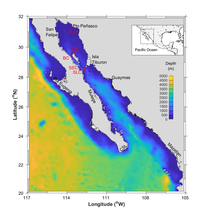
Preprints (www.preprints.org) | NOT PEER-REVIEWED | Posted: 24 February 2020                 doi:10.20944/preprints202002.0216.v2

                         Peer-reviewed version available at Energies 2020, 13, 1095; doi:10.3390/en13051095

                                                                                                                 2 of 18

              work we will use the global HYCOM model, because with a global model other authors can replicate
              more easily our analysis at other sites around the world.
                    From a renewable energy characterization perspective, there are multiple studies that have
              assessed water level ranges for tidal barrages or tidal lagoons [6–8], and tidal and marine current
              speeds for in-stream device deployments [9–12], at different sites. Tidal barrages and lagoons exploit
              potential energy, while in-stream devices exploit hydrokinetic energy. Most studies focus on either
              tidal lagoons or in-stream devices only, because generally the best energy exploitation sites for each of
              these types of marine renewable energy (MRE) do not overlap. Also, the energy conversion devices
              themselves, together with the necessary infrastructure, may be different. Here we focus on hydrokinetic
              energy generation, and specifically on tidal and wind-driven current energy resources.
                    From an economic perspective it makes more sense to consider one development at a time, and
              ensure best return on investment before moving on. However, in some specific cases, such as in the
              MERMAID project (see http://www.vliz.be/projects/mermaidproject/), assessing a combination of
              options for the development of Multi-Use Platforms at Sea (MUPS) is the main deliverable, and some
              case studies within MERMAID have considered co-location of wind and wave conversion devices [13],
              for example. Some companies are exploring whether combining these technologies is financially robust
              (see http://www.floatingpowerplant.com/), but most studies conclude that such combinations are
              financially sound for co-location of multiple users, such as marine renewable energy, aquaculture and
              platform related transport, rather than co-location of different renewable energy technologies [14,15].
                    The purpose of this paper is to characterize the tidal currents and wind-driven currents in the
              Gulf of California, with some comments about tidal resources in the Baja Californian Pacific, and
              analyze their respective contributions to in-stream renewable energy generation. This is relevant to
              the MRE Industry because it informs them on most appropriate development sites in the region, and
              they can adapt their technological developments based on the findings. It is also relevant from a
              scientific point of view, because there are very few studies focusing on this particular issue, either
              under climatologically normal or under extreme conditions. The paper is organized as follows. In
              Sec. 2, we present the model validations, and evaluate the contribution of the barotropic tidal currents
              and the wind-driven currents to the mean peak flow speeds, in-stream power density, and annual
              energy production. In Sec. 3, we describe the HYCOM model configuration used in this work. We
              also describe the in-situ measurements and the methodology adopted for the verification of the model
              predictions. In Sec. 4, we close with some concluding remarks.

              2. Results and Discussion
                   The HYCOM model is used to analyse the percentage contributions to Tidal Power Density (TPD)
              and Annual Energy Production (AEP), of the wind-driven currents and the tidally-driven currents.
              The analysis is performed over the domain and with the bathymetry shown in Fig. 1. The red markers
              in the Great Island Region (GIR) correspond to ADCP moorings in the San Lorenzo Channel (SLC),
              the San Esteban Channel (SEC), the Ballenas Channel (BC). and the Delfin Sill (DS). Another ADCP
              mooring near Isla San Jorge (ISJ) was also used for verification.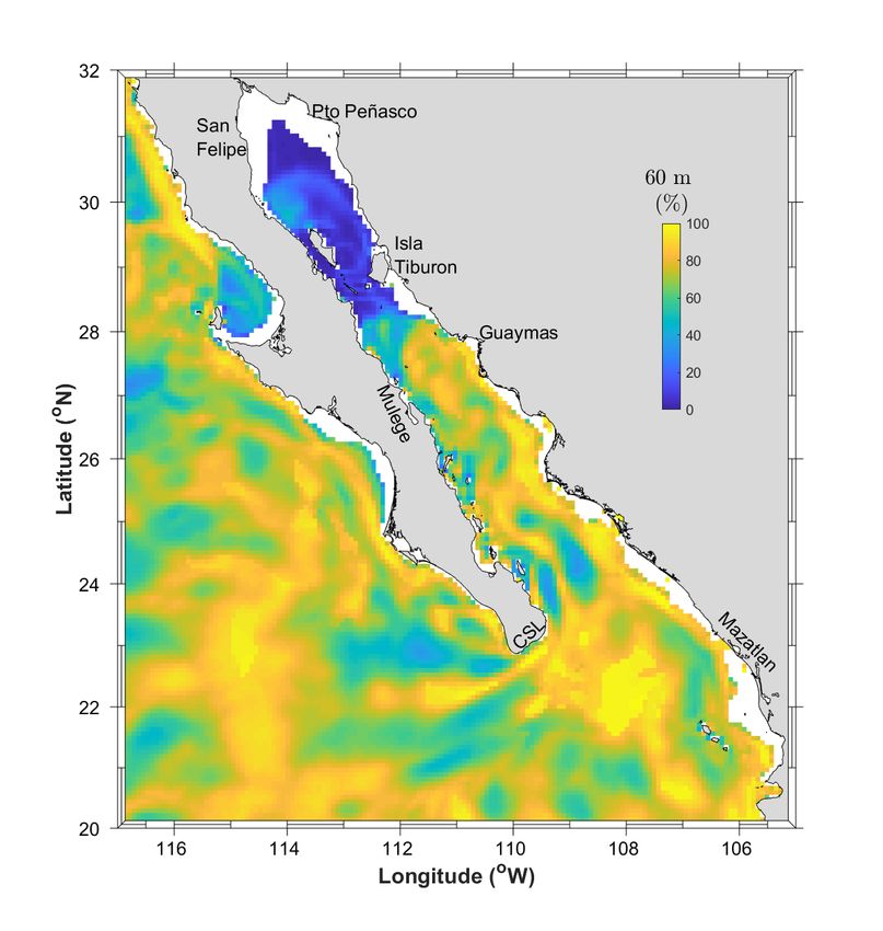
Preprints (www.preprints.org) | NOT PEER-REVIEWED | Posted: 24 February 2020                     doi:10.20944/preprints202002.0216.v2

                          Peer-reviewed version available at Energies 2020, 13, 1095; doi:10.3390/en13051095

                                                                                                                     3 of 18

                            Figure 1. Model domain and bathymetry with markers showing ADCP moorings.

              2.1. Verification of model predictions against in-situ measurements
                    Fig. 2 shows the vertically-integrated flow speed obtained with the HYCOM model (in red) and
              the measurements (in dashed blue) from the 1st of October to the 16th of October 2011, in the San
              Esteban Channel (SEC) mooring (shown in Fig. 1). The verification is carried out for the barotropic tidal
              currents only, and to compare the hourly tidal current time series obtained from the measurements to
              those from the model, the former had to be reconstructed for the period of simulation of the latter, i.e.
              for the period between 01/10/2011 01:00:00 and 01/10/2012 00:00:00 - this is explained in more detail
              in Sec. 3. Table 1 shows the yearly average of the modelled (mod) and measured (obs) values (shown
              next to each other in "mod/obs" format) of U (see Eqn. 1), TPD (see Eqn. 2), the AEP (see Eqn. 3), the
              relative error REx (see Eqn. 5) and the RMSEx (see Eqn. 6) for x = U and x = TPD, as well as the
              correlation coefficient ρ X,Y (see Eqn. 4), at the five verification sites. In the GIR ρ X,Y is either 0.91 or
              0.92, and it is 0.71 at ISJ. ρ X,Y is much lower at ISJ because the bathymetry used by the model in the
              region of San Jorge Bay is not as good as the bathymetry used in the GIR. Please note that no results of
              the RE or RMSE for AEP are shown because they are the same as for the TPD.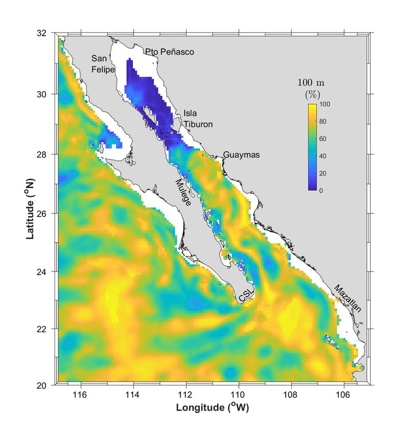
Preprints (www.preprints.org) | NOT PEER-REVIEWED | Posted: 24 February 2020                      doi:10.20944/preprints202002.0216.v2

                         Peer-reviewed version available at Energies 2020, 13, 1095; doi:10.3390/en13051095

                                                                                                                     4 of 18

                                              Table 1. Verification table for mean values.

                                           h     i     h       i                               h      i
                       Units: U m s−1 , TPD W m−2 , AEP kWh m−2 , RE [%], RMSEU m s−1 , RMSETPD W m−2


               Mooring    U mod/obs     TPD mod/obs       AEP mod/obs       ρ X,Y     REU     RETPD      RMSEU       RMSETPD
                 ISJ      0.202/0.206    7.56/10.48         66.45/92.07     0.71     2.0%     27.8%     9.1 × 10⁻²    14.13
                 DS       0.182/0.182     7.44/7.67         65.35/67.33     0.92     0.2%      3%       4.8 × 10⁻²     6.05
                 BC       0.190/0.360    8.69/60.60         76.33/532.3     0.92      47%      86%      21 × 10−2      98.2
                SEC       0.372/0.417    56.28/85.24       494.4 / 748.7    0.91     10.8%     34%     11.7 × 10⁻²    63.98
                SLC       0.263/0.388    21.98/72.75        193.1/639.1     0.92     32.2%    69.8%    17.3 × 10⁻²    102.0

                  The model underestimates U and TPD at all verification sites. The agreement is significantly
              worse at BC and at SLC, the two moorings furthest to the west. However, good agreement between
              model and observations is obtained at DS, ISJ and SEC. We also have significantly worse agreement at
              BC and at SLC for the annual mean maximum spring tide speeds and TPD, shown in Table 2, but the
              REU and RMSEU at the other three sites, are less than 10% and less than 3.7 × 10⁻¹ m s−1 , respectively.

                                   Table 2. Verification table for mean maximum spring tidal values.

                                                    h     i                       h      i
                                Units: U m s−1 , TPD W m−2 , RMSEU m s−1 , RMSETPD W m−2


                    Mooring    U STM mod/obs      TPD STM mod/obs        REU        RETPD      RMSEU       RMSETPD
                      ISJ        0.415/0.459        38.76/55.80          9.8%       30.6 %   11.9 × 10⁻²    38.56
                      DS         0.417/0.399         39.6/35.62         -4.6%       -11.2%   4.5 × 10⁻²     12.23
                      BC         0.467/0.822         54.6/311.1         43.2%        82.5%   36.7 × 10⁻²    290.2
                     SEC         0.866/0.928        347.4 /437.7         6.6%        20.6%   8.3 × 10⁻²     119.36
                     SLC         0.568/0.918        101.7/436.7         38.2%        76.7%   36.8 × 10⁻²    390.6

                   The RMSEU in Table 2 are of the same order as those reported in Defne et al. [11] for their tidal
              resource characterization study along the coast of Georgia (USA), and although we considered a
              different study site and we used a different model, this shows that the model predictions are reliable.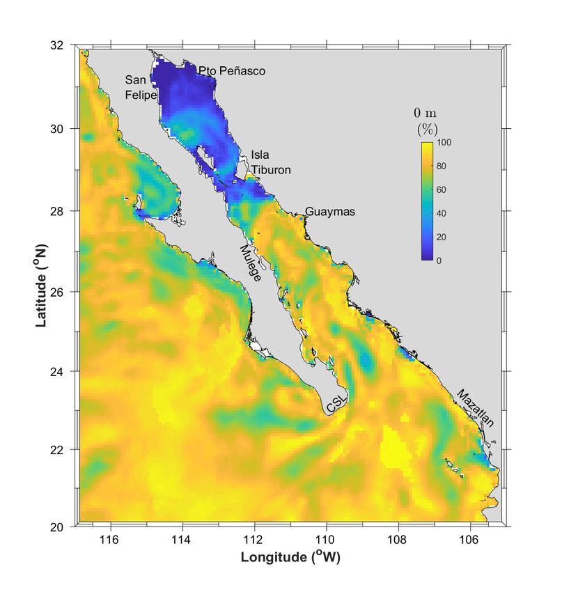
Preprints (www.preprints.org) | NOT PEER-REVIEWED | Posted: 24 February 2020                      doi:10.20944/preprints202002.0216.v2

                           Peer-reviewed version available at Energies 2020, 13, 1095; doi:10.3390/en13051095

                                                                                                                      5 of 18

                   Figure 2. Tidal harmonic reconstruction of the modelled (solid red) and measured (dashed blue) tidal
                   speed m s−1 time series at the SEC mooring, for the same two-week period.


              2.2. Analysis of the barotropic tidal signal
                   The map of U STM , the annual mean of the spring tide maxima, is shown in Fig. 4. The map shows
              two regions with U STM values close to 1 m s−1 . These two regions define two approximate transects
              that are shown in Fig. 3.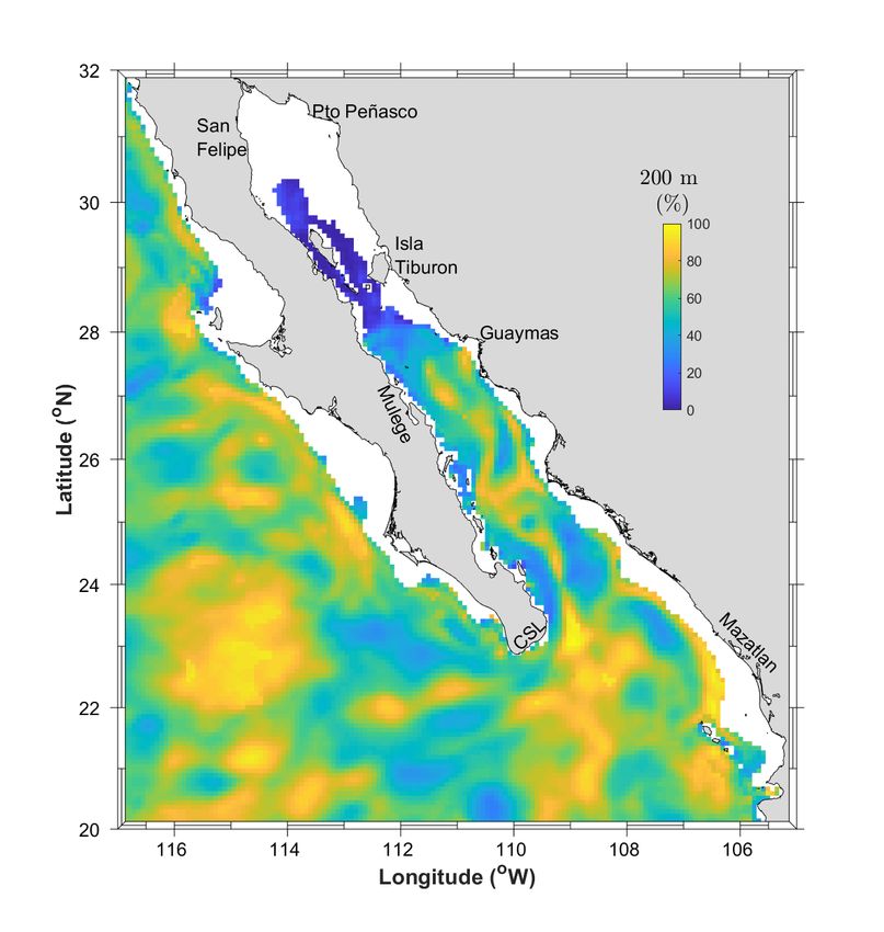
Preprints (www.preprints.org) | NOT PEER-REVIEWED | Posted: 24 February 2020 doi:10.20944/preprints202002.0216.v2
Peer-reviewed version available at Energies 2020, 13, 1095; doi:10.3390/en13051095
6 of 18
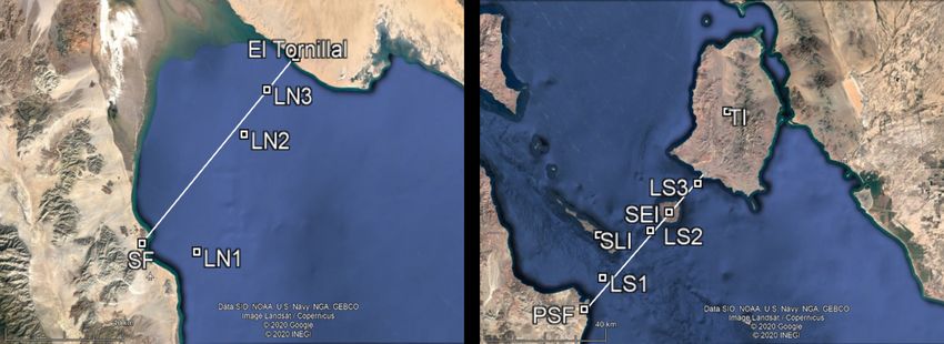
Figure 3. Northern (left) and southern (right) regions with largest tidal current speeds, with
geographical markers for: San Felipe (SF), El Tornillal, Punta San Francisquito (PSF), San Lorenzo
Island (SLI), San Esteban Island (SEI), and Tiburón Island (TI). The six locations with highest tidal
current speeds are also shown.
The first region is in the Upper Gulf of California, in the Colorado River Delta approach in the
North, approximately along a transect running between San Felipe (SF) and El Tornillal, shown on
the left of Fig. 3. The second region is in the GIR, approximately along a transect joining Punta San
Francisquito (PSF) to the western shore of Tiburón Island (TI), shown on the right of Fig. 3. These
landmarks are also shown in the first close-up figure, corresponding to Fig. 5. Now, although most
tidal stream devices operate at mean spring tidal speeds of 2.5 m s−1 or larger, some devices can
operate at locations where spring tidal currents are as low as 1.3 m s−1 [16,17], and where depths are
between 60 m and 120 m. It is possible that such values of U STM are reached in the Upper Gulf or in
the Great Island Region. The location where the model predicts a maximum of Umax is near San Felipe,
and this maximum is of 1.11 m s−1 (see Table 3), which is not far from the minimum threshold of the
GreenDeep device [17]. There are three other location where Umax is above one. However, the model
used here predicts U STM values between 0.8 m s−1 and 0.9 m s−1 . Tidal energy developers need to
design technologies that can exploit lower flow speeds than first generation devices. Higher resolution
models need also to be developed in order to characterize the flow speeds with better spatial detail, in
particular in the GIR.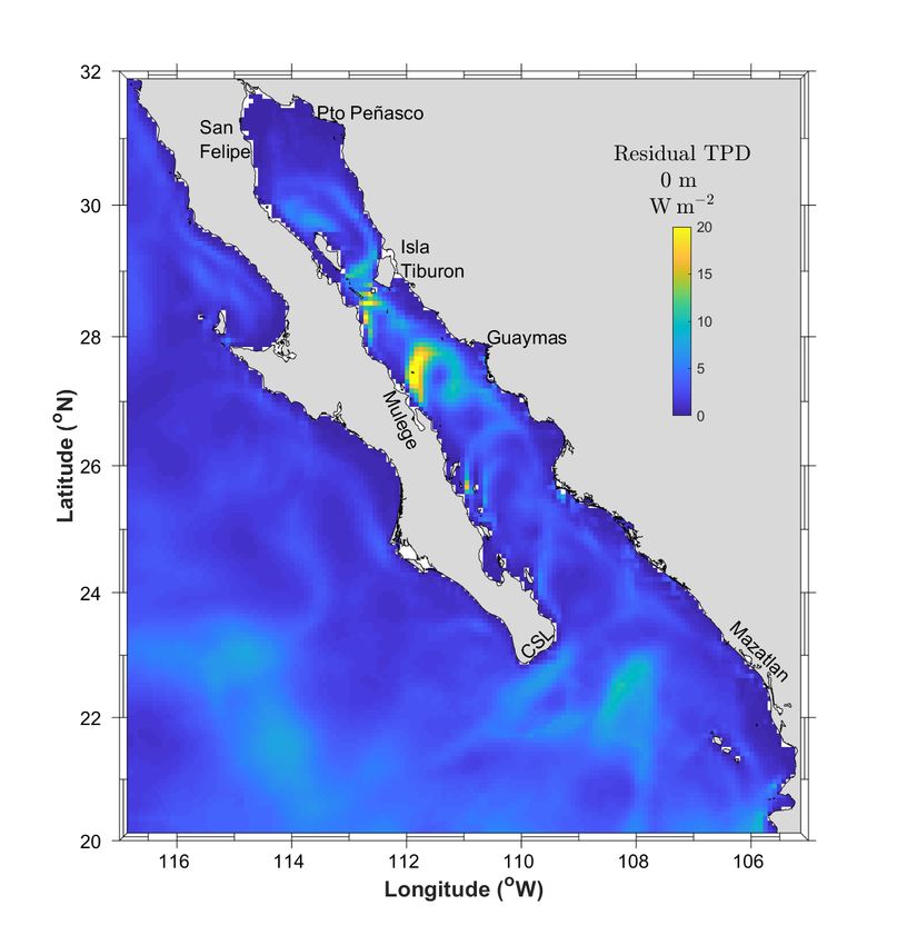
Preprints (www.preprints.org) | NOT PEER-REVIEWED | Posted: 24 February 2020                  doi:10.20944/preprints202002.0216.v2

                         Peer-reviewed version available at Energies 2020, 13, 1095; doi:10.3390/en13051095

                                                                                                                  7 of 18

                              Figure 4. Map of Annual Mean of the Spring Tide Maximum Speed [m s−1 ].

                    Figure 5 shows the regions where TPD reaches values above 50 W m−2 , and the resulting
              annual mean of those values, defined as TPD>50 . We chose 50 W m−2 because it corresponds to
              a minimum threshold speed, Um of 0.46 m s−1 , which is roughly the minimum speed at which
              Tidal Energy Converters (TECs) start reacting to the flow and produce energy. Any speeds below
              Um do not contribute to TPD or the AEP. This minimum threshold defines the regions with no
              commercially viable mean tidal power density. Based on the HYCOM model, such non-commercially
              viable regions appear as blank patches in Fig. 5. The model defines a transect that joins (lat
              lon) = (28◦ N 112◦ 450 54.500 W) in the Peninsula to (lat lon) = (28◦ 270 05.700 N 111◦ 410 07.800 W) on
              mainland Sonora, in the Gulf of California. According to the model, any commercially viable regions
              for tidal energy exploitation in the Gulf of California would be located north of this transect. According
              to the model as well, except for the Colorado River Delta Approach, there are very few places with
              water depths below 50 m which are commercially viable. However, as discussed by Magar [18], there
              are some known exploitable locations in the Channel between Tiburón Island and mainland Sonora.
              Therefore, the HYCOM model may serve as a guidance to identify some locations with exploitable
              resources, but has some limitations at shallow water depths, which may only be solved with better
              bathymetric data, and models with higher resolution. It may be noted that the only location in the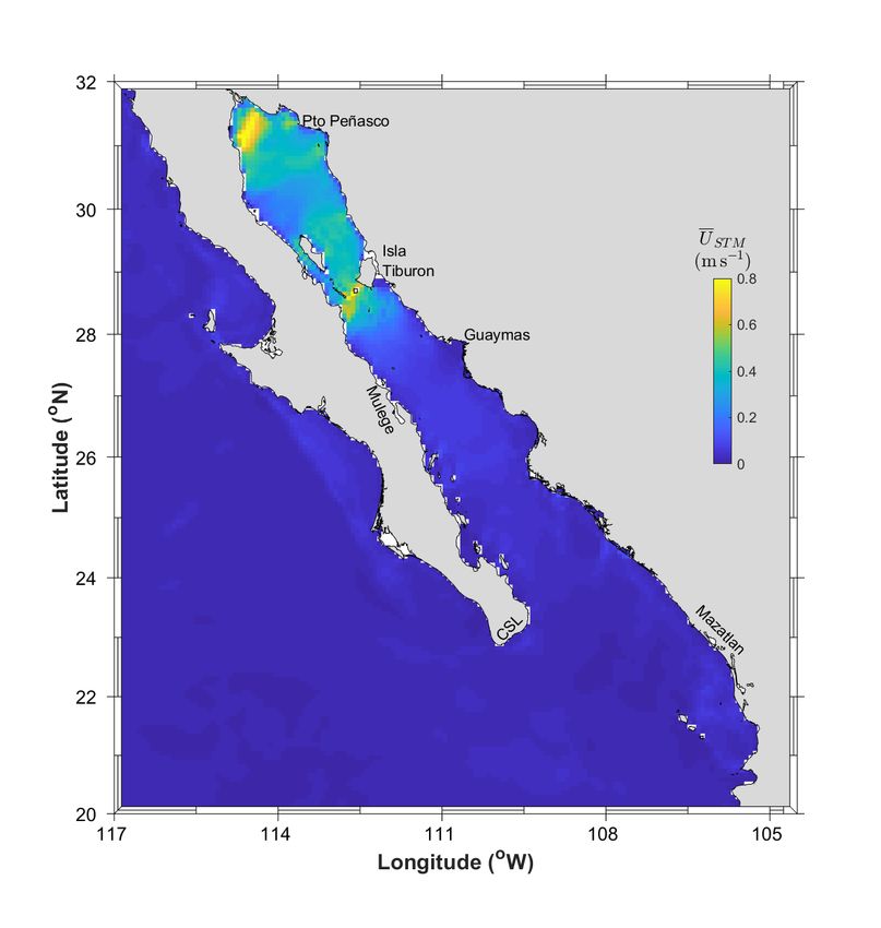
Preprints (www.preprints.org) | NOT PEER-REVIEWED | Posted: 24 February 2020                    doi:10.20944/preprints202002.0216.v2

                          Peer-reviewed version available at Energies 2020, 13, 1095; doi:10.3390/en13051095

                                                                                                                    8 of 18

              Baja Californian Pacific that may have exploitable tidal energy resources, would be the channel just
              north of Punta Eugenia (shown in Fig. 5), as the small colored area in the Baja Californian Pacific coast
              suggests. However, the sites along this coast will not be discussed further in this paper.

                         Figure 5. Map of TPD>50 , corresponding to the mean of TPD when TPD > 50 W m−2 .

                   Figure 6 shows the percentage time (%T) when TPD > 50 W m−2 . The best locations in terms of
              percentage time would correspond to those with largest %T. Along the San Francisquito − Tiburón
              Island transect (the southern transect), the three most relevant locations are LS1, LS2 and LS3 (ordered
              from west to east), their details are in Table 3. Along the San Felipe − El Tornillal transect (the northern
              transect), the three most relevant locations are LN1, LN2 and LN3 (ordered from west to east), their
              details are summarized in Table 3. These six locations are highlighted as void circles in Fig. 6.
Preprints (www.preprints.org) | NOT PEER-REVIEWED | Posted: 24 February 2020 doi:10.20944/preprints202002.0216.v2
Peer-reviewed version available at Energies 2020, 13, 1095; doi:10.3390/en13051095
9 of 18
Table 3. Locations with largest six maximal speeds, Umax , over the simulation year.
h i
Units: U m s−1 and TPD W m−2
Location (lat lon) U STM %T TPD >50 Umax
LN1 (31.006 -114.64) 0.899 39.00 172.8 1.11
LN2 (31.348 -114.48) 0.800 33.58 145.1 1.02
LN3 (31.480 -114.40) 0.758 31.1 141.62 1.02
LS1 (28.506 -112.80) 0.733 23.54 106.7 0.89
LS2 (28.646 -112.64) 0.858 33.34 145.1 1.04
LS3 (28.786 -112.48) 0.676 17.30 92.94 0.83
In terms of barotropic mean tidal power density, the two transects that we have identified are
very similar, with slightly lower TPD>50 values in the southern transect compared to the northern one.
However, the tidal range, the water depth, and the characteristics of the seafloor are distinctly different.
The southern transect changes drastically from very shallow to depths of several hundred meters, has
a seafloor composed of sand and rocks [19], and the tidal range is mostly below 2 m (check the tidal
charts produced by CICESE for the tidal gauges in the GIR, by consulting: http://predmar.cicese.mx/).
In contrast, the northern transect is macrotidal and with water depths mostly below 50 m, with seafloor
composed of cohesive and sandy sediments, and a tidal range that can reach around 6 to 7 m [20,21].
The difference in water depths and seabed sediment composition has important implications on
the type of TEC that can be installed. In particular, the TEC moorings would need to be designed
differently, and a detailed bathymetry would need to be generated in order to find the locations with
depths that are appropriate for deployment. This is not in any way a limitation of the sites, but
an opportunity for device and device deployment innovation [22], from 2nd (Gen2) to 5th (Gen5)
Generation tidal turbine systems [23], and for local scale site characterization studies [24].Preprints (www.preprints.org) | NOT PEER-REVIEWED | Posted: 24 February 2020 doi:10.20944/preprints202002.0216.v2
Peer-reviewed version available at Energies 2020, 13, 1095; doi:10.3390/en13051095
10 of 18
Figure 6. Map of percentage time %T when TPD > 50 W m−2 . The red circles correspond to the six
most energetic locations, defined in the text.
Figure 6 shows the percentage time, %T, when the barotropic TPD is above 50 W m−2 , within
the Gulf of California and for latitudes above the 28◦ parallel. The two transects that have been
discussed previously stand out significantly in Fig. 6, in particular the locations along these transects
with TPD>50 above 140 W m−2 . The most energetic cells are LN1 near San Felipe in the northern
transect, where TPD>50 = 172.8 W m−2 , and LS2 and LN2, where TPD>50 = 145.1 W m−2 . LS2 is
between San Esteban Island (SEI) and San Lorenzo Island (SLI) - shown on the left of Fig. 3, and LN2
is approximately midway between San Felipe and El Tornillal, in the Upper Gulf – shown on the right
of Fig. 3. At these three locations, the %T when TPD > 50 W m−2 is above to 30%.
Figure 7 shows the tidal AEP when considering only values of TPD above 50 W m−2 . In the
regions where production is largest (in the region closest to San Felipe), we reach AEP values of
592 kWh m−2 yr−1 . One tidal stream device with a cross-section diameter of 20 m, or a cross-sectional
area of A = 314.16 m2 ,and an efficiency C p of 0.35 [25,26], would produce a technical AEP of around
65 MWh yr−1 . A Mexican household requires an average of 1.7 to 3.9 MWh yr−1 [27], depending on
their consumption habits, so one device may supply enough energy for 16 to 38 households. In order to
produce a minimum of 1.0 TWh yr−1 , a minimum of 15 devices with a 20 m diameter and an efficiencyPreprints (www.preprints.org) | NOT PEER-REVIEWED | Posted: 24 February 2020 doi:10.20944/preprints202002.0216.v2
Peer-reviewed version available at Energies 2020, 13, 1095; doi:10.3390/en13051095
11 of 18
of at least 35% would be required, conservatively providing enough energy for 240 to 570 households.
As the coastal regions are mostly rural, and with poor transmission line development [28], the energy
produced should be consumed locally, to reduce costs. A tidal farm with 15 devices would be large
enough for that purpose, but it would need to be combined with other energy sources and with energy
storage systems.
Figure 7. Map of AEP when TPD > 50 W m−2 .
2.3. Analysis of the wind-driven in-stream energy resource contribution
The plots in Fig. 8 show the residual TPD at 0 m, 60 m, 100 m, and 200 m below Mean Sea Level.
This residual TPD is linked to the wind-driven currents generated by the Navy Global Environmental
Model (NAVGEM) forcing. The plots show a region between Mulegé and Guaymas, another region
near the southern tip of the Baja California Peninsula, and some locations along the southern transect,
joining San Francisquito to Tiburón Island (identified in the barotropic tides analysis), where TPD ≈
20 W m−2 . From the plots in 8, we deduce that the TPD due to the wind forcing is either around or
less than 20 W m−2 . This is much lower than the economically viable threshold of 50 W m−2 assumed
earlier. Therefore, these TPD values are on their own too low for energy generation, but in locationsPreprints (www.preprints.org) | NOT PEER-REVIEWED | Posted: 24 February 2020 doi:10.20944/preprints202002.0216.v2
Peer-reviewed version available at Energies 2020, 13, 1095; doi:10.3390/en13051095
12 of 18
where tidal currents are strong, such as in the Punta San Francisquito to Tiburón Island transect, they
may play some role in enhancing the tidal energy densities and the annual energy production.
Figure 8. Residual TPD at (a) 0 m, (b) 60 m, (c) 100 m, and (d) 200 m below Mean Sea Level.
Finally, the plots in Fig. 9 show the relative importance of the AEP produced by the wind-driven
currents in relation to the total AEP. The areas where the contribution of the wind-driven current
to the total AEP is really small are also areas with large in-stream tidal energy resources, and where
discussed in Sec. 2.2. The AEP is dominated by the wind-driven component almost everywhere south
of the 28◦ parallel, except for the region in the Baja Californian Pacific that was briefly mentioned at the
end of Sec. 2.2. As the annual TPD is less than 20 W m−2 , it is not large enough to produce energy by
itself. Therefore, the results indicate that the locations for best in-stream energy resource exploitation
are still the two transects identified in Sec. 2.2.Preprints (www.preprints.org) | NOT PEER-REVIEWED | Posted: 24 February 2020 doi:10.20944/preprints202002.0216.v2
Peer-reviewed version available at Energies 2020, 13, 1095; doi:10.3390/en13051095
13 of 18
Figure 9. Relative importance of residual AEP against total AEP at 0 m, 60 m, 100 m, and 200 m below
Mean Sea Level.
3. Materials and Methods
The “Hybrid Coordinate Ocean Model”, referred to as HYCOM since its inception [29], was
developed as an outgrowth of the “Miami Isopycnic Coordinate Ocean Model”, or MICOM, described
in Bleck et al. [30]. The model is a primitive equation model with two prognostic equations for the
horizontal velocity components (which we express in terms of the velocity vector), one representing
the mass continuity or layer-thickness tendency, one for salinity and one for temperature.
The HYCOM experiment we used employs atmospheric forcing from the Navy Global
Environmental Model (NAVGEM) [31], and geopotential tidal forcing from the five largest principal
tidal components: M2 , S2 , N2 , K1 and O1 . A self-attraction and load (SAL) term is added to the
tidal forcing. The SAL term accounts for the self-gravitation of the tidally deformed ocean and solid
earth [32], and for the load deformations of the solid earth [33]. The model has a nominal horizontal
resolution of 1/12.5◦ at the equator and 41 isopycnal layers in the vertical. The NAVGEM has aPreprints (www.preprints.org) | NOT PEER-REVIEWED | Posted: 24 February 2020 doi:10.20944/preprints202002.0216.v2
Peer-reviewed version available at Energies 2020, 13, 1095; doi:10.3390/en13051095
14 of 18
horizontal resolution of 0.33◦ , and is interpolated to the finer resolution of the hydrodynamic grid
for the simulations. First, the model is run from 1996 to 2003 with a climatological forcing, then from
2003 to 2011 with the atmospheric forcing from the Navy Operational Global Atmospheric Prediction
System, NOGAPS [34], and finally, the atmospheric NAVGEM forcing is applied after 30 June 2011.
Tidal forcing is initiated on 3 July 2011. Global three-dimensional fields are stored every hour for one
year, from 1 October 2011 to 1 October 2012. More details can be found in [3,4].
The analysis is performed over the domain and with the bathymetry shown in Fig. 1, which is
the ETOPO1 bathymetry with some sounding corrections in the Great Island Region (GIR) courtesy
of CICESE (Zamudio, pers. comm.), described in [35]. The GIR moorings were deployed during the
“umbrales” (2002-2006) project; these moorings were first reported in [36,37]. The ISJ mooring was
deployed between June 2017 and November 2017 during the “CeMIE-Océano” (2017-2021) project,
and was first reported in [38].
The in-situ data mentioned above were used to verify the model predictions in the GIR and in
ISJ. Since the modelling period extended between 01/10/2011 01:00:00 and 01/10/2012 00:00:00 in
hourly timesteps, but the ADCP data were collected at different periods, the verification analysis of
the model against the data was performed for the period modelled in the simulations, and focused on
the depth-averaged tidal signal alone. The tidal principal component analyses for the ADCP and the
simulation results were performed with the T_TIDE tidal analysis package [2], and the tidal signal was
reconstructed from the tidal principal components for the simulation period. From this reconstruction,
we computed the annual mean tidal speed U, the annual mean tidal power density TPD, and the
annual energy power AEP:
N
1
U =
N ∑ Ui , (1)
i =1
N
1
TPD = ρ ∑ Ui3 , and (2)
2N i=1
1 N 3
2 i∑
AEP = ρ Ui , (3)
=1
q
with Ui = u2i + v2i , N = 8784 (2012 is a leap year), and ρ = 1024 kg m−3 is the water density. U, TPD,
and AEP are computed for the model (mod) and the mooring (obs) data, at each mooring location.
The agreement between model X = xmod and observation Y = xobs was assessed using the
Pearson correlation coefficient, ρ X,Y , defined as [39]:
cov( X, Y )
ρ X,Y = , (4)
σX σY
where cov is the covariance between the two time series, and σX and σY the standard deviations
of X and Y, respectively; the relative error REx ,
x obs − x mod
REx = ; (5)
x obs
and the root mean square error RMSEx ,
v
N
u
u1
RMSEx = t
N ∑ (xi,obs − xi,mod )2 , (6)
i =1
over the simulation period. Once the model was validated at the mooring locations, we analysed
the field maps of U, TPD, and AEP, as well as the annual means of the spring tide maxima, U STM and
TPD STM , to determine the best sites for tidal and wind-driven current energy extraction, based on
U, TPD, and AEP. We also assessed the percentage contribution of each of them throughout the casePreprints (www.preprints.org) | NOT PEER-REVIEWED | Posted: 24 February 2020 doi:10.20944/preprints202002.0216.v2
Peer-reviewed version available at Energies 2020, 13, 1095; doi:10.3390/en13051095
15 of 18
study domain, and discuss some implications for tidal and wind-driven current power generation. It
is worth noting that here we will not consider any techo-economic or socio-ecological constraints, but
the analysis would be similar to that for wind energy resource characterization studies developed in
previous work [28,40].
4. Conclusions
Data from a global HYCOM model with tide and wind forcings and no data assimilation was
used to make a mesoscale evaluation of in-stream renewable energy resources in the Gulf of California
and the Baja Californian Pacific. Specifically, the model was used to separate and analyze the tidal and
wind-driven current speeds, tidal power densities, and annual energy production in the region. The
model showed there are two areas within the Gulf of California, one in the Great Island Region and one
in the Upper Gulf of California, with mean annual tidal power densities between 141 and 173 W m−2 .
At some locations in these areas, energy would be produced for around 31% to 39% of the year, with
technologies that can generate electricity above a minimum speed threshold of 0.46 m s−1 , equivalent
to a minimum TDP threshold of 50 W m−2 . The in-stream energy resources are strongly dominated by
the tidal stream component, with wind-driven current speeds associated with TPDs generally below
20 W m−2 , which is below the minimum TPD threshold for energy generation. The installation of 15
devices with a diameter of 20 m and an efficiency of 35% would provide enough energy for 240 to
570 households. These devices could be installed along two transects, either between San Felipe and
El Tornillal in the Upper Gulf of California, or between San Francisquito and Tiburón Island, in the
Great Island Region. Subsequent studies may either assess the suitability for marine renewable energy
developments from a socio-economic perspective, or improve the speeds, TPD and AEP assessments
by using a model with higher spatial resolution at the two relevant transects identified in this paper.
Author Contributions: conceptualization, VM and MSG; methodology, VM and LZ; software, LZ; validation,
MLM and VMG; formal analysis, VM; data curation, ABR, MLM and VMG; resources, JC; writing–original draft
preparation, VM; writing–review and editing, all authors; visualization, VMG and VM; project administration,
VM; funding acquisition, VM.
Funding: This work was partially supported by the SENER-CONACYT grant no. 249795, within the project
“CeMIE-Océano” (2017-2021).
Acknowledgments: Thanks to the Department of Physical Oceanography of CICESE, and in particular technician
Erick Rivera-Lemus, for his support with fieldwork and data acquisition. Thanks to the waves group of CICESE
(led by Dr. Paco Ocampo), for support with technician time and batteries provided for instrumentation. Thanks
to the Oceanographic Equipment Coordination and the CANEK group of CICESE, for support with equipment
and equipment maintenance resources. HYCOM simulation was performed on the Navy Department of Defense
(DoD) Supercomputing Resources at Stennis Space Center, Mississippi, using grants of computer time from
the DoD High Performance Computing Modernization Program. Thanks to the anonymous reviewers for their
comments.
Conflicts of Interest: The authors declare no conflict of interest. The funders had no role in the design of the
study; in the collection, analyses, or interpretation of data; in the writing of the manuscript, or in the decision to
publish the results.
AbbreviationsPreprints (www.preprints.org) | NOT PEER-REVIEWED | Posted: 24 February 2020 doi:10.20944/preprints202002.0216.v2
Peer-reviewed version available at Energies 2020, 13, 1095; doi:10.3390/en13051095
16 of 18
The following abbreviations are used in this manuscript:
ADCP Acoustic Doppler Current Profiler
AEP Annual Energy Production
BC Ballenas Channel
DS Delfin Sill
ETOPO1 Earth topography and bathymetry global relief model, at 1 arc-minute resolution
GIR Great Island Region
HYCOM Hybrid Coordinate Ocean Model
ISJ Isla San Jorge
LN Location North
LS Location South
MICOM Miami Isopycnic Coordinate Ocean Model
MRE Marine Renewable Energy
MUPS Multi-Use Platforms at Sea
NAVGEM Navy Global Environmental Model
NOGAPS Navy Operational Global Atmospheric Prediction System
PSF Punta San Francisquito
SAL self-attraction and load
SEC San Esteban Channel
SF San Felipe
SLC San Lorenzo Channel
TI Tiburón Island
TPD Tidal Power Density
T_TIDE Tidal Harmonic Analysis Toolbox
References
1. Parker, B.B., Ed. Tidal Hydrodynamics; Wiley, 1991.
2. Pawlowicz, R.; Beardsley, B.; Lentz, S. Classical tidal harmonic analysis including error estimates in
MATLAB using T_TIDE. Computers & Geosciences 2002, 28, 929–937. doi:10.1016/s0098-3004(02)00013-4.
3. Buijsman, M.C.; Arbic, B.K.; Richman, J.G.; Shriver, J.F.; Wallcraft, A.J.; Zamudio, L. Semidiurnal internal
tide incoherence in the equatorial Pacific. Journal of Geophysical Research: Oceans 2017, 122, 5286–5305.
doi:10.1002/2016jc012590.
4. Arbic, B.K.; Alford, M.H.; Ansong, J.K.; Buijsman, M.C.; Ciotti, R.B.; Farrar, J.T.; Hallberg, R.W.; Henze, C.E.;
Hill, C.N.; Luecke, C.A.; Menemenlis, D.; Metzger, E.J.; Müeller, M.; Nelson, A.D.; Nelson, B.C.; Ngodock,
H.E.; Ponte, R.M.; Richman, J.G.; Savage, A.C.; Scott, R.B.; Shriver, J.F.; Simmons, H.L.; Souopgui, I.; Timko,
P.G.; Wallcraft, A.J.; Zamudio, L.; Zhao, Z. A Primer on Global Internal Tide and Internal Gravity Wave
Continuum Modeling in HYCOM and MITgcm. In New Frontiers in Operational Oceanography; GODAE
OceanView, 2018. doi:10.17125/gov2018.ch13.
5. Gross, M.; Magar, V. Wind-Induced Currents in the Gulf of California from Extreme Events and
Their Impact on Tidal Energy Devices. Journal of Marine Science and Engineering 2020, 8, 80.
doi:10.3390/jmse8020080.
6. Dupont, F.; Hannah, C.G.; Greenberg, D. Modelling the sea level of the upper Bay of Fundy.
Atmosphere-Ocean 2005, 43, 33–47. doi:10.3137/ao.430103.
7. Hiriart Le Bert, G. Potencial energético del Alto Golfo de California. Boletín de la Sociedad Geológica Mexicana
2009, 61, 143–146. doi:10.18268/bsgm2009v61n1a13.
8. Xia, J.; Falconer, R.A.; Lin, B. Hydrodynamic impact of a tidal barrage in the Severn Estuary, UK. Renewable
Energy 2010, 35, 1455–1468. doi:10.1016/j.renene.2009.12.009.
9. Carbajal, N.; Backhaus, J.O. Simulation of tides, residual flow and energy budget in the Gulf of California.
Oceanologica Acta 1998, 21, 429–446. doi:10.1016/s0399-1784(98)80028-5.
10. Garrett, C.; Cummins, P. The power potential of tidal currents in channels. Proceedings of the Royal Society
A: Mathematical, Physical and Engineering Sciences 2005, 461, 2563–2572. doi:10.1098/rspa.2005.1494.Preprints (www.preprints.org) | NOT PEER-REVIEWED | Posted: 24 February 2020 doi:10.20944/preprints202002.0216.v2
Peer-reviewed version available at Energies 2020, 13, 1095; doi:10.3390/en13051095
17 of 18
11. Defne, Z.; Haas, K.A.; Fritz, H.M. Numerical modeling of tidal currents and the effects of power
extraction on estuarine hydrodynamics along the Georgia coast, USA. Renewable Energy 2011, 36, 3461–3471.
doi:10.1016/j.renene.2011.05.027.
12. Yang, X.; Haas, K.A.; Fritz, H.M. Theoretical Assessment of Ocean Current Energy Potential for the Gulf
Stream System. Marine Technology Society Journal 2013, 47, 101–112. doi:10.4031/mtsj.47.4.3.
13. Perez-Collazo, C.; Pemberton, R.; Greaves, D.; Iglesias, G. Monopile-mounted wave energy
converter for a hybrid wind-wave system. Energy Conversion and Management 2019, 199, 111971.
doi:10.1016/j.enconman.2019.111971.
14. Stuiver, M.; Soma, K.; Koundouri, P.; van den Burg, S.; Gerritsen, A.; Harkamp, T.; Dalsgaard, N.; Zagonari,
F.; Guanche, R.; Schouten, J.J.; Hommes, S.; Giannouli, A.; Söderqvist, T.; Rosen, L.; Garção, R.; Norrman,
J.; Röckmann, C.; de Bel, M.; Zanuttigh, B.; Petersen, O.; Møhlenberg, F. The Governance of Multi-Use
Platforms at Sea for Energy Production and Aquaculture: Challenges for Policy Makers in European Seas.
Sustainability 2016, 8, 333. doi:10.3390/su8040333.
15. Dalton, G.; Bardócz, T.; Blanch, M.; Campbell, D.; Johnson, K.; Lawrence, G.; Lilas, T.; Friis-Madsen, E.;
Neumann, F.; Nikitas, N.; Ortega, S.T.; Pletsas, D.; Simal, P.D.; Sørensen, H.C.; Stefanakou, A.; Masters, I.
Feasibility of investment in Blue Growth multiple-use of space and multi-use platform projects; results of a
novel assessment approach and case studies. Renewable and Sustainable Energy Reviews 2019, 107, 338–359.
doi:10.1016/j.rser.2019.01.060.
16. Tweed, K. Underwater Kite Harvests Energy From Slow Currents – Could kites be the secret to capturing
tidal energy?, 2013. Last accessed: 19/11/2019.
17. Minesto. https://www.minesto.com/our-technology, 2019. Last accessed: 19/11/2019.
18. Magar, V. Tidal Current Technologies. In Sustainable Energy Technologies; CRC Press, 2017; pp. 293–308.
doi:10.1201/9781315269979-18.
19. Byrne, J.V.; Emery, K.O. Sediments of the Gulf of California. Geological Society of America Bulletin 1960,
71, 983. doi:10.1130/0016-7606(1960)71[983:sotgoc]2.0.co;2.
20. Morales Pérez, R.A.; Gutiérrez de Velazco Sanromán, G. Mareas en el Golfo de California. Geofísica
Internacional 1989, 28, 25 – 46.
21. Álvarez, L.G.; Suárez-Vidal, F.; Mendoza-Borunda, R.; González-Escobar, M. Bathymetry and active
geological structures in the Upper Gulf of California. Boletín de la Sociedad Geológica Mexicana 2009, 61, 129 –
141.
22. Corsatea, T.D.; Magagna, D. Overview of European innovation activities in marine energy technology.
Technical report, Environmental Sciences Group, Brussels, BE, 2014.
23. Verdant Power. Technology Advancement, 2019. Last accessed: 21/11/2019.
24. LeGrand, C. Assessment of Tidal Energy Resource – Marine Renewable Energy Guides. Technical report,
Black and Veatch Ltd, London, UK, 2009.
25. Myers, L.; Bahaj, A. Power output performance characteristics of a horizontal axis marine current turbine.
Renewable Energy 2006, 31, 197–208. doi:10.1016/j.renene.2005.08.022.
26. Iyer, A.; Couch, S.; Harrison, G.; Wallace, A. Variability and phasing of tidal current energy around the
United Kingdom. Renewable Energy 2013, 51, 343–357. doi:10.1016/j.renene.2012.09.017.
27. Oropeza-Perez, I.; Petzold-Rodriguez, A. Analysis of the Energy Use in the Mexican Residential Sector
by Using Two Approaches Regarding the Behavior of the Occupants. Applied Sciences 2018, 8, 2136.
doi:10.3390/app8112136.
28. Magar, V.; Gross, M.; González-García, L. Offshore wind energy resource assessment under
techno-economic and social-ecological constraints. Ocean & Coastal Management 2018, 152, 77–87.
doi:10.1016/j.ocecoaman.2017.10.007.
29. Bleck, R. An oceanic general circulation model framed in hybrid isopycnic-Cartesian coordinates. Ocean
Modelling 2002, 4, 55–88. doi:10.1016/s1463-5003(01)00012-9.
30. Bleck, R.; Rooth, C.; Hu, D.; Smith, L.T. Salinity-driven Thermocline Transients in a Wind- and
Thermohaline-forced Isopycnic Coordinate Model of the North Atlantic. Journal of Physical Oceanography
1992, 22, 1486–1505. doi:10.1175/1520-0485(1992)0222.0.co;2.
31. Hogan, T.F.; Liu, M.; Ridout, J.A.; Peng, M.S.; Whitcomb, T.R.; Ruston, B.C.; Reynolds, C.A.; Eckermann,
S.D.; Moskaitis, J.R.; Baker, N.L.; McCormack, J.P.; Viner, K.C.; Mclay, J.G.; Flatau, M.K.; Xu, L.; Chen, C.;
Chang, S.W. The Navy Global Environmental Model. Oceanography 2014, 27, 116–125.Preprints (www.preprints.org) | NOT PEER-REVIEWED | Posted: 24 February 2020 doi:10.20944/preprints202002.0216.v2
Peer-reviewed version available at Energies 2020, 13, 1095; doi:10.3390/en13051095
18 of 18
32. Ray, R.D. Ocean self-attraction and loading in numerical tidal models. Marine Geodesy 1998, 21, 181–192.
doi:10.1080/01490419809388134.
33. Hendershott, M.C. The Effects of Solid Earth Deformation on Global Ocean Tides. Geophysical Journal
International 1972, 29, 389–402. doi:10.1111/j.1365-246x.1972.tb06167.x.
34. Rosmond, T.; Teixeira, J.; Peng, M.; Hogan, T.; Pauley, R. Navy Operational Global Atmospheric
Prediction System (NOGAPS): Forcing for Ocean Models. Oceanography 2002, 15, 99–108.
doi:10.5670/oceanog.2002.40.
35. Argote, M.L.; Amador, A.; Lavín, M.F.; Hunter, J.R. Tidal dissipation and stratification in the Gulf of
California. Journal of Geophysical Research 1995, 100, 16103. doi:10.1029/95jc01500.
36. López, M.; Candela, J.; Argote, M.L. Why does the Ballenas Channel have the coldest SST in the Gulf of
California? Geophysical Research Letters 2006, 33. doi:10.1029/2006gl025908.
37. López, M.; Candela, J.; García, J. Two overflows in the Northern Gulf of California. Journal of Geophysical
Research 2008, 113. doi:10.1029/2007jc004575.
38. Bermúdez-Romero, A.; Magar, V.; Gross, M.S.; Godínez, V.M.; López-Mariscal, M.; Rivera-Lemus, E.
Characterization of in-stream tidal energy resources in the Gulf of California: implementation, calibration
and validation of a hydrodynamic model. Proceedings of the 13th European Wave and Tidal Energy
Conference (EWTEC2019), Napoli, Italy, 2019, European Wave and Tidal Energy Conference Series.
39. Pearson, K. Mathematical Contributions to the Theory of Evolution. III. Regression, Heredity, and
Panmixia. Philosophical Transactions of the Royal Society A: Mathematical, Physical and Engineering Sciences
1896, 187, 253–318. doi:10.1098/rsta.1896.0007.
40. Magar, V.; González-García, L.; Gross, M.S. Evaluación Técnico-económica del Potencial de
Desarrollo de Parques Eólicos en Mar: El Caso del Golfo de California. BIOtecnia 2017, 19, 3–8.
doi:10.18633/biotecnia.v19i0.358.You can also read