Implementing a sectional scheme for early aerosol growth from new particle formation in the Norwegian Earth System Model v2: comparison to ...
←
→
Page content transcription
If your browser does not render page correctly, please read the page content below
Geosci. Model Dev., 14, 3335–3359, 2021
https://doi.org/10.5194/gmd-14-3335-2021
© Author(s) 2021. This work is distributed under
the Creative Commons Attribution 4.0 License.

Implementing a sectional scheme for early aerosol growth from new
particle formation in the Norwegian Earth System Model v2:
comparison to observations and climate impacts
Sara M. Blichner1 , Moa K. Sporre2 , Risto Makkonen3,4 , and Terje K. Berntsen1
1 Department    of Geosciences and Centre for Biogeochemistry in the Anthropocene, University of Oslo, Oslo, Norway
2 Department    of Physics, Lund University, Lund, Sweden
3 Institute for Atmospheric and Earth System Research/Physics, Faculty of Science, University of Helsinki,

Helsinki, Finland
4 Climate System Research, Finnish Meteorological Institute, Helsinki, Finland

Correspondence: Sara Marie Blichner (s.m.blichner@geo.uio.no)

Received: 21 October 2020 – Discussion started: 12 November 2020
Revised: 16 March 2021 – Accepted: 1 April 2021 – Published: 4 June 2021

Abstract. Aerosol–cloud interactions contribute to a large      duces much fewer particles than the original scheme in pol-
portion of the spread in estimates of climate forcing, cli-     luted regions, while it produces more in remote regions and
mate sensitivity and future projections. An important part of   the free troposphere, indicating a potential impact on the
this uncertainty is how much new particle formation (NPF)       estimated aerosol forcing. Finally, we analyse the effect on
contributes to cloud condensation nuclei (CCN) and, further-    cloud–aerosol interactions and find that the effect of changes
more, how this changes with changes in anthropogenic emis-      in NPF efficiency on clouds is highly heterogeneous in space.
sions. Incorporating NPF and early growth in Earth system       While in remote regions, more efficient NPF leads to higher
models (ESMs) is, however, challenging due to uncertain pa-     cloud droplet number concentration (CDNC), in polluted re-
rameters (e.g. participating vapours), structural issues (nu-   gions the opposite is in fact the case.
merical description of growth from ∼ 1 to ∼ 100 nm) and
the large scale of an ESM grid compared to the NPF scale. A
common approach in ESMs is to represent the particle size
distribution by a certain number of log-normal modes. Sec-      1   Introduction
tional schemes, on the other hand, in which the size distri-
bution is represented by bins, are considered closer to first   The formation of new particles in the atmosphere, known as
principles because they do not make an a priori assumption      new particle formation (NPF), occurs through the clustering
about the size distribution.                                    and nucleation of low-volatility vapours. These particles can
   In order to improve the representation of early growth, we   then influence the climate by growing via condensation to
have implemented a sectional scheme for the smallest par-       sizes at which they act as cloud condensation nuclei (CCN)
ticles (5–39.6 nm diameter) in the Norwegian Earth System       (Twomey, 1974; Albrecht, 1989) – or even by interacting
Model (NorESM), feeding particles into the original aerosol     directly with radiation if they grow large enough (Boucher
scheme. This is, to our knowledge, the first time such an ap-   et al., 2013). NPF has received increasing attention in re-
proach has been tried. We find that including the sectional     cent years due to the aforementioned climate impacts as well
scheme for early growth improves the aerosol number con-        as its implications for human health. This has lead to new
centration in the model when comparing against observa-         insights into the mechanisms involved in NPF, and subse-
tions, particularly in the 50–100 nm diameter range. Further-   quently new parameterization schemes have been developed
more, we find that the model with the sectional scheme pro-     and included in Earth system models (ESMs). For example,
                                                                Gordon et al. (2016) showed that including a NPF pathways

Published by Copernicus Publications on behalf of the European Geosciences Union.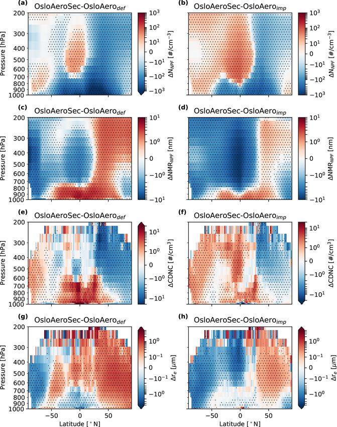
3336       S. M. Blichner et al.: Implementing a sectional scheme for early aerosol growth from new particle formation

from pure organic nucleation nucleation (Kirkby et al., 2016;       crease in both condensation and coagulation sink, which fur-
Riccobono et al., 2014; Gordon et al., 2017, 2016; Dunne            ther decreases the growth rate and increases the coagulation
et al., 2016; Tröstl et al., 2016) in a global aerosol model re-    sink of new particles forming. The result is then a suppres-
sulted in a considerable diminishing of the estimated negative      sion of further NPF (e.g. Westervelt et al., 2014, 2013; Se-
forcing due to aerosol–cloud interactions since pre-industrial      meniuk and Dastoor, 2018; Carslaw et al., 2013; Kerminen
times (+0.22 W m−2 , 27 %). This result illustrates the impor-      et al., 2018; Schutgens and Stier, 2014). These loss processes
tance of adequately representing the effects of NPF in ESMs         which constrain the survival of new particles to larger sizes
for our understanding of historical forcing and thus climate        may in fact often be more important than the nucleation rate
sensitivity, especially considering that cloud–aerosol interac-     in itself. For example, Carslaw et al. (2013) show that the
tions are estimated to be responsible for a large fraction of the   Global Model of Aerosol Processes (GLOMAP) has low sen-
observed negative radiative forcing since pre-industrial times      sitivity for particles larger than 50 nm to nucleation rate pa-
(Boucher et al., 2013).                                             rameterizations but high sensitivity to processes affecting the
   In spite of NPF being the subject of a lot of research over      coagulation loss of newly formed particles. This underlines
recent years, there is still uncertainty about the species in-      the importance of adequately representing the processes that
volved in both nucleation and subsequent particle growth            constrain the formation of new particles. If not we could end
(Kerminen et al., 2018; Lee et al., 2019). In order for NPF         up with models wherein both the aerosol number concentra-
to be successful, particles must form and grow up to a de-          tion and CCN are overly sensitive to changes in emissions.
cent size, often defined to be out of the nucleation mode, i.e.        While there is a large body of work on describing when
10 nm. Due to the Kelvin effect, only atmospheric gases with        NPF happens in many individual environments, the transferal
very low volatility are able to contribute to the initial steps     of this to a generalized context (which is what is needed for
in NPF, and in many atmospheric conditions the growth rates         a climate model) is very uncertain. In other words, based on
provided are too slow for particles to survive losses to coag-      knowledge of what drives NPF in a specific environment it
ulation and evaporation (Semeniuk and Dastoor, 2018). Sul-          is not easy to derive a general parameterization (Kerminen
furic acid is known to be the most important species for nu-        et al., 2018; Lee et al., 2019).
cleation due to its low vapour pressure, while bases such as           From the perspective of an ESM, aerosols only become
amines and ammonia may enhance the nucleation rate (Lee             relevant when they approach ∼ 50 nm in diameter and may,
et al., 2019; Kerminen et al., 2018). There is evidence that        depending on the conditions, act as CCN (Kerminen et al.,
extremely low-volatility organic vapours also contribute sig-       2012). However, because the formation of particles in this
nificantly, especially in remote areas (Semeniuk and Das-           size range is highly dependent on aerosol dynamics at
toor, 2018; Dunne et al., 2016; Riccobono et al., 2014). For        smaller sizes, climate models need to treat these dynamics
the subsequent growth of the particles, the Kelvin effect de-       with a sufficient degree of accuracy. Since climate models
creases and condensing organics of higher volatility, predom-       are required to run hundreds of years of simulations within a
inantly originating from the oxidation of biogenic volatile         reasonable time span, this involves a trade-off between rep-
organic compounds (BVOCs), become more and more dom-                resenting the physical process to the best of our scientific un-
inant and are essential in most environments (Riipinen et al.,      derstanding on one hand and computational cost on the other
2011; Tröstl et al., 2016).                                         hand.
   During all stages of particle growth, the particles are sub-        In ESMs, it is common to use modal schemes to repre-
ject to coagulation, reducing the number of particles that          sent the particle size distribution – i.e. describing the distri-
form and that grow to sizes at which they can act as CCN            bution as the sum of some number of log-normal modes (e.g.
(∼ 50 nm in diameter; Kerminen et al., 2012). The majority          Stier et al., 2005; Liu et al., 2005; Mann et al., 2010; Vignati
of this coagulation will occur with particles that are already      et al., 2004). On the other hand, sectional schemes – in which
in the CCN size range and thus results in a net loss of par-        the size distribution is represented by bins (e.g. Spracklen
ticles that could eventually act as CCN. However, when two          et al., 2005; Kokkola et al., 2008) – are in general consid-
small particles (below the CCN size range) coagulate, this          ered closer to first principles because they do not make an
contributes to growth of the combined particle, which could         a priori assumption about the size distribution. Nevertheless,
then become a cloud condensation nucleus (e.g. Kerminen             modal schemes are generally favoured in ESMs because they
et al., 2018; Lee et al., 2013; Schutgens and Stier, 2014). This    require fewer tracers and are much cheaper computationally.
effect, though, is only significant in highly polluted regions.        Any size-resolving aerosol scheme must have a cut-off
The survival rate of NPF particles to CCN sizes is there-           diameter at which explicit modelling of aerosol number,
fore in general dependent on competition between the par-           growth and losses begins. One natural choice is the size of
ticle growth rate by condensation and the coagulation sink.         the critical cluster, around 1 nm (Lee et al., 2013). While this
   The formation of new particles is tightly constrained by         means that the entire size distribution of particles is treated,
negative feedbacks. If NPF is high, the result will be an in-       it adds disproportionate computational cost to the simulation
crease in particle number and with it an increase in the avail-     for aerosols with a very short atmospheric lifetime (due to
able surface area for condensation. This will lead to an in-        both growth out of the size range and high sensitivity to co-

Geosci. Model Dev., 14, 3335–3359, 2021                                              https://doi.org/10.5194/gmd-14-3335-2021
S. M. Blichner et al.: Implementing a sectional scheme for early aerosol growth from new particle formation                        3337

agulation) (see e.g. Lee et al., 2013). An alternative is to pa-
rameterize the growth and coagulation loss of particles up to
a larger diameter, which is the approach used in most ESMs
(Kerminen and Kulmala, 2002; Kerminen et al., 2004; Lehti-
nen et al., 2007; Anttila et al., 2010). These methods involve
estimating the flux or the formation of particles at the cut-off
diameter, be it modal or sectional, based on estimated growth
rate and coagulation sink (see details in the model descrip-
tion).
   There are several drawbacks of this approach, especially if
the chosen cut-off diameter is high. The most important one
is that it assumes steady state, i.e. the same constant growth
rates from the particle formed up to the cut-off value, which
in reality could take several time steps and long enough for
conditions to change substantially (hours). A particle may
form under conditions with a high growth rate, but in the
time it would take for the particle to grow to the cut-off di-
ameter, the growth rate might decrease due to an increased
condensation sink by the many new particles being formed.          Figure 1. Illustration of changes from OsloAero to OsloAeroSec.
In a model with a relatively high cut-off, this would lead to      In both versions, the nucleation rate is calculated at around 2 nm,
an overestimation of the growth rate of the nucleated parti-       followed by a calculation of the formation rate (the particles surviv-
                                                                   ing) at 5 and 23.6 nm in OsloAeroSec and OsloAero, respectively,
cle, which would in turn lead to an overestimation of the for-
                                                                   with Lehtinen et al. (2007). In OsloAero, these particles are inserted
mation rate at the cut-off (Olenius and Riipinen, 2017; Lee        directly into the modal scheme, while in OsloAeroSec, the particles
et al., 2013). Olenius and Riipinen (2017) test the effect of      are inserted into the sectional scheme wherein they can be affected
the cut-off diameter by explicitly modelling the formation of      by growth and coagulation over time and space. Finally, the par-
particles from vapour molecules to 10 nm diameter and find         ticles in the sectional scheme are moved from the last bin of the
an overprediction by a factor of 2 or even orders of magni-        sectional scheme to the modal scheme. ∗ 23.6 nm is the number me-
tude. Similarly, Lee et al. (2013) suggest that during nucle-      dian diameter of the mode the particles from the sectional scheme
ation events, the smallest particles (< 10 nm) can be a sig-       are moved to, but particles are actually grown to the volume median
nificant condensation sink, thus regulating nucleation via re-     diameter (39.6 nm) before they are moved to the modal scheme in
duced concentrations of precursors. They investigate the ef-       order to conserve mass.
fects of cut-off diameter with a sectional aerosol scheme in
the GISS-TOMAS model and compare a 1 nm cut-off with 3             tion, at which point the air mass may have moved consider-
and 10 nm cut-offs using Kerminen et al. (2004) to parame-         ably. This is in particular the case with a high cut-off value,
terize the survival of nucleated particles to the cut-off. They    like in NorESM (23.6 nm) (Kirkevåg et al., 2018).
find that using a 10 nm cut-off leads to an overestimation of         In order to improve the representation of early parti-
CCN at 0.2 % supersaturation, with 10 %–20 % overestima-           cle growth, we have implemented a sectional scheme for
tion in the surface layer in most of the Northern Hemisphere,      the smallest particles (5–39.6 nm diameter) in the aerosol
while the globally averaged change to CCN(0.2 %) is minor.         scheme in the Norwegian Earth System Model (NorESM).
Furthermore, a 10 nm cut-off produces a high bias in the con-      The sectional scheme acts as an intermediate step during
centration of particles larger than 10 nm (N10 ) of up to a fac-   NPF and feeds the grown particles into the original modal
tor of 3–5 in regions with high nucleation. In addition, they      scheme. This is, to our knowledge, the first time such a hy-
find that the 10 nm cut-off is sensitive to the time step.         brid approach has been attempted. The sectional scheme cur-
   Another drawback of a high cut-off diameter is that most        rently involves two condensing species (sulfuric acid and
of these parameterizations neglect self-coagulation within         low-volatility organics) and five bins. The aerosol scheme
the sub-cut-off size range, which can be an important growth       with these changes will be referred to as OsloAeroSec. A
mechanism during intense new particle formation events.            schematic of the changes from OsloAero (the original model)
This concern is, however, taken into account in the Anttila        to OsloAeroSec is shown in Fig. 1. The motivation is as fol-
et al. (2010) parameterization.                                    lows.
   Finally, if the cut-off diameter is high, the time and loca-
tion at which the new particles are inserted into the aerosol        1. In the original modal scheme in NorESM, the smallest
model may be effected since the parameterized growth would              mode has an initial number median diameter of 23.6 nm
add the particles, at the cut-off size, in the same time step           (volume median diameter of 39.6 nm). Particles from
as they would be formed, i.e. within ∼ 0.5 h. In reality, this          new particle formation are inserted into this mode us-
growth could take several hours to days depending on loca-              ing the parameterization from Lehtinen et al. (2007). It

https://doi.org/10.5194/gmd-14-3335-2021                                               Geosci. Model Dev., 14, 3335–3359, 2021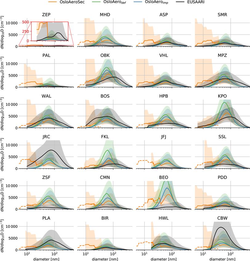
3338         S. M. Blichner et al.: Implementing a sectional scheme for early aerosol growth from new particle formation

       thus does not take into account dynamics within the sub-    aerosol models is that the aerosol mass is divided into “back-
       23.6 nm range (e.g. competition for condensing vapours      ground” tracers and “process” tracers. The background trac-
       and growth of particles over more than one time step).      ers form log-normal modes which decide the number concen-
                                                                   tration, while the process tracers alter this initial log-normal
    2. Including a sectional scheme for this size range brings
                                                                   distribution and their chemical composition. Examples of
       the modelling of early growth closer to first princi-
                                                                   background tracers are dust, sea salt and particles from NPF,
       ples while keeping an acceptable computational cost be-
                                                                   while examples of process tracers are sulfate condensate, sul-
       cause the number of species involved is low. A sectional
                                                                   fate coagulate and organic condensate. After the process trac-
       scheme within this range represents a good alternative
                                                                   ers are applied, the resulting distribution of the “mixtures” is
       to a nucleation mode, which is known to have problems
                                                                   not (necessarily) log-normal anymore. The mass of the trac-
       with transferring particles to the larger mode due to the
                                                                   ers is tracked, and the size distributions for cloud activation
       addition of new particles reducing the median diameter
                                                                   and optical properties are calculated using a look-up table
       of the mode.
                                                                   approach (Kirkevåg et al., 2018).
   In the following we start by describing the aerosol scheme
in NorESM (Sect. 2.1) and then the newly implemented sec-          2.1.1   Chemistry
tional scheme for early growth (Sect. 2.2). Next, in Sect. 4.1,
we show that the new scheme leads to improvements in the           CAM6-Nor has a simplified chemistry scheme for sulfur and
CCN-relevant particle number concentration and size distri-        organic species using the chemical pre-processor MOZART
bution when compared to observational data from Asmi et al.        (Emmons et al., 2010). Pre-calculated monthly mean oxidant
(2011a) consisting of 24 stations in Europe and compiled as        fields consisting of OH, O3 , NO3 and HO2 are read from a
part of the EUSAAR project. Finally, we present the global         file (for discussion see Karset et al., 2018).
changes in the state of aerosols and following cloud proper-          Condensing tracers in the model are H2 SO4 and two
ties in the model with the new scheme (OsloAeroSec) com-           tracers of organics produced by the oxidation of BVOCs,
pared to the original model (Sect. 4.2).                           low-volatility organics (SOAGLV ) and semi-volatile organ-
                                                                   ics (SOAGSV ). The model treats both organic tracers as non-
                                                                   volatile during condensation but represents the volatility by
2     Model description
                                                                   separating which processes each tracer can contribute to:
We start by briefly describing the Norwegian Earth System          SOAGLV can contribute to new particle formation (NPF) and
Model (NorESM) in general before giving a detailed descrip-        early growth, while SOAGSV only contributes to condensa-
tion of its default aerosol model, OsloAero, in Sect. 2.1. Af-     tional growth.
ter this, in Sect. 2.2, we will describe what changes to said         H2 SO4 is emitted directly or produced from oxidation of
aerosol scheme have been introduced in OsloAeroSec. In             SO2 by OH or aqueous-phase oxidation by H2 O2 and O3
general, the aerosol scheme after NPF and early growth is          (Tie et al., 2001). SO2 is either emitted directly or produced
left as it is. The only exception to this is that we have also     by oxidation of dimethyl sulfate (DMS). The condensing or-
included some changes to the diurnal variability of OH, as         ganic tracers, SOAGLV and SOAGSV , are formed from ox-
described in Sect. 2.3.                                            idation isoprene and monoterpenes. The emissions of iso-
   The Norwegian Earth System Model version 2                      prene and monoterpene are calculated online in each time
(NorESM2) (Seland et al., 2020b; Bentsen et al., 2013;             step using the Model of Emissions of Gases and Aerosols
Kirkevåg et al., 2013; Iversen et al., 2013) is largely based      from Nature version 2.1 (MEGAN2.1) (Guenther et al.,
on the Community Earth System Model (CESM) version 2               2012), which is incorporated into CLM5. The atmospheric
(Danabasoglu et al., 2020; Neale et al., 2012). The aerosol        tracer includes only one tracer for monoterpenes, and thus the
scheme in CESM2 is replaced by OsloAero6 (described                emissions of 21 monoterpene species from MEGAN2.1 are
below) (Kirkevåg et al., 2018), and the atmospheric com-           lumped together (Kirkevåg et al., 2018). In addition, produc-
ponent is thus named CAM6-Nor. Furthermore, the ocean              tion of methanesulfonic acid (MSA) by oxidation of DMS
model in CESM2 is replaced by the Bergen Layered Ocean             is taken into account, but since the model lacks a tracer for
Model (BLOM) (Seland et al., 2020b), though this is not            MSA, 20 % of the MSA is put in the SOAGLV tracer and
used in this study as all simulations are run with prescribed      80 % in the SOAGSV .
sea surface temperature (SST) and sea ice concentrations.             For a complete overview of reactions and reaction rates,
The land model is, as in CESM2, is the Community Land              see Table 2 in Karset et al. (2018).
Model (CLM) version 5 (Lawrence et al., 2019).
                                                                   2.1.2   Condensation
2.1    OsloAero: aerosol scheme in NorESM
                                                                   The following is a description of the condensation routine
The aerosol scheme in NorESM, OsloAero, is a production-           in chronological order within one time step. The production
tagged aerosol model. The most notable difference to other         rate, Pgas , of a condensing gas is calculated in the gas-phase

Geosci. Model Dev., 14, 3335–3359, 2021                                            https://doi.org/10.5194/gmd-14-3335-2021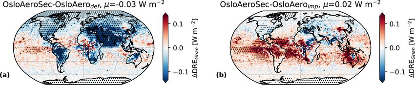
S. M. Blichner et al.: Implementing a sectional scheme for early aerosol growth from new particle formation                 3339

chemistry (Sect. 2.1.1), and the condensation sink, Lcond         where Jnuc [1 s−1 ] is the nucleation rate, A1 = 6.1×10⁻⁷ s−1
[1 s−1 ], is calculated based on the surface area of the back-    and A2 = 3.9×10⁻⁸ s−1 . This is the default nucleation equa-
ground aerosols. Finally, using the initial concentration of      tion in OsloAero and is changed in OsloAeroSec – see
the gas, Cold , from the previous time step, an intermediate      Sect. 2.2.1.
concentration, Cint , is derived by solving the discrete Euler       The survival of particles from nucleation at dnuc ≈ 2 nm,
backwards equation:                                               to the background mode holding the NPF particles with num-
                                                                  ber median diameter 23.6 nm, is parameterized by Lehtinen
Cint − Cold                                                       et al. (2007). The formation rate, Jdmode , of particles at the
             = Pgas − Lcond Cint ,                         (1)
     1t                                                           smallest mode is calculated by
        Cold + Pgas 1t
Cint =                 .                                   (2)
                                                                                               CoagS(dnuc )

        1 + Lcond 1t                                              Jdmode = Jnuc exp −γ dnuc                    ,              (8)
                                                                                                    GR
This intermediate concentration is then used in the forma-
tion of new particles (described in the next section). The NPF    where dnuc is the diameter of the nucleated particle,
subroutine returns an intermediate nucleated mass loss rate,      CoagS(dnuc ) is the coagulation sink of the particles [h−1 ],
Jm,nuc . This nucleated mass is then used to calculate a nucle-   GR is the growth rate [nm h−1 ] of the particle (from H2 SO4
ation loss rate, Lnuc [1 s−1 ].                                   and ELVOC, calculated using Eq. 21 from Kerminen and
                                                                  Kulmala, 2002), and γ is a function of dmode and dnuc :
         Jm,nuc
Lnuc =                                                     (3)
                                                                             "                   #
                                                                                 dmode (m+1)

          Cint                                                           1
                                                                  γ=                          − 1 , m = −1.6.               (9)
                                                                      m+1         dnuc
The new gas concentration, Cnew , is calculated by solving the
discrete Euler backwards equation again, including the loss       Furthermore, CoagS(dnuc ) is calculated from CoagS(dmode )
rate to nucleation.                                               assuming a power-law dependency on diameter,
             Cold + Pgas 1t                                       CoagS(dnuc ) = CoagS(dmode ) · ( ddmode
                                                                                                     nuc m
                                                                                                          ) (Lehtinen et al.,
Cnew =                                                     (4)    2007, Eq. 5).
         1 + Lcond 1t + Lnuc 1t
                                                                     Since Kirkevåg et al. (2018), we have developed an im-
Finally, the total gas lost to condensation and nucleation,       provement to the new particle formation rate (also used
1C, is calculated as follows.                                     in Sporre et al., 2019, 2020). The CoagS(dnuc ) previously
                                                                  included only coagulation onto accumulation- and coarse-
Cnew − Cold = Pgas 1t − 1C                                 (5)    mode particles, but we amended this to include coagula-
1C = Pgas 1t + Cold − Cnew                                 (6)    tion onto all pre-existing particles. This modification gives
                                                                  a lower and more realistic survival rate of particles from for-
   This condensate and/or nucleate, 1C, is then transferred       mation at 2 to 23.6 nm.
to the corresponding process tracer for condensate of the
species (e.g. sulfur condensate) and the background tracer        2.1.4    Coagulation
for new particle formation particles. The mass transfer is
done based on their relative contribution to the total loss       OsloAero takes into account coagulation between Aitken-
rate – i.e. the fraction that is moved to the NPF tracer is       mode and accumulation-mode particles and between Aitken-
fnuc = Lnuc /(Lnuc + Lcond ) and the fraction to condensation     mode and coarse-mode particles, with coagulation co-
is fcond = 1 − fnuc .                                             efficients from the Fuchs form for Brownian diffusion
                                                                  (Sect. 12.3 in Seinfeld and Pandis, 1998). Technically, a nor-
2.1.3    New particle formation                                   malized coagulation sink is calculated for each relevant com-
                                                                  bination of background modes, assuming some fixed prior
The tracers contributing to NPF are H2 SO4 and organics           growth by condensation and/or coagulation. To compute the
(see Makkonen et al., 2014). As mentioned above, SOAGSV           normalized coagulation sink, the size distribution is split into
does not contribute to new particle formation. In addition,       44 bins for the coagulation receiver mode (the larger parti-
only half of the SOAGLV concentration in each time step is        cle), and a coagulation sink with each bin is calculated and
assumed to be low-volatility enough to contribute, and this       normalized by the number concentration. This way, the nor-
fraction will be denoted as ELVOC in the following. The nu-       malized coagulation sink only has to be computed once. In
cleation rate is parameterized with Vehkamäki et al. (2002)       addition, coagulation of aerosols with cloud droplets is esti-
for binary sulfuric acid–water nucleation in the entire atmo-     mated. See Seland et al. (2008) for more details.
sphere, and, in addition, Eq. (18) from Paasonen et al. (2010)
is added to represent boundary layer nucleation. The Paaso-       2.2     OsloAeroSec: new sectional scheme
nen et al. (2010, Eq. 18) parameterization is as follows:
                                                                  The purpose of introducing the sectional scheme is to get
Jnuc = A1 [H2 SO4 ] + A2 [ELVOC],                          (7)    a more realistic growth and loss dynamic within the small-

https://doi.org/10.5194/gmd-14-3335-2021                                            Geosci. Model Dev., 14, 3335–3359, 2021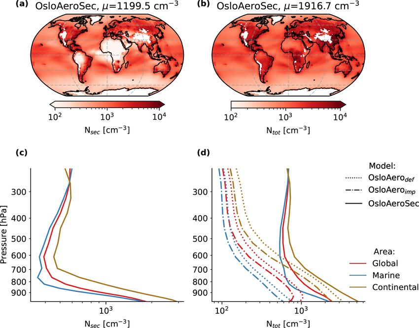
3340           S. M. Blichner et al.: Implementing a sectional scheme for early aerosol growth from new particle formation

est aerosol sizes, with the aim of better modelling aerosol–                  The update was done due to the Riccobono et al. (2014)
climate effects. These smallest particles have insignificant               parameterization being based on more recent research and
effects on climate directly, but rather play a role through                due to the fact that NPF was too high and lasted too long
how they affect the size distribution of the larger particles.             compared to observations with the Paasonen et al. (2010) pa-
For this reason, we do not let the aerosols in the sectional               rameterization in CAM6-NOR. Note that even though it is
scheme directly affect the radiation and cloud parameteriza-               likely that the Riccobono et al. (2014) parameterization rep-
tions, but rather consider only how new particle formation                 resents an improvement compared to Paasonen et al. (2010),
through nucleation, condensation and coagulation affects the               large uncertainties remain due to the fact that the Riccobono
larger aerosols in the modal scheme.                                       et al. (2014) parameterization was developed based on an
   The sectional scheme currently consists of five bins                    ELVOC precursor (pinanediol), rather than actual ELVOC
(though this is flexible), and the bin sizes are set accord-               measurements, and that it does not take into account other
ing to a discrete geometric distribution – the volume-ratio                factors that have been shown to be of importance, like
distribution (Jacobson, 2005, Sect. 13.3) – as follows: let                temperature and ammonia (see e.g. Semeniuk and Dastoor,
d1 , d2 , . . ., d5 be the diameter for each bin and v1 , v2 , . . ., v5   2018).
be the volume per particle for each bin. Each particle in the                 The rate at which particles are introduced into the smallest
bin is assumed to have this same volume (Jacobson, 2005).                  bin, Jdmin , is still parameterized with Eq. (8) defined above
The volume-ratio distribution ensures that the volume per                  (Lehtinen et al., 2007), but with dform = dmin so that the cut-
particle ratio between adjacent bins is fixed; i.e.                        off size is smaller than before.
        vi+1
rv =                                                               (10)    2.2.2    Condensation
         vi
                                                                           The condensation is done in the same way as for OsloAero6,
is fixed. This means that the ratio between the diameter in
                                                                           except that the calculated loss rate to condensation Lcond
adjacent bins, rd , will be
                                                                           is now the sum of loss to condensation onto the back-
        di+1                                                               ground modes from OsloAero and the condensation onto
rd =         = (rv )1/3 .                                          (11)
         di                                                                the sectional bins, Lcond = Lcond,modes +Lcond,sec , in Eqs. (2)
                                                                           and (4). Furthermore, the total gas lost, 1C, calculated by
   Particles are moved into the original aerosol scheme in                 Eq. (6), is then distributed as follows.
the NPF background mode when they reach dmax = 39.6 nm,
which is the volume median diameter of this mode. The vol-                                           Lnuc
                                                                           fnuc =                                                      (14)
ume median diameter is chosen to preserve both number and                           Lnuc + Lcond,modes + Lcond,sec
mass of the particles. Note that dmax is the diameter at which                                    Lcond,sec
the particles are moved to the modal scheme. The choice of                 fcond,sec =                                                 (15)
                                                                                       Lnuc + Lcond,modes + Lcond,sec
dmin , the smallest diameter bin, is flexible, and we have cho-                                    Lcond,modes
sen 5 nm here. So for number of bins, N ,                                  fcond,modes =                                               (16)
                                                                                          Lnuc + Lcond,modes + Lcond,sec
                  1
            dmax    N                                                      Here, fnuc + fcond,sec + fcond,modes = 1. In other words, the
rd =                    ,                                          (12)    condensate added to the modes is Clost,tot · fcond,modes . In the
            dmin
                                                                           same fashion, condensing mass to the sectional scheme is
where dmax = 39.6 nm, dmin = 5 nm and N = 5.                               distributed to the different bins by the strength of their re-
   The sectional scheme includes condensation from two pre-                spective condensational sinks,
cursors, H2 SO4 and SOAGLV , while SOAGSV is considered
                                                                                                     Lcond,bin(di )
to not have low enough volatility to contribute. This gives a              fbin(di ) = fcond,sec ·                  ,                  (17)
total of N (number of bins) ×2 tracers for the model to keep                                          Lcond,sec
track of, keeping computational costs reasonable.                          so that the condensate added to any bin, di , is equal to 1C ·
                                                                           fcond,bin(di ) .
2.2.1       Nucleation                                                         Finally, the condensational growth of particles within the
                                                                           sectional scheme is done in a quasi-stationary structure (Ja-
Nucleation is still parameterized with Vehkamäki et al.
                                                                           cobson, 1997), meaning the particles grow in volume but are
(2002) for binary sulfuric acid–water nucleation in the en-
                                                                           fitted back onto the full stationary grid between each time
tire atmosphere, and the boundary layer nucleation has been
                                                                           step (Jacobson, 2005, Sect. 13.3). This is done by assuming
updated from Paasonen et al. (2010, Eq. 18) (see Eq. 7) to
                                                                           that (1) the total volume is constant before and after the trans-
Riccobono et al. (2014):
                                                                           fer between the bins, and (2) the total number is the same. Let
Jnuc = A3 [H2 SO4 ]2 [ELVOC]                                       (13)    vi and vi+1 be the volume of a particle in bin i and the next
                                                                           bin, i + 1, prior to any growth. Let vi0 be the volume of a par-
where A3 = 3.27 × 10⁻²¹ cm6 s−1 .                                          ticle in bin i after growth. Furthermore, let Ni be the number

Geosci. Model Dev., 14, 3335–3359, 2021                                                       https://doi.org/10.5194/gmd-14-3335-2021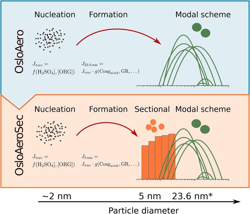
S. M. Blichner et al.: Implementing a sectional scheme for early aerosol growth from new particle formation                 3341

of particles in bin i prior to growth and 1Ni+1 be the num-         based on whether it is before or after sunrise. Since OH in
ber of particles moved to the next bin i + 1. Since we do not       particular is very important for the diurnal cycle of H2 SO4 ,
have any evaporating species, we can easily solve the equa-         this leads to more or less a step function in H2 SO4 concen-
tion conserving both the number and volume of aerosol for           trations as well, which is not very realistic in terms of NPF.
each species:                                                       We therefore implemented a simple sine shape to the daily
                                                                    variation in place of the step function.
vi0 Ni = vi (Ni − 1Ni+1 ) + vi+1 1Ni+1 ,                    (18)

and solving for 1Ni+1 gives                                         3     Model simulations and output post-processing
                 vi0
                   − vi
1Ni+1 = Ni ·              .                                 (19)    3.1    Simulation description
                vi+1 − vi
   After the particle mass is moved in this way, the freshly        In the following analysis we include simulations with three
nucleated particles from the same time step are added to the        versions of the CAM6-Nor.
smallest bin. The rationale behind this is that the nucleated
                                                                        – A simulation with OsloAeroSec, referred to simply as
particles in the same time step do not take part in the conden-
                                                                          “OsloAeroSec” (see Sect. 2.2)
sation sink calculation, and thus including them before the
redistribution of mass on the sectional grid would only imply           – A simulation with the default version of OsloAero (see
adding particles with no added condensate.                                Sect.2.1), referred to as “OsloAerodef ”
   The time step within the nucleation and condensation code
is locally divided in two compared to the rest of the code              – A simulation with the default version of OsloAero, but
(thus 15 min), and if the particles in the sectional scheme               with the same changes to the nucleation rate (Eq. 13)
grow fast enough to skip a bin, the time step is further di-              and oxidants (see Sect. 2.3) as OsloAeroSec, referred to
vided in two until it is small enough.                                    as “OsloAeroimp ”

2.2.3    Coagulation                                                The last simulation, OsloAeroimp , is added in order to sep-
                                                                    arate the changes made in OsloAeroSec to the nucleation
In addition to the unchanged coagulation in the original            rate and the diurnal concentration in the oxidants (described
OsloAero scheme (see Sect. 2.1.4), we calculate the coag-           above) from the effect of adding a sectional scheme. The sim-
ulation sink of the sectional particles onto all larger parti-      ulation characteristics are also summarized in Table 1.
cles. This is done in the same way between particles in the            NorESM2 is run with CAM6-Nor (release-noresm2.0.1,
original OsloAero scheme, in that a normalized coagulation          https://github.com/NorESMhub/NorESM,            last  access:
sink is calculated for each background mode by dividing the         28 May 2021; Kirkevåg et al., 2018) coupled to the Com-
size distribution into 44 bins. When sectional particles co-        munity Land Model version 5 (CLM5) (Lawrence et al.,
agulate with particles in the “modal” scheme, their mass is         2019) in BGC (biogeochemistry) mode and prognostic
transferred to the corresponding process tracer for conden-         crops. We use a 1.9◦ (latitude) × 2.5◦ (longitude) resolution
sate. This is done for simplicity and because the alternative       grid with 32 height levels from the surface to ∼ 2.2 hPa in
would be to place them in the coagulation tracers – one of          hybrid sigma coordinates. We use prescribed sea surface
the process tracers – in the original scheme, which will only       temperature (SST) and sea ice concentrations at 1.9 × 2.5◦
contribute to changes in the larger particles.                      resolution (Hurrell et al., 2008). Simulations are run from
   In addition to this, coagulation between the particles in the    2007 to and throughout 2014 with CMIP6 historical emis-
sectional scheme is taken into account. When two particles          sions and greenhouse gas concentrations (Seland et al.,
in the sectional scheme collide, this results in the loss of the    2020b) as well as nudged meteorology (horizontal wind and
particle in the smaller bin and the addition of mass to the         surface pressure) to ERA-Interim (ECMWF, 2011) using a
particle in the larger bin. After this is done in each time step,   relaxation time of 6 h (Kooperman et al., 2012) (as described
the mass in the sectional scheme is redistributed in the same       in Karset, 2020, Sect. 4.1). The year 2007 is discarded as
way as after condensation (see previous section).                   spin-up. The initial conditions for all simulations are taken
                                                                    from a simulation with CAM6-Nor run from 2000 and
2.3     Chemistry: changes to oxidant diurnal variation             throughout 2006.

The oxidant concentrations of the hydroxyl radical (OH), ni-        3.2    Post-processing of model output
trate radical (NO3 ), hydroperoxy radical (HO2 ) and ozone
(O3 ) in the model are prescribed by 3D monthly mean fields         All figures, except comparisons to observations (described
(see Seland et al., 2020b). On top of this, a diurnal cycle is      below), are produced from monthly mean output files from
applied to OH, HO2 and NO3 . In the default version of the          the model. When we present figures showing averaged values
model, the diurnal cycle for OH is basically a step function        over maps, these are either column burdens or “near-surface”

https://doi.org/10.5194/gmd-14-3335-2021                                               Geosci. Model Dev., 14, 3335–3359, 2021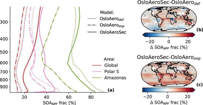
3342         S. M. Blichner et al.: Implementing a sectional scheme for early aerosol growth from new particle formation

Table 1. Simulation overview. See the detailed description in Sect. 3.

          Simulation           Nucleation parameterization             Oxidant treatment                     Early growth treatment
          OsloAeroSec          A3 [H2 SO4 ]2 × [ELVOC]a                Improved diurnal variation            Lehtinen et al. (2007) + sectional scheme
          OsloAeroimp          A3 [H2 SO4 ]2 × [ELVOC]a                Improved diurnal variation            Lehtinen et al. (2007)
          OsloAerodef          A1 [H2 SO4 ] + A2 [ELVOC]b              Default diurnal variation             Lehtinen et al. (2007)

        A1 = 6.1 × 10⁻⁷ s−1 . A2 = 3.9 × 10⁻⁸ s−1 . A3 = 3.27 × 10⁻²¹ cm6 s−1 . a Riccobono et al. (2014). b Paasonen et al. (2010).

Table 2. Region overview. These regions are used to create vertical average profiles.

                                   Region name          Description                              Latitude           Longitude
                                   Continental          Grid boxes with > 50 % land
                                   Marine               Grid boxes with < 50 % land
                                   Global
                                   Polar N                                                       66.5–90◦ N         180◦ W–180◦ E
                                   Polar S                                                       66.5–90◦ S         180◦ W–180◦ E
                                   Amazonas                                                      16◦ S–2◦ N         74–50◦ W

averages of the variable in question. The near-surface av-                               tains time series of hourly data for number concentrations
erages are calculated as the average of all grid cells below                             of particles with diameters between 30 and 50 nm (N30–50 ),
850 hPa, weighted by the grid cell pressure thickness to ac-                             50 and 500 nm (N50–500 ), 100 and 500 nm (N100–500 ), and
count for the mass in the grid cell. Cloud radiative effects and                         finally 250 and 500 nm (N250–500 ). In this study, we focus
direct radiative effects are calculated as described in Ghan                             on the concentration of particles with diameters between 50
(2013).                                                                                  and 100 nm, i.e. N50–100 = N50–500 − N100–500 . Throughout
   For the model-to-model comparisons, we include an anal-                               the simulation period, we output hourly mean values describ-
ysis of whether the change is significant. Dots are included                             ing the modelled size distribution.
in the plots to indicate where the difference between the two                               The model outputs a log-normal fitting to the size distri-
models is significant with a two-tailed paired Student’s t test                          bution in terms of parameters for 12 log-normal modes. In
with a 95 % confidence interval.                                                         other words, the total size distribution is
   When we compare the model runs, we compare the model
                                                                                                  12
version with and without an explicit treatment of the smallest                            dN      X   dNi
                                                                                                =           .                                             (20)
particles. We therefore introduce the following subgroups of                             d(dp )    i
                                                                                                     d(dp )
particle number concentration. We refer to particle number
concentrations excluding particles in the sectional scheme as                                        dNi
                                                                                         Each term d(d p)
                                                                                                          is furthermore defined in terms of output pa-
Na . This includes all the particles for the OsloAero simula-                            rameters from the modal number median diameter, dm,i , ge-
tions (OsloAerodef and OsloAeroimp ) but excludes the parti-                             ometric standard deviation, Si , and the number concentration
cles still in the sectional scheme for OsloAeroSec. Further-                             in the mode, Ni :
more, the total number of aerosols we refer to as Ntot , and the                                                                                  !
concentration of aerosols in the sectional scheme will be re-                             dNi           Ni           (log(dp ) − log(dm,i ))2
                                                                                                =            √ exp −                                  .   (21)
ferred to as Nsec . Finally, the aerosol scheme also tracks the                          d(dp )   dp log(Si ) 2π            2 log(Si )
number of particles in the modal scheme originating from
NPF, and this we denote as NNPF . This is summed up in Ta-                                  For each mode, we can then calculate the number of parti-
ble 3. Note that changes in NNPF and Na in general follow                                cles in a size range from diameter d1 to d2 by
the same patterns because we do not introduce changes to                                 Ni,d1 −d2 = Ni (d < d2 ) − Ni (d < d1 ),                         (22)
particles other than those from NPF.
                                                                                         where Ni is the cumulative distribution function of the distri-
3.3    Processing of model output data prior to                                          bution in Eq. (21), and thus
       comparison with observations                                                                    1 1

                                                                                                                   log(x) − log(dm,i )

                                                                                         Ni (d < x) = + erf            √                 .         (23)
                                                                                                       2 2              2 log(Si )
We compare the nudged model simulations for the years
2008 and 2009 to observed size distributions from the EU-                                The total P
                                                                                                   number concentration in a size range is thus
SAAR dataset from Asmi et al. (2011a). The dataset con-                                  Nd1 −d2 = 12i=1 Ni,d1 −d2 . We calculate these variables for

Geosci. Model Dev., 14, 3335–3359, 2021                                                                         https://doi.org/10.5194/gmd-14-3335-2021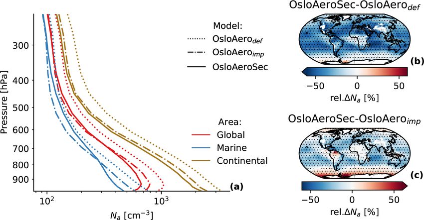
S. M. Blichner et al.: Implementing a sectional scheme for early aerosol growth from new particle formation                   3343

Table 3. Model variable definitions.

                         Variable name   Definition
                         Na              Number of particles excluding those in the sectional scheme
                         Ntot            Number of particles including those in the sectional scheme
                         Nsec            Number of particles in the sectional scheme
                         NNPF            Number of particles from NPF excluding those in the sectional scheme
                         Nd1 −d2         Number of particles with diameter d such that d1 ≤ d ≤ d2
                         Nd1             Number of particles with diameter d such that d1 ≤ d

each hour and compute further statistics from the result. By         BEO). The exceptions that stand out are e.g. CBW, JRC,
using such a fine time resolution, we avoid a common impre-          ZEP and KPO, where all versions of the model do rather
cision arising when averaging the parameters of the size dis-        poorly in both absolute numbers and in terms of represent-
tribution, rm,i and Si , over a longer time period (i.e. monthly     ing the annual variability. This might indicate that aerosol or
output).                                                             precursor emissions in the model are not accurate e.g. due
   Furthermore, for the comparison of size distributions, we         to local sources that are unaccounted for in the model. For
              dN           dN
calculate d log(dp)
                    = dp d(d p)
                                 for an array of diameters and       CBW, NPF should not be an important source of aerosols
compute further statistics from the hourly values.                   during winter and autumn (Mamali et al., 2018), so it is
                                                                     likely that other aerosols are responsible for the underesti-
                                                                     mation during these seasons. Dall’Osto et al. (2018) note
4     Results and discussion                                         a strong influence of local anthropogenic emissions at this
                                                                     station, which is likely not captured in the CMIP6 emis-
4.1    Comparison to EUSAAR dataset                                  sions. However, during summer, the model may well show
                                                                     an underestimation of production of particles from NPF,
In this comparison we focus on N50–100 because particles             which becomes slightly worse with OsloAeroSec. Accord-
smaller than 50 nm are unlikely to be relevant for CCN and           ing to Dall’Osto et al. (2018), NPF should be most frequent
particles above 100 nm are less effected by the changes to the       in JRC and KPO during spring, which the N50–100 does
NPF scheme (see e.g. the size distributions in Fig. 4).              not really reflect, probably due to other particles dominat-
   Figures 2 and S4 in the Supplement show the distribution          ing the annual variability. Furthermore, at ZEP station, the
of the modelled minus the observed values for N50–100 at             concentrations are underestimated in all months except late
hourly resolution and with all valid station data included.          autumn and winter. At this station the concentrations in the
   From Fig. 2 we can see a clear improvement with                   sectional scheme (see Figs. 4 and S12–S15 in the Supple-
OsloAeroSec compared to both OsloAerodef and                         ment) reveal that there are relatively many particles forming
OsloAeroimp . The improvement is most pronounced in                  at this location, but they do not survive to 50 nm. All mod-
summer, when OsloAerodef and OsloAeroimp overestimate                els perform badly here, with OsloAeroSec and OsloAeroimp
N50–100 , while it is also clear in autumn and spring. It is         performing slightly worse than OsloAerodef . In PLA and
also encouraging that OsloAeroSec has a clear decrease in            WAL, the OsloAeroSec results in values that are too low,
the times when the number concentration is highly overes-            while OsloAerodef and OsloAeroimp perform better. In sta-
timated, while there is not a similar increase in times when         tion MHD, FKL, ZSF, CMN and BEO, the model overes-
it is underestimated. Furthermore, we see that changes to            timation of N50–100 is reduced in OsloAeroSec but is still
nucleation parameterization and diurnal variation in oxidants        significantly too high.
in OsloAeroimp reduce the bias compared to OsloAerodef .                The normalized root mean square error (NRMSE) is im-
In winter, NPF is low, so we see little difference between           proved with OsloAeroSec for both N50–100 and N50–500 ,
the different schemes. Figure S4 shows the same as Fig. 2            while it stays more or less the same for N100–500 . The
but for each individual station. OsloAeroSec (OsloAeroSec)           NRMSE is shown in Fig. S5 in the Supplement and is cal-
shows improvement against OsloAero (OsloAerodef and                  culated for each season and each model version using hourly
OsloAeroimp ) in most stations during JJA, while sometimes           resolution and all available data. The greatest improvement is
underestimating N50–100 in MAM (e.g. VHL, MPZ, HWL).                 seen in N50–100 and in summer, followed by SON and MAM,
   The annual variability of both models and observations            while DJF is mostly unchanged. N50–500 shows improvement
is shown in Fig. 3, where the monthly median (solid line)            in the same seasons, while there only small improvements in
and percentiles (16th to 84th) are plotted for each station.         prediction skill for N100–500 . The lack of change in predic-
Again it is clear that OsloAeroSec in general reduces the            tion skill for particles larger than 100 nm likely originates
high bias of OsloAerodef and OsloAeroimp , especially when           from the fact that in CAM6-Oslo, the NPF particles no not
the bias is very high (e.g. OBK, HPB, FKL, ZSF, CMN,

https://doi.org/10.5194/gmd-14-3335-2021                                               Geosci. Model Dev., 14, 3335–3359, 2021
3344 S. M. Blichner et al.: Implementing a sectional scheme for early aerosol growth from new particle formation
Figure 2. Seasonal distribution of modelled N50–100 minus observed N50–100 for all EUSAAR stations (Asmi et al., 2011a). We use hourly
resolution, and all available station data are included.
change mode by condensational growth – rather, the whole Aitken-mode particles, this is likely due to other aerosol
mode grows in number median diameter. Thus, the variabil- sources not being adequately represented in the model. This
ity in concentrations of particles larger than 100 nm is dom- leads to an underestimation of coagulation sink and hence an
inated by primary particle emissions, which we do not alter overestimation of the formation rate. To the same effect, the
here. condensation sink may be too low, again leading to too many
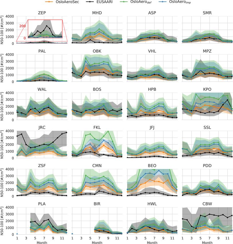
Even though the N50–100 improves, Fig. 4 reveals that the new particles forming. This is particularly clear in the Arc-
concentrations at smaller sizes are overestimated in most lo- tic station Zeppelin (ZEP), where the measurements show a
cations. The figure shows the size distribution of particles at peak in particles between 100 and 200 nm, which are com-
each station from both observations and the three versions pletely missing in the models. The combination of an overly
of CAM6-Nor. For the sectional scheme, the distribution is high formation rate and a slow condensation growth rate
the sum of particles in the sectional scheme and the modal leads to too many particles in the smaller sizes.
scheme. This is why it has “spikes” and why there is often Overall, adding the explicit treatment of the smaller parti-
a large reduction in dN/dlog10 D at the intersection between cles in OsloAeroSec does improve the representation of CCN
the sectional scheme and the modal scheme, which might be relevant particles in the model. We especially get a reduction
misunderstood to mean that disproportionately many parti- in number concentrations of diameters above 50 nm at which
cles are lost in the transition between the sectional and modal they are significantly overestimated.
scheme. The distribution in the sectional scheme, without
adding the modal particles, is shown by the dashed line. One 4.2 Comparison to original model
important reason why the sectional scheme overestimated the
number of the particles at the smallest sizes may be that the The following section will present general differences in
number of particles above ∼ 100 nm is underestimated in all OsloAeroSec compared to the two versions of the original
the model versions in most of the stations (see e.g. the dis- model, OsloAerodef and OsloAeroimp . For this analysis, we
tribution of particle surface areas in Fig. S11 in the Supple- make use of the full global model output in monthly mean
ment). resolution. We will start by comparing the particle number
This is particularly pronounced in summer, when the num- concentrations and properties of the aerosols. The original
ber of particles in the sectional scheme is particularly high version of the CAM6-Nor aerosol scheme does not explicitly
(see Fig. S13). Since NPF mostly influences nucleation and model the smallest particles, so in order to get an apples-
to-apples comparison, we focus on properties relevant for
Geosci. Model Dev., 14, 3335–3359, 2021 https://doi.org/10.5194/gmd-14-3335-2021S. M. Blichner et al.: Implementing a sectional scheme for early aerosol growth from new particle formation 3345
Figure 3. N50–100 monthly median (solid line) and percentiles (shaded, 16th to 84th) for each station for each model version and the
observed values (Asmi et al., 2011a). Stations where the full graph is not shown due to the axis limits are shown in full in Fig. S6 in
the Supplement. Zeppelin (ZEP), Mace Head (MHD), Aspvreten (ASP), SMEAR II (SMR), Pallas (PAL), Kosetice (OBK), Vavihill (VHL),
Melpitz (MPZ), Waldhof (WAL), Bösel (BOS), Hohenpeissenberg (HPB), K-Puszta (KPO), JRC-Ispra (JRC), Finokalia (FKL), Jungfraujoch
(JFJ), Schauinsland (SSL), Zugspitze (ZSF), Monte Cimone (CMN), BEO Moussala (BEO), Puy de Dôme (PDD) Preila (PLA), Birkenes
(BIR), Harwell (HWL), Cabauw (CBW).
climate, as represented by the modal aerosol scheme when 4.2.1 Aerosols
comparing OsloAeroSec to OsloAerodef and OsloAeroimp .
See Table 3 for a summary of the definitions of the variables The total number of particles, Ntot , increases in OsloAeroSec
defining number concentration. We then proceed to changes compared to OsloAerodef and OsloAeroimp due to the addi-
in cloud properties and finally the radiative effect. tion of particles not explicitly treated before. In Fig. 5 the
absolute number of sectional particles, Nsec , in OsloAeroSec
is shown (a and c) together with the total number of parti-
cles, Ntot (right, b and d). The maps in Fig. 5a and b show
near-surface averages, as defined in Sect. 3.2. As can be
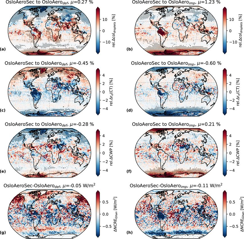
https://doi.org/10.5194/gmd-14-3335-2021 Geosci. Model Dev., 14, 3335–3359, 20213346 S. M. Blichner et al.: Implementing a sectional scheme for early aerosol growth from new particle formation Figure 4. Median (solid line) particle number size distribution and shading from the 16th to 84th percentiles for observations (Asmi et al., 2011a) and models. All data when and where observations are available are included. seen from Fig. 5d, the change is particularly strong in the has fewer particles close to the surface, while the difference upper troposphere, where Ntot is very low in OsloAeroimp is reduced further up in the atmosphere. In the free tropo- and OsloAerodef because the smallest particles are simply not sphere, i.e. further away from the surface, the difference be- represented in these model versions. comes positive and OsloAeroSec lets more particles survive Figure 6a shows averaged profiles of Na for each model through early growth. For the global average this happens version, while Fig. 6b and c show maps of the near-surface roughly at 700 hPa, while over ocean it happens at 800 hPa. relative difference in OsloAeroSec compared to OsloAerodef Over the continents, OsloAeroimp is always higher, though and OsloAeroimp , respectively. On average, the global near- the difference decreases with height. From these results, we surface Na decreases in OsloAeroSec by 15 % compared to can conclude that on average the sectional scheme produces OsloAeroimp and 36.2 % compared to OsloAerodef . However, more particles in more remote regions both horizontally and at high latitudes the change relative to OsloAeroimp is small, vertically. or positive, especially over the Southern Ocean. When con- In all model versions, the growth of the particles from sidering the vertical change shown in Fig. 6a, OsloAeroSec nucleation to the smallest mode happens by condensa- Geosci. Model Dev., 14, 3335–3359, 2021 https://doi.org/10.5194/gmd-14-3335-2021
S. M. Blichner et al.: Implementing a sectional scheme for early aerosol growth from new particle formation                        3347

Figure 5. Modelled particle number concentrations. Panels (a) and (b) show maps of the near-surface average concentrations for Nsec (a)
and Ntot (b) in OsloAeroSec. Panels (c) and (d) show average profiles globally, over continents (continental) and over ocean (marine) for
Nsec (c) and Ntot (d). In (d), OsloAerodef and OsloAeroimp are also included.

Figure 6. Comparison of Na from OsloAerodef and OsloAeroimp to OsloAeroSec. (a) Profiles of the mean of regions (global, marine and
continental) for the model versions. (b, c) The relative difference in the near-surface mean of OsloAeroSec compared to OsloAerodef and
OsloAeroimp , respectively. Areas where the difference is significant (95 %) are marked with dots.

tion of the two tracers H2 SO4 and SOAGLV . The rela-                  pared to OsloAerodef , and secondly, globally it goes up
tive contribution of H2 SO4 and SOAGLV to this growth                  with OsloAeroSec. We start by exploring the difference
changes with OsloAeroSec but, interestingly, also between              between OsloAerodef and OsloAeroimp . These two simula-
OsloAerodef and OsloAeroimp . Figure 7a shows the sec-                 tions have the same parameterization for survival of parti-
ondary organic aerosol (SOA) fraction of the particles that            cles from nucleation up to the model scheme (see Sect. 2.2),
have survived to the modal scheme averaged over regions.               but OsloAeroimp has an improved diurnal variation in the
Firstly, the SOA fraction goes down in OsloAeroimp com-                oxidants, resulting in a higher diurnal peak in H2 SO4 (not

https://doi.org/10.5194/gmd-14-3335-2021                                                  Geosci. Model Dev., 14, 3335–3359, 2021
3348        S. M. Blichner et al.: Implementing a sectional scheme for early aerosol growth from new particle formation

Figure 7. The SOA fraction of NNPF mass (SOANPF ), i.e. the fraction of the growth of the particles before they reach the modal scheme,
which is due to organics. (a) Profiles for regions (global, polar south, Amazonas) with each model. (b, c) The difference in the near-surface
mean values for OsloAeroSec minus OsloAerodef and OsloAeroimp (c), respectively. Areas where the difference is significant (95 %) are
marked with dots.

shown). Additionally, the nucleation parameterization in                     The strength and sign of the change in number concentra-
OsloAeroimp is of the form H2 SO4 2 × ELVOC, meaning that                tion between OsloAeroSec and the original model vary with
as H2 SO4 increases, the nucleation rate increases to the                location.
power of 2, while in OsloAerodef the increase is linear with                 To investigate what conditions lead to the changes in
both H2 SO4 and ELVOC. Furthermore, because the growth                   NPF particles, we focus on the difference in NNPF between
from the nucleation to modal scheme happens within one                   OsloAeroSec and OsloAeroimp and analyse its relationship
time step in these simulations, the fraction of growth from              to relevant variables in OsloAeroimp . Thus, we can analyse
SOA is entirely based on H2 SO4 and ELVOC at the moment                  under which conditions in the model (polluted, clean, high
of nucleation. This means that if most of the particles form             NPF etc.) NNPF increases or decreases with the sectional
when H2 SO4 is at its highest, H2 SO4 will also dominate the             scheme. Figure 8 shows the relationship for nucleation rate
post-nucleation growth. This explains the reduced contribu-              (Jnuc , a), growth rate (GR, b), H2 SO4 (c), SOAGLV (d), NNPF
tion of SOA in OsloAeroimp relative to OsloAerodef .                     (e) and coagulation sink for newly formed particles (CoagS,
   The change seen in OsloAeroSec compared to                            f). This 2D histogram includes each grid cell below 100 hPa,
OsloAerodef and OsloAeroimp , on the other hand, can                     and monthly mean values are used for each grid cell.
be explained by two factors: (1) though OsloAeroSec has the                  Firstly, most of the variables show a branch with a strong
same changes to oxidants and nucleation parameterization as              negative relationship with the change in NNPF (1NNPF ). Fur-
OsloAeroimp , the particles grow in the sectional scheme over            ther investigation shows that the grid cells that constitute
more than one time step and are thus exposed to different                this branch are mainly close to the surface and, as can be
concentrations of H2 SO4 and SOAGLV . Thus, the concentra-               seen from Fig. 8e, where NNPF and CoagS are high. In other
tions at the time of nucleation will be less dominant for the            words, what we are seeing is that in regions with high CoagS
growth. (2) In OsloAerodef and OsloAeroimp only ELVOC,                   and NNPF , the sectional scheme drastically reduces the num-
which is 50 % of the SOAGLV , will contribute to growing                 ber of particles that survive and reduces it more the higher
the particles up to the modal scheme, while in OsloAeroSec               they were initially in OsloAeroimp . This resembles what we
100 % of the SOAGLV can contribute after the particles have              saw when comparing to station data, with the very high over-
reached the sectional scheme (5 nm), thus increasing the                 estimations particularly reduced.
SOA fraction. The result is a combination of these effects; in               For the other grid cells, in which NNPF and CoagS are
some regions, like over the Amazon, the effect seems to be               lower, there is another branch showing a positive relation-
dominated by the change in nucleation timing such that the               ship with GR, H2 SO4 and SOAGLV . From panels (e) and (f),
SOA fraction goes down compared to OsloAerodef . In most                 it is clear that these grid cells have NNPF concentrations un-
regions the effect is that the SOA fraction increases.                   der roughly 100 cm−3 and CoagS under roughly 10−3 h−1 .
   Note that the changes in hygroscopicity from this are mi-             In this regime the sectional scheme allows more particles to
nor and mitigated by the fact that additional condensate is              survive, and condensational growth is more important.
added to the particles after they reach the modal scheme.

Geosci. Model Dev., 14, 3335–3359, 2021                                                    https://doi.org/10.5194/gmd-14-3335-2021
You can also read