Impact of unplanned service disruptions on urban public transit systems - arXiv
←
→
Page content transcription
If your browser does not render page correctly, please read the page content below
Impact of unplanned service disruptions on urban public transit systems

                                                   Baichuan Moa,∗, Max Y von Franqueb , Haris N. Koutsopoulosc , John Attanuccid , Jinhua Zhaoe
                                                   a
                                                       Department of Civil and Environmental Engineering, Massachusetts Institute of Technology, Cambridge, MA 02139
                                                   b
                                                       Department of Urban Studies and Planning, Biology, Massachusetts Institute of Technology, Cambridge, MA 02139
                                                              c
                                                                Department of Civil and Environmental Engineering, Northeastern University, Boston, MA 02115
                                                                                d
                                                                                  Massachusetts Institute of Technology, Cambridge, MA 20139
                                                          e
                                                            Department of Urban Studies and Planning, Massachusetts Institute of Technology, Cambridge, MA 20139
arXiv:2201.01229v1 [stat.AP] 3 Jan 2022

                                          Abstract

                                                 This paper proposes a general unplanned incident analysis framework for public transit systems from
                                          the supply and demand sides using automated fare collection (AFC) and automated vehicle location (AVL)
                                          data. Specifically, on the supply side, we propose an incident-based network redundancy index to analyze the
                                          network’s ability to provide alternative services under a specific rail disruption. The impacts on operations
                                          are analyzed through the headway changes. On the demand side, the analysis takes place at two levels:
                                          aggregate flows and individual response. We calculate the demand changes of different rail lines, rail
                                          stations, bus routes, and bus stops to better understand the passenger flow redistribution under incidents.
                                          Individual behavior is analyzed using a binary logit model based on inferred passengers’ mode choices and
                                          socio-demographics using AFC data. The public transit system of the Chicago Transit Authority is used as a
                                          case study. Two rail disruption cases are analyzed, one with high network redundancy around the impacted
                                          stations and the other with low. Results show that the service frequency of the incident line was largely
                                          reduced (by around 30%∼70%) during the incident time. Nearby rail lines with substitutional functions were
                                          also slightly affected. Passengers showed different behavioral responses in the two incident scenarios. In the
                                          low redundancy case, most of the passengers chose to use nearby buses to move, either to their destinations
                                          or to the nearby rail lines. In the high redundancy case, most of the passengers transferred directly to nearby
                                          lines. Corresponding policy implications and operating suggestions are discussed.
                                          Keywords: Incident analysis; Rail disruptions; Redundancy index; Smart card data;

                                          1. Introduction

                                                 Urban public transit systems play a crucial role in cities worldwide, transporting people to jobs, homes,
                                          outings, and a variety of other activities. Millions rely on urban transit systems to provide them with
                                          transportation. However, transit systems are susceptible to unplanned delays and service disruptions caused
                                          by equipment, weather, passengers, or other internal and external factors.
                                                 Mitigating the impact of unplanned service disruptions is an important task for urban transit agencies. For
                                          this reason, it is important to recognize how a transit system is affected by service disruptions. The analysis
                                          framework for incident impacts can be summarized in Table 1. The two main dimensions of analysis, supply

                                          ∗
                                              Corresponding author

                                          Preprint submitted to Transportation                                                                            January 5, 2022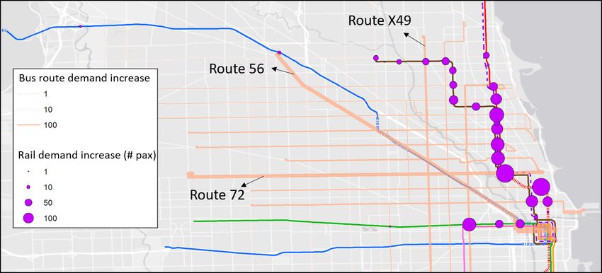
and demand, can further be broken down into “network performance” and “service” for supply analysis and
“passenger flow” and “individual behavior” for demand analysis.

                                    Table 1: Analysis framework for incident impacts

                   Analysis tasks              Description
                   Network performance         Indicators such as resilience, vulnerability, redundancy
        Supply
                   Service                     Changes in agency’s operations (e.g., headway, routing)
                   Passenger flow              Demand changes at different stations, lines
        Demand
                   Individual behavior         Passengers’ mode choices under incidents

    The network performance analysis usually uses graph theory-based techniques to calculate indicators
related to incidents (Berdica, 2002; Xu et al., 2015; Yin et al., 2016; Zhang et al., 2018), such as network
resilience, vulnerability, redundancy, and a variety of other properties. The service analysis focuses on
changes in an agency’s operations during the incident period including headway, routing, staffing, and other
operator-controlled factors designed to mitigate the incidents. From the demand point of view, passenger
flow analysis investigates the demand changes at different stations, lines, or regions of a network, presenting
passenger’s choices and flow redistribution after service disruptions. The individual behavior analysis focuses
on studying the individual’s response (such as mode choices, waiting time tolerance) to the incident and
its relationship to the individual’s characteristics (e.g., travel histories, demographics) (Rahimi et al., 2020,
2019). Surveys are usually used for such studies.
    Previous research has used a variety of methods to analyze the impact of service disruptions. Of these
methods, the three most common are graph theory-based, survey-based, and simulation-based. Graph theory-
based methods usually derive resilience or vulnerability indicators based on the network topology (Yin et al.,
2016; Zhang et al., 2018; Xu et al., 2015; Berdica, 2002). These methods are effective for understanding
high-level network properties related to incidents. Survey-based methods investigate passenger behavior
during and opinions about the incident (Currie and Muir, 2017; Murray-Tuite et al., 2014; Fukasawa et al.,
2012; Teng and Liu, 2015; Lin et al., 2018). Passengers’ individual-level behavior is analyzed and understood
using econometric models. Simulation-based methods simulate passenger flows on the transit network under
incident scenarios (Balakrishna et al., 2008; Suarez et al., 2005; Hong et al., 2018). These studies can
output many metrics of interest such as vehicle load changes, additional travel delays caused by incidents,
distribution of the impact, etc.
    Recently, automated data collection systems in transit networks enable a data-driven analysis of the
impacts of service disruptions. The two major sources are automatic fare collection (AFC) and automatic
vehicle location (AVL) data. AFC data is collected when passengers tap their transit cards on smart card
readers (in buses or rail station gates). The records include times, locations and card IDs. Depending on
whether the fare system requires passengers to tap out, AFC data may only include tap-in records or both
tap-in and tap-out records. AVL data records vehicle’s (bus and train) time-dependent locations based on
GPS and train tracking systems. From the AVL records, information such as headways can be inferred.
Recently, a limited number of studies have been conducted using AFC and AVL data to look at unplanned

                                                           2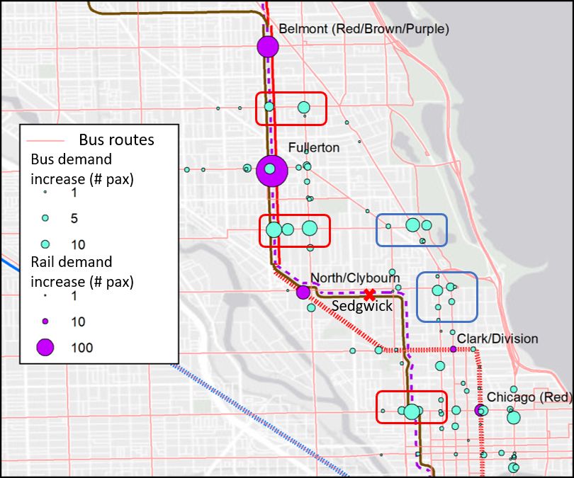
transit disruptions. For example, Sun et al. (2016) analyzed three types of abnormal passenger flows during
unplanned rail disruptions using AFC data with both tap-in and tap-out records. Tian and Zheng (2018)
proposed a classification model to predict whether commuters switch from rail to other transportation modes
because of unexpected travel delays using six months of AFC data.
    However, despite numerous studies on incident analysis, there are still research gaps. First, for the
graph theory-based approaches, the network indicators such as redundancy are usually defined for the whole
network, an OD pair, or a link, and do not consider the influence of the disruption duration. Incidents usually
cause service interruptions at multiple links depending on the power system and rail track configuration.
And the duration of an incident can vary from 5 minutes to several hours, resulting in various impacts on
the network. An incident-based indicator that reflects the network’s redundancy under an actual incident
with a specific location and duration is needed. Second, the studies that leverage AFC data to analyze
passengers’ mode choices under disruptions are very limited. Such approachs would require the inference of
both individual choices and socio-demographic information from the AFC data. Third, most of the previous
studies on incident analysis only addressed one or two aspects in Table 1 using case studies of a single
incident. A comprehensive study that analyzes all four dimensions of the problem with comparable case
studies using AFC and AVL data is missing from the literature.
    The paper aims to fill these research gaps by developing a data-driven methodology for the comprehensive
analysis of the impact of unplanned rail disruptions on passengers and operations. Specifically, on the supply
side, we propose an incident-based network redundancy index to analyze the ability of bus and rail networks to
provide alternative services under a specific rail disruption. The impacts on operations are evaluated through
headway changes across the systems. On the demand side, we calculate the demand changes at different
rail lines, rail stations, bus routes, and bus stops to better understand the passenger flow redistribution under
incidents. Individual behavior is analyzed using a binary logit model based on inferred passengers’ mode
choices and socio-demographics using AFC data. The public transit system of the Chicago Transit Authority
(CTA) is used for a case study with two rail disruptions, one of which has high network redundancy and the
other low.
    The main contributions of this paper are as follows:

    • Propose an incident-based network redundancy index to reflect the system’s ability to provide alterna-
      tive services considering the integrated bus and rail systems. The index leverages the proposed concept
      of path throughput to incorporate the impact of the incident duration on the redundancy calculation.

    • Develop an incident analysis framework using AFC and AVL data and apply it to incidents with
      different characteristics. Specifically, we analyze two types of incidents with high and low redundancy
      separately from both demand and supply perspectives.

    • Propose an individual mode choice analysis method using AFC data. The approach includes a travel
      mode inference model and a passenger demographics extraction model. To the best of our knowledge,
      this is the first study that adopts AFC data for individual mode choice analysis during incidents.

    • Conduct an empirical study to demonstrate the proposed framework using AFC and AVL data from

                                                       3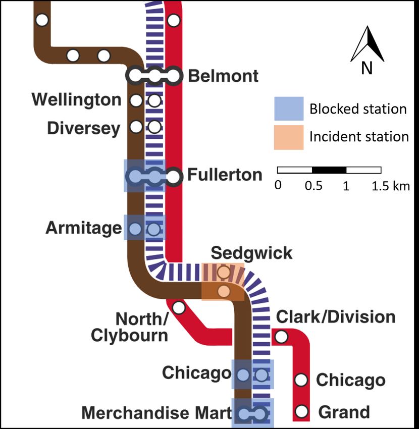
two real-world incidents in the CTA system. The corresponding policy implications and operation
      suggestions are also discussed.

    The remainder of this paper is organized as follows. Section 2 reviews the literature. Section 3 presents
the methodology used in this study. Case studies and data are described in Section 4 and results are discussed
in Section 5. Section 6 concludes the paper and discusses the policy implications.

2. Literature review

    There are generally four methods researchers use to analyze the impact of disrupted operations: graph
theory-based, survey-based, AFC data-based, and simulation-based. Graph theory-based analysis is majorly
used for supply network performance and supply service analysis. Survey and AFC data-based methods are
primarily used for passenger flows and individual behavior analysis. Lastly, simulation-based analysis can
be used for both supply and demand analysis. Each method has strengths and weaknesses depending on the
context.

2.1. Supply analysis
2.1.1. Network performance
    Network performance analysis usually uses graph theory-based techniques to identify key aspects of the
network’s properties related to incidents, such as resilience, redundancy, and vulnerability based on graph
theory (or complex network theory). For example, Yin et al. (2016) studied subway networks with respect
to disruptions, finding the weakness or critical locations of the network using “network betweenness” and
“global efficiency” metrics. Similarly, Zhang et al. (2018) built a general framework to assess the resilience
of large and complex metro networks by quantitatively analyzing their vulnerability and recovery time using
graph theory-based definitions.
    Simulation is also used to evaluate the impact of incidents on networks. Usually, different hypothetical
incident scenarios are tested. System performance metrics, such as travel delays and vehicle loads, are output
to analyze the incident effects. For example, Suarez et al. (2005) looked at the effects of climate change
on Boston’s transportation system performance using a simulation model, suggesting almost a doubling in
delays and lost transit trips due to a variety of climate change effects.
    Redundancy is an important indicators for analyzing the network performance under incidents. Redun-
dancy is best defined as “the extent to which elements, systems, or other units of analysis exist that are
substitutable, i.e., capable of satisfying functional requirements in the event of a disruption, degradation, or
loss of function” (Bruneau et al., 2003). Redundancy has been widely studied, not just for transportation
networks, but also in other areas including reliability engineering (O’Connor and Kleyner, 2012), commu-
nications (Wheeler and O’Kelly, 1999), water distribution systems (Kalungi and Tanyimboh, 2003), and
supply chain and logistics (Sheffi and Rice Jr, 2005). Transportation-specific resiliency and redundancy
studies include Berdica (2002), who developed a qualitative framework and basic concepts for vulnerability,
resilience, and redundancy. Other studies, like Wilson-Goure et al. (2006), Murray-Tuite (2006), and Good-
child et al. (2009), defined redundancy in the context of a specific transportation area of application. Jenelius

                                                        4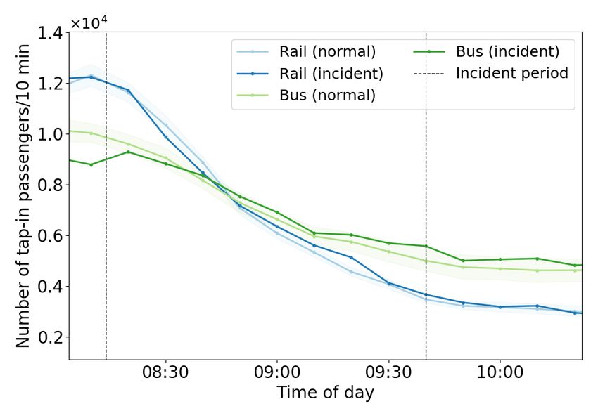
and Cats (2015) look at redundancy during line extensions. However, nearly all previous studies defined
redundancy for networks, links, and OD pairs. This study proposes an incident-based redundancy index
to evaluate the network’s ability to satisfy functional requirements under a specific incident. Both incident
location and duration impact the redundancy. Moreover, the bus system, which is an important alternative
for rail but rarely considered in previous studies, is included in the redundancy calculation.

2.1.2. Service Analysis
    Service analysis mainly focuses on changes in an agency’s operations during an incident period. This
type of analysis looks at headways, routing, staffing, shuttle services, and other operator-controlled factors
designed to mitigate the incident. For example, Nash and Huerlimann (2004) developed a simulation model
to analyze service variables such as headways and routing in the wake of disruptions. Schmöcker et al.
(2005) evaluated different operating strategies in six metro systems under service disruptions. Service delays
and recovering times are treated as performance indicators. Similarly, Mo et al. (2020a) proposed an event-
based simulation model that is capable of analyzing the impacts of incidents on service performance (e.g.,
headways).

2.2. Demand analysis
2.2.1. Passenger flow
    Passenger flow analysis focuses on understanding how passengers choose alternative services at an
aggregated level. Simulation-based methods can be applied to passenger flow analysis. For example, Hong
et al. (2018) simulated passenger flows in a metro station during an emergency. Using AFC data, Sun et al.
(2016) quantified three types of passenger flows: leaving the system, taking a detour, and continuing the
journey but being delayed. This model was applied to the Beijing metro network. Tian and Zheng (2018)
looked at unexpected train delay effects on Singapore’s MTR customers. Using AFC data, they built a
classification model to predict whether commuters switch from MRT to other transportation modes because
of unexpected train delays. Wu et al. (2020) used AFC data to detect passenger flow volumes and travel time
increases under station closures. Liu et al. (2021) uses AFC data to comprehensively analyze unplanned
disruption impacts, especially on passenger flows with trip cancellation, station changes, etc.

2.2.2. Individual behavior
    Individual behavior analysis usually focuses on individual responses, like mode choice, waiting time
tolerance, and a variety of other variables. These studies are usually conducted using surveys. Surveys are
a good means to understand individual choices. Revealed preference (RP) and stated preference (SP) are
two major types of survey design. Examples of transit-oriented RP studies include Currie and Muir (2017),
who conducted an RP survey to understand rail passengers’ behavior, perceptions, and priorities in response
to unplanned urban rail disruptions in Melbourne, Australia. Murray-Tuite et al. (2014) used a web-based
RP survey to understand the long-term impacts of a deadly metro rail collision in Washington DC. Tsuchiya
et al. (2008) conducted an RP survey in Japan that looked at passenger choices of four alternative routes.
Pnevmatikou and Karlaftis (2011) used RP survey data to analyze the effect of a pre-announced closure of
an Athens Metro Line. SP survey studies include Kamaruddin et al. (2012), who studied the modal shift

                                                      5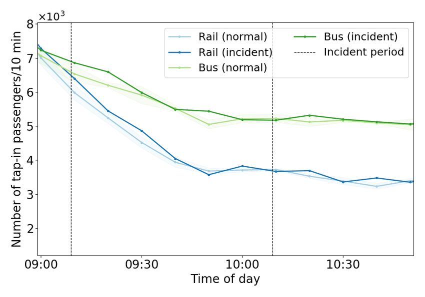
behavior of rail users after incidents. Fukasawa et al. (2012) investigated the effect of providing information
such as estimated arrival time, arrival order, and congestion level on passengers’ modal shift behavior in
response to an unplanned transit disruption. A similar research was conducted by Bai and Kattan (2014),
who found that various socioeconomic attributes and experience with the systems had strong influences on
travelers’ behavioral responses in the context of real-time information. Additionally, Rahimi et al. (2019,
2020) used an failure time model and a discrete choice model to analyze individuals’ waiting time tolerances
and mode choices, respectively, during unplanned service disruptions in Chicago using survey data.
    The major drawback of survey-based methods is that they are time-consuming and labor-intensive.
Hence, it is important to develop individual behavior analysis methods using AFC data as an alternative.

2.3. Comparison between our study and the literature
    Table 2 summarizes the various studies in the literature from three aspects: study methods, data sources,
and research focus. The main methodologies include graph theory-based methods (GTB), simulation-based
(SB), optimization models (OM), descriptive analysis (DA), statistical inference (SI), machine learning (ML),
and econometric models (EM).

                                       Table 2: Summary of literature review

Study                              Study Method    Data Sources                Research Focus
Yin et al. (2016)                  GTB             Network, AFC                1 NP- Efficiency
Zhang et al. (2018)                GTB             Network                     NP - Resilience
Balakrishna et al. (2008)          SB              Network, Survey             NP - Efficiency, Passenger flow, Service
Hong et al. (2018)                 SB              Synthetic                   Passenger Flow
Suarez et al. (2005)               SB              Network, Geographical       NP - Resilience
Mo et al. (2020a)                  SB, OM          Network, AFC                Passenger Flow, Service
Jenelius and Cats (2015)           SB              Network, AFC                NP - Redundancy
Adnan et al. (2017)                SB              Survey                      NP - Efficiency, Service
Schmöcker et al. (2005)            DA              AVL, AFC, Survey            NP - Resilience, Service
Sun et al. (2016)                  DA, SI          AFC                         Passenger Flow
Tian and Zheng (2018)              ML              AFC                         Delay
Wu et al. (2020)                   SI              AFC                         Passenger Flow
Liu et al. (2021)                  DA              AFC, AVL, Network           Passenger Flow, Delay
Currie and Muir (2017)             EM              Survey                      Travel mode choice, User satisfaction
Murray-Tuite et al. (2014)         EM              Survey                      Travel mode choice
Tsuchiya et al. (2008)             EM              Survey                      Travel mode choice
Pnevmatikou and Karlaftis (2011)   EM              Survey                      Travel mode choice
Kamaruddin et al. (2012)           EM              Survey                      Travel mode choice
Fukasawa et al. (2012)             EM              Survey                      Travel mode choice
Bai and Kattan (2014)              EM              Survey                      Travel mode choice
Lin et al. (2018)                  EM              Survey                      Travel mode choice
Pnevmatikou et al. (2015)          EM              Survey                      Travel mode choice
Rahimi et al. (2019)               EM              Survey                      Travel mode choice
Rahimi et al. (2020)               EM              Survey                      User waiting behavior
                                                                               Travel mode choice, Passenger flow,
Current study                      GTB, EM, DA     AFC, AVL, Network
                                                                               NP - Redundancy, Service
 1 NP:   Network performance.

                                                        6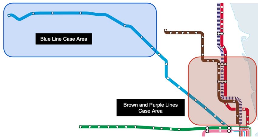
Our study presents a comprehensive analysis focusing on four aspects: travel mode choice, passenger
flow, redundancy, and service. It is also exclusive based on AFC and AVL data.

3. Methodology

    In this section, we present the building blocks and methods used to support the analysis framework of an
unplanned incident. On the supply side, a method to calculate the network redundancy index under a certain
incident is proposed, which reflects the network’s ability to provide alternative routes when incidents occur.
To analyze the agency’s service, we calculate the headway distribution using AVL data. On the demand side,
we describe how to analyze passenger flows under incidents using AFC data, and how to use AFC data to
analyze passengers’ mode choice using a binary logit model.
    To infer the effect of an incident, we compare data from the incident day to corresponding data from
normal days. A “normal day” is defined as a recent day with the same day of the week and there are no
incidents occurring in the incident line or nearby region during the incident period on that day. For example,
if an incident happened on Friday 9:00-10:00 AM at a station, normal days can be all Fridays in recent
months without incidents from 8:00-11:00 AM (a buffer is added to ensure normal services in a normal day)
on the same line. Headways and passenger flow during the incident day are compared to those of normal
days to reveal their difference.

3.1. Supply analysis
3.1.1. Network redundancy under incidents
    As mentioned in Section 2, since redundancy is used to evaluate a network’s functional response in the
event of disruptions, it is important to develop an incident-specific redundancy index (opposite to network,
link, or OD pair-specific in the literature). For a given incident, such an index can be used to evaluate the
network’s ability to provide alternative services under this incident. Furthermore, given the substitutional
relationship between bus and urban rail systems, the proposed redundancy index in this study also explicitly
considers the complementary role of bus and rail systems during the incident.
    Redundancy is usually a function of the number of available paths for each OD pair because more
available paths correspond to more opportunities of realizing the impacted trips when encountering service
disruptions (Xu et al., 2015). Hence, network redundancy under incidents (NRUI) should capture the
transport capacity of alternative paths during the incident. Typical path capacity is defined as the maximum
number of passengers transported per time unit (i.e. service frequency times the vehicle capacity). It is a
time-insensitive value, which means the travel times of paths are not considered. However, for the redundancy
calculation, path travel times are also important because passengers may not successfully finish their trips
during the incident period if they choose paths with a long travel time. This means that the time-insensitive
path capacity does not reflect the actual ability of paths to move passengers. Hence, a time-sensitive path
capacity should be used for the calculation. In this study, we propose a new metric for the calculation of
NRUI. The basis of the analysis uses the concept of throughput, instead of the classic definition of path
capacity. In our approach, throughput explicitly takes into account the travel time on each alternative path.
Throughput is defined as the number of “equivalent” passenger trips that have been completed per time unit

                                                      7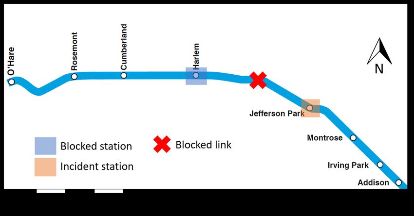
during the incident. If a passenger has completed half of the trip on an alternative path by the time an incident
is over, the “equivalent” trip count is 0.5.
     More specifically, let W be the set of all OD pairs of the rail network. For an OD pair w ∈ W, let Pw be
the set of available paths for w before the incident. As we consider both bus and urban rail systems, a path
p ∈ Pw may include segments of bus trips. Pw can be obtained in several ways, such as route choice surveys,
Google Map API, and k-shortest paths. In this study, k-shortest path is used to obtain Pw with additional
manual tuning to filter out unrealistic paths (e.g., too many transfers). Let DI be the duration of incident I,
Hp the headway of path p (defined as the maximum headway of each segment of path p), Cp be the vehicle
(i.e. train or bus) capacity of path p (defined as the minimum vehicle capacity over all segments of path p),
and Lp the travel time of path p. Then bDI /Hp c is the total number of vehicles dispatched on path p during
the incident period. The throughput aims to capture the number of passengers at various stages of completing
their trips during the incident. Figure 1 illustrates how the equivalent number of passengers completing trips
are calculated during the incident period. If DI < Lp (Figure 1a), all vehicles in the path cannot reach the
final destination. Therefore, the number of transported passengers is counted proportionally based on their
travel time in the vehicle. For example, the first vehicle has traveled for DI during the incident period (i.e.
DI
Lp   of the total path length). We assume this is equivalent to Cp DI
                                                                   Lp completed passenger trips. And it is easy
                                                                                                         DI −(k−1)Hp
to show that the k-th vehicle’s travel time is DI −(k −1)Hp , which corresponds to Cp                         Lp         equivalent
completed passenger trips during the incident period. If DI ≥ Lp (Figure 1b), the first vehicle can reach the
destination. So it accounts for Cp completed passenger trips. In the example shown in Figure 1b, the second
vehicle can also reach the destination during the incident (accounting for Cp passenger trips), while the third
                                 DI −2Hp
cannot (accounting for Cp           Lp     passenger trips). Therefore, combining these two scenarios, the number
                                                                                            min {DI −(k−1)Hp ,Lp }
of equivalent completed passenger trips for vehicle k can be calculated as                           Lp               · Cp .

                          (a) DI < Lp                                                        (b) DI ≥ Lp

Figure 1: Illustration of path throughput. The bars show the number of equivalent completed passenger trips during the incident
period (unfinished trips are counted proportionally based on their travel time). The orange (blue) bars represent vehicles that cannot
(can) finish the trips.

                                                                  8
Let Ap be the throughput of path p under incident I. From the analysis above, it can be formulated as
bDI /Hp c
1 X min {DI − (k − 1)Hp , Lp }
Ap = · Cp (1)
DI Lp
k=1
Eq. 1 counts the total number of equivalent passenger trips along path p that have been completed per time
unit during the incident (passengers who did not finish their trips are counted proportionally).
A larger value of DI implies that Ap is less sensitive to the path travel time. On the extreme situation
Cp
where DI → ∞, Ap → Hp (proof in Appendix A), which corresponds to the typical definition of capacity
where Lp does not matter. The intuition behind this is that the proposed Ap limits the capacity calculation
in the incident period. When DI is large, even if passengers have a longer travel time on a path, the majority
of the passengers impacted by the incident will have their trips completed. So the travel time is not very.
On the contrary, if DI is small, most of the passengers using paths with long travel times cannot finish their
Cp
trips. The typical definition of Hp does not capture this important aspect. Hence, considering travel time in
the redundancy calculation is much more representative of the actual conditions.
In summary, Ap is an indicator reflecting a path’s ability to serve impacted trips during the incident
P
period. And p∈Pw Ap reflects the ability of the network to provide services for OD pair w. Actually, one
P P
of the network-level definitions of redundancy in the literature is w∈W p∈Pw Ap (where Ap is defined
differently), which measures the total path capacity in the network (Leistritz et al., 2013).
In this study, we want to capture the incident-specific characteristics of redundancy. Let WI be the set
of all OD pairs with at least one path blocked due to incident I. Mathematically, WI = { w ∈ W : ∃p ∈ Pw
s.t. p is blocked due to incident I }. Then, only passengers with OD in WI are affected by the incident. Let
the total path throughput of w before the incident be Tw .
X
Tw = Ap ∀w ∈ WI (2)
p∈Pw
Because of the incident, passengers may augment their typical path choice alternatives with paths that
were not considered before the incident. Hence, we define P̃w as the set of available paths for w ∈ WI during
the incident. P̃w can be seen as Pw without the blocked paths and adding the augmented paths. Usually,
augmented paths are longer and less preferred by passengers. For a specific OD pair w ∈ WI , the total path
throughput of w after the incident, denoted as T̃w , should be less than or equal to that before. Therefore, we
define T̃w as:
X
T̃w = min{ Ap , T w } ∀w ∈ WI (3)
p∈P̃w
This corresponds to our assumption that the throughput during the incident cannot exceed that before the
9incident for a specific OD pair. Hence, the NRUI for incident I is formulated as:
P
w∈WI T̃w
RI = P (4)
w∈WI Tw
where the numerator (denominator) is the total throughput of available paths after (before) the incident.
Since Tw ≥ T̃w for all w ∈ WI by definition, we have 0 ≤ RI ≤ 1. RI = 1 means the capacities before and
after the incident are the same, suggesting that the incident does not deteriorate the function of the network
(i.e. the network is fully redundant under incident I). RI = 0 means no alternative paths are available
during the incident (i.e. the network has no redundancy under incident I)
For better understanding of the index, we present a small numerical example to show how RI is calculated.
As shown in Figure 2, consider a system with only one OD pair w. Path 1 and 2 are primary and alternative
paths, respectively, where Pw = {1} and P̃w = {2} (i.e. before the incident path 2 is not chosen by
passengers). The attributes of two paths are shown in the figure. For path 1, there are bDI /Hp c = 2 vehicles
dispatched. The first vehicle has traveled for min{DI , L1 } = 20 minutes and reached the destination.
The second vehicle, which was dispatched 30 minutes later, can also travel for min{DI − H1 , L1 } = 20
minutes and reach the destination. Therefore, these two vehicles successfully carried 400 passengers to the
destination. According to Eq. 1, we have
min{DI , L1 } min{DI − H1 , L1 }
A1 = C1 + C1 = 400 passengers/hour (5)
L1 DI L1 DI
In terms of path 2, similarly, there are two vehicles dispatched during the incident. The first vehicle can
30
reach the destination and the second one can only finish 60 of its journey. Therefore,
min{DI , L2 } min{DI − H2 , L2 }
A2 = C2 + C2 = 300 passengers/hour (6)
L2 DI L2 DI
The two terms in Eq. 6 represent the number of passengers carried (successfully and partially) by the two
vehicles in path 2 per time unit.
The redundancy index for this single network under incident I is
T̃w A2 300
RI = = = = 0.75 (7)
Tw A1 400
which means during the incident when passengers start to use path 2, the system maintains 75% of its original
capacity. For comparison purpose, if one follows the typical definition of path capacity and calculate Ap as
Cp
Hp , the redundancy index will be 1 because C1 = C2 and H1 = H2 in this example, which is obviously
unreasonable because it implies that the system maintains 100% capacity and the incident has no impact.
10Figure 2: Example of network redundancy calculation
It is worth noting that we illustrate the definition of the NRUI assuming a fixed vehicle capacity Cp .
Actually, Cp can be defined as the “available capacity” in a vehicle considering the onboard passengers. In
this way, the NRUI can also capture the impact of demand. The “available capacity” can be calculated
for the specific day of the incident using a transit assignment model (Mo et al., 2020a). Alternatively, the
average “available capacity” can also be used. In the case study, due to lack of data, the total capacity of a
vehicle is used.
3.1.2. Headway analysis
Headways are important indicators of the level of service for transit systems. Analyzing headway
patterns during an incident can provide direct information about how services are reduced by the incident.
As mentioned in Section 1, AVL data provide the headway of each station in the urban rail system. In this
study, we calculate the headway temporal distribution for lines of interest to capture the impact of incidents.
Let us divide the analysis time period into several intervals with equal length. Denote the headway on
station i of trip j as Hi,j (i.e. the length of interval between trip j and j − 1 and Hi,1 = 0). Suppose line l
has two directions, inbound and outbound. The headway of line l outbound at time interval τ is calculated
as
P P
i∈Slout j∈Ri,τ Hi,j
out
Hl,τ = P (8)
i∈Slout |Ri,τ | − 1
where Slout is set of outbound stations in line l. Ri,τ is the set of trips passing through station i during
the time interval τ . Eq. 8 implies the headway of a line is calculated as the mean of all stations along the
in , is calculated in a similar way by replacing S out with S in . The headway
line. The inbound headway, Hl,τ l l
distributions of both normal days and the incident day are calculated for comparison.
3.2. Demand analysis
3.2.1. Passenger flow analysis
AFC data record passengers’ tap-in information in bus and rail systems (tap-out is not available in
this study). These transactions can capture passengers’ route choices during an incident if they use the
transit system again (Mo et al., 2020b). Therefore, analyzing AFC data can help understand passenger flow
redistribution during an incident.
11At the station level, we calculate the number of tap-in passengers at the stations in the incident area,
and compare the values on the incident day and normal days. The difference in this number is an indicator
of the impact of the incident on passenger flow redistribution. Stations with high demand increase reflect
passengers’ choices after the incident. Similarly, at the line level, we calculate the number of tap-in passengers
for lines near the incident area for both the incident day and normal days. Line-level demands are calculated
as the sum of all station-level demands in corresponding lines.
Note that we assume the number of tap-in passengers is approximately normally distributed. Hence, if
the incident day demand is beyond the ±2×standard deviation of the normal day demand, we say that a
significant difference is observed (i.e., the impact of the incident is significant).
3.2.2. Individual behavior analysis
Passengers may make different mode choices after the incident. One important question is how the
characteristics of the passengers influence their mode choices. This is typically using data from surveys. In
this study, we propose a method based on conveniently available AFC data for individual behavior analysis.
The proposed approach consists of two steps: a) inferring individual’s mode choice and b) extracting
samples’ characteristics. We infer individual choices using AFC data. In this study, only two choices are
considered: 1) using transit and 2) other (including canceling trips and using other travel modes). This is
because these two options can be confidently identified using AFC data and they are important for transit
operators. Since passenger travel patterns in transit systems show high irregularity (Goulet-Langlois et al.,
2017), it is more convenient to identify the behavioral changes of regular passengers (Mojica, 2008). In
this study, we define regular passengers as those who use the public transit system every normal day and
have the same travel trajectories. Note that, as normal days have the same day of week as the incident
day, regular passengers are not necessarily frequent users as they may only use the system on a specific
day of week. For example, if an incident happened on Friday, a passenger who only uses the public
transit system on Friday (i.e. on each normal day) is a regular passenger. But since he/she only uses
the transit once a week, he/she may not be a frequent user. Mathematically, let us denote the trajectories
of passenger i in normal day k as T i,k = {(oi,k i,k i,k i,k i,k i,k i,k i,k
1 , d1 , t1 ), ..., (oN i,k , dN i,k , tN i,k )}, where on , dn , and
ti,k i,k i,k
n are the origin, destination and start time of the n-th trip, respectively (t1 < ... < tN i,k ). N
i,k is
the total number of trips in normal day k for passenger i. The set of regular passengers is defined as
0 0 0
{i ∈ I | oi,k i,k i,k i,k i,k i i i i
n = on , dn = dn , tn ∈ [t̄n − σn , t̄n + σn ], N
i,k = N i,k , ∀k, k 0 ∈ K, k 6= k 0 }, where I is
the set of all passengers, t̄in and σni are the mean and standard deviation of the start time of trip n for passenger
i over all normal days. K is the set of all normal days considered in this study. This means regular passengers
have the same number of trips and corresponding origins and destinations in each normal day (for tap-in
only AFC systems, destinations are not considered). And the corresponding trip start times in each normal
day are stable (i.e. within a standard deviation). Hence, if these passengers had different travel patterns on
the incident day, most likely they would be affected by the incident and chose a new travel mode. Denote
the trip sequence of passenger i on the incident day as T i,In = {(oi,In i,In i,In i,In i,In i,In
1 , d1 , t1 ), ..., (oN i,In , dN i,In , tN i,In )}.
And let [Te , Ts ] be the incident period, where Te and Ts is the incident start and end time. The mode choice
during the incident for a regular passenger i is denoted as Yi . We infer Yi as follows:
12• Yi = “Transit” if 1) there are additional transit trips (compared to that in a normal day) during the
incident period or 2) there are changes of tap-in stations during the incident period. The first condition
implies that the regular passenger may have transferred to a nearby rail station or bus stop, with more
transit trips than usual. The second condition implies that the regular passenger may have changed to
a different rail line or bus route in response to the incident. Let TIi,k = {(oi,k i,k i,k
n , dn , tn ) ∈ T
i,k | T ≤
s
t̄in ≤ Te } and TIi,In = {(oi,In i,In i,In
n , dn , tn ) ∈ T
i,In | T ≤ ti,In ≤ T } be sub-sequences of trips within
s n e
the incident period (i.e. [Ts , Te ]) on a normal and the incident day, respectively. Mathematically,
the first condition can be expressed as: |TIi,In | > |TIi,k | and the second: ∃n s.t. oi,k i,In
n 6= on , where
(oi,k i,k i,k
n , dn , tn ) ∈ TI
i,k
and (oi,In i,In i,In i,In
n , dn , tn ) ∈ TI . Note that k ∈ K can be any normal day because
the trajectories for all normal days are the same for a regular passenger by definition.
• Yi = “Other” if the transit trips that are supposed to happen during the incident period on the normal
days disappear on the incident day. This means that the regular passengers may change to other modes
or cancel their trips. Mathematically, this can be expressed as |TIi,In | < |TIi,k |.
Other regular passengers without the above behavior may not be affected by the incident or have other
choices that are hard to be identified (e.g., transfer to another line without leaving the system), which are not
considered in the analysis.
In the second step, the characteristics of each regular passenger (i.e. demographics and trip information)
are extracted. We aim to use information that is available in AFC and sale transaction data as a proxy to
passengers’ socio-demographics.
Since regular passengers have consistent travel trajectories, we can infer their home locations as the tap-in
rail station or bus stop of the first trip on a normal day (i.e. oi,k
1 for any k ∈ K). Given the station/stop location,
we can obtain the median household income in passenger i’s neighborhood or census tract using census data.
Living in a high-income or low-income neighborhood can be a proxy of passengers’ income. AFC data can
also provide passengers’ fare status information, such as whether the passenger is in a reduced fare status.
Reduced fare status users are usually students, seniors, and people with disabilities. This information is also
a proxy for socio-demographic characteristics.
Sale transaction data provide the historical add-value transactions of passengers. We extract three
variables in this study: total added value per year, add-value frequency (i.e. number of add-value transactions
per year), and maximum single added value in a year. The first two variables reflect the passenger’s
dependence on and familiarity with public transit and part of their income information. The last variable can
also be used to some extent as a proxy for income because low-income people may not be able to deposit a
large amount of money in the smart card at once. We denote all this “proxy” demographic information for
passenger i as Xi .
The characteristics of passenger i’s trip (denoted as Zi ) during the incident may also affect mode choices.
We define the incident-related trip (trip ID denoted as n∗ ) as the first trip with t̄i,k in the incident period.
Mathematically, n∗ = arg minn {n = 1, ..., N i,k | t̄in ∈ [Ts , Te ]}. Since regular passengers are supposed
to have stable travel patterns, oi,k i,k
n∗ and dn∗ should be the intended origin and destination for passenger i on
the incident day. Based on (oi,k i,k
n∗ , dn∗ ), two trip-related variables are considered. The first is whether the
di,k i,k
n∗ is downtown, which is a proxy for work trips. Note that for a tap-in only system, dn∗ can be inferred
13from a destination estimation model (Barry et al., 2002; Zhao et al., 2007; Gordon et al., 2013). The second
variable is OD-based redundancy, defined as
T̃wi
RiOD = (9)
Twi
where RiOD is the OD-based redundancy for passenger i, measuring the availability of alternative transit
services for the specific OD pair during an incident. wi = (oi,k i,k
n∗ , dn∗ ) is passenger i’s OD pair for the
incident-related trip. It is worth noting that RiOD can be seen as the NRUI for the case of a single OD pair.
In this study, we use a binary logit model (Ben-Akiva et al., 1985) to better understand the main factors
that impact choice Yi . Let the utility of mode j for passenger i be Uij .
Uij = ASCj + αj Xi + βj Zi + j (10)
where ASCj is the alternative specific constant (ASC) for mode j. j is the error term that is assumed to be
Gumbel distributed. αj and βj are the vectors of parameters to be estimated. The probability of passenger i
choosing mode j is
exp(ASCj + αj Xi + βj Zi )
P(Yi = j) = P ∀j ∈ C (11)
j 0 ∈C exp(ASCj + αj Xi + βj Zi )
where C = {“Transit”, “Other”} is the choice set.
The approach of the individual behavioral analysis model is summarized in Figure 3.
Figure 3: Summary of the individual behavioral analysis model
4. Application
4.1. Chicago Transit System
We use incident data from the Chicago Transit Authority (CTA) public transit system for the model
application in this section. CTA is the second-largest transit system in the United States, providing services
in Chicago, Illinois, and some of its surrounding suburbs. It operates 24 hours each day and is used by 0.84
million bus and 0.81 million train passengers per weekday on average (CTA, 2019). The map of the CTA rail
system is shown in Figure 4. The rail system consists of eight lines (named after their color) and the "Loop".
The Loop, located in the Chicago downtown area, is a 2.88 km long circuit of elevated rail that forms the
14hub of the Chicago rail system. Its eight stations account for around 10% of the weekday boardings of the
CTA trains.
Figure 4: CTA rail system map
CTA’s AFC system is entry-only, meaning passengers use their farecards only when entering a rail station
or boarding a bus, and so no information about a trip’s destination is directly provided. The train tracking
system provides train arrival and departure times at each station.
According to the control center data, CTA experienced a total of 27,198 incidents in 2019. However,
around 80% percent of the incidents have a duration of fewer than 10 minutes. Since small incidents may
not affect the system significantly, this study focuses on substantial incidents that lasted longer than 1 hour.
Passengers who leave the rail system because of service disruptions need to re-tap in if they decide to use
other CTA services (buses or rails). They are only charged a transfer fee. However, no tap-in is needed for
shuttle service that may have been deployed in response to the incident. Hence, there is no information for
passengers using shuttle buses.
4.2. Redundancy index
Prior to analyzing actual incidents, we first present an overview of the CTA system redundancy. As
the NRUI is defined based on each incident, for the purpose of this analysis, we assume that a hypothetical
incident takes place at a station in the system (one at a time), blocking the track segment that connects the
station for 1 hour. Note that if a station has two separate tracks, each track is blocked independently and there
will be two incident cases for this station. For example, the Roosevelt station has two different tracks for the
Red Line and Purple/Yellow Lines. So two hypothetical incident cases are generated, each corresponding
to the interruption of a track. Considering the infrastructure layout of urban rail systems, assuming that
incidents occur at the track level is more realistic than simply assuming an incident blocks the whole station
as in many previous studies that used graph-based methods (Chopra et al., 2016; Ye and Kim, 2019).
Besides the incident-specific redundancy index, the occurrence frequency of incidents at various stations
is also of importance. Figure 5 shows the redundancy index at each station against the number of incidents
taking place per year at that station (only incidents with a duration greater than 10 minutes are counted). The
15combination of the two metrics divides the figure into four sections: 1) Stations in the red section (upper left)
have high incident occurrence frequency and low redundancy. These are critical stations in the system where
alternative public transit services are limited and service disruptions happen frequently. Transit operators
need to prepare strategies in advance for these stations. 2) Stations in the yellow section (upper right) have
high incident occurrence frequency and high redundancy. In these stations, passengers are able to seek
alternative services during a disruption. Operators need to provide direct information to passengers with
suggestions regarding alternatives. 3) Stations in the blue section (lower left) have low incident occurrence
frequency and low redundancy. Though incidents may not happen frequently, mitigation plans need to be
prepared as there are limited substitutional services. 4) Stations in the green section (lower right) have low
incident occurrence frequency and high redundancy. These stations are less critical in terms of incident
management compared to stations in other sections.
Figure 5 shows that most of the stations in the CTA system are in the blue or green sections. And only
a limited number of stations are in the red section. This implies that CTA can focus more on some critical
stations with adequate incident management strategies. In terms of critical stations (red section), most of
them are terminal stations (such as Howard, Forest Park). This is expected as terminal stations usually have
more complex infrastructure layouts (i.e. more prone to failures) and are usually located in suburban areas
(i.e. fewer alternative services and low redundancy index). Backup shuttle services can be provided in these
stations.
Figure 5: Redundancy index v.s. incident occurrence rate.
4.3. Rail disruption cases
Since the location of the incidents may influence their impact, we selected two incidents at locations with
high and low redundancy, respectively, for comparative analysis.
164.3.1. Brown and Purple Lines Sedgwick incident
On September 24 (Tuesday), 2019, at 9:09 AM, a Purple Line train collided with a Brown Line train at
the Sedgwick station. The incident caused a number of stations to be blocked and closed in both Brown and
Purple Lines since these two lines share the same track in this area. The impacted stations were Fullerton
and Armitage to the north and Chicago and Merchandise Mart (MM) to the south. Southbound trains short
turned at Fullerton, while northbound trains short turned at MM. At 9:28 AM, 19 minutes after the incident
started, bus substitution service began between Fullerton to MM. Service resumed at all blocked stations at
10:19 AM, 70 minutes after the start of the incident. The incident on the Brown and Purple Lines is a high
redundancy case because the Red Line is a good substitution for the incident location (See Figure 6).
Figure 6: Incident diagram of Brown Line Sedgwick case
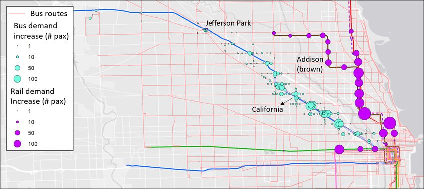
4.3.2. Blue Line Jefferson Park incident
On February 1 (Friday), 2019, at 8:14 AM, the inbound track Blue Line between Harlem and Jefferson
Park was closed due to infrastructure problems. All trains in the Blue Line were suspended. CTA used
the remaining single-direction track to serve trains from both directions in the incident link. At 9:03 AM,
49 minutes after the incident, single track operations commenced between Harlem and Jefferson Park, with
shuttle service starting 7 minutes later. At 9:40 AM, all inbound trains succeeded to move under the single-
track operation. At 12:09 PM, the full line was reopened. The entire incident lasted 4 hours and 9 minutes.
The incident on the Blue Line is a low redundancy case because the Blue Line is far away from other rail
lines with limited alternative services (see Figure 7).
17Figure 7: Incident diagram of Blue Line Jefferson Park case
5. Analysis
The framework discussed in Section 3 was used for the analysis of the cases. For each case, the results
are organized from supply to demand analysis. The individual choice analysis is conducted based on samples
of affected passengers from two incidents.
5.1. Brown and Purple Line incident analysis
5.1.1. Redundancy index
The NURI (Eq. 4) for the Brown and Purple Line case is 0.732, meaning that the transit system maintains
73.2% transporting capacity for the Brown and Purple Lines incident during the incident period. The high
redundancy of the Brown and Purple Lines incident is as expected. In the incident area, the Red Line is
almost parallel with the Brown and Purple Lines. In addition, there exist many south-bound bus routes going
to Downtown Chicago (see Figure 11). This implies that during the Brown and Purple Line incident, CTA
can focus on guiding passengers to find alternative services. Some information dissemination strategies need
to be applied, such as route and transfer recommendations.
5.1.2. Headway analysis
The headway analysis results from the Brown and Purple Line Sedgwick incident are summarized in
Figure 8. The shade around normal day lines indicates ±standard deviation (same for all the following
figures with shades around normal day lines). The line-level headway is calculated as Eq. 8. We selected
three lines with directions of interest to analyze. Recall that the Brown and Purple Lines share tracks in the
incident area, while the Red Line runs on separate tracks in the incident area but shares tracks further north
of the line.
18(a) Brown Line (southbound) (b) Purple Line (southbound) (c) Red Line (southbound)
Figure 8: Headway temporal distribution (Brown and Purple Lines Sedgwick incident). The shade around normal day lines indicates
±standard deviation (same for all following figures)
A rise in southbound headways for both the Brown and Purple Lines are observed (Figures 8a and 8b)
and the changes are significant (i.e., beyond the two standard deviation range). This is as expected because
these two lines are blocked due to the incident. On average, headway increases from 5 minutes to 15 minutes
in Brown Line and from 5 minutes to 7 minutes in Purple Line, implying a reduction of service frequency
by 66.7% and 28.6% for Brown and Purple Lines, respectively. The Brown Line experiences a continuous
increase in headways towards the end of the incident. And we see a decrease in headways once the incident
clears. The Purple Line, which has most of its local stops farther away from the incident area, has less
disrupted service at the line level, despite sharing tracks with the Brown Line. So its headways deviated less
from the normal-day average.
As shown in Figure 8c, the Red Line experiences little deviation from its normal day service for the first
half of the incident (before 9:30 AM), largely because it does not share tracks at the incident location and
could run largely uninterrupted. However, halfway through the incident, there is a headway increase spike.
This could be caused by two possible reasons: 1) Because of the bad service on Brown and Purple Lines,
passengers chose to take the Red Line southbound instead, leading to more passengers and thus the delays
at the stations when loading and unloading passengers. 2) The unusual operation (e.g., short-turn) of the
trains on Brown and Purple Lines may occupy facilities in the Red Line, resulting in congestion and longer
headways. The headway increase in nearby lines implies that the transit operator should pay attention to both
incident lines and nearby lines to better serve passengers.
5.1.3. Passenger flow analysis
Passenger flows can be examined at multiple levels, including system-wide, line level, and station level.
Figure 9 shows the total number of tap-in passengers for the bus and rail systems during the Brown and Purple
Lines incident. The results show that there is no significant difference between the incident day and normal
days for both bus and rail because the demand lines on the incident day are within the ±2 standard deviation
range. This implies that though the incident lasted for more than 1 hour and blocked several stations, the
impact on the whole system demand is still negligible (i.e., as influential as the inherent demand variations).
19Figure 9: System level passenger flow analysis (Brown and Purple Lines incident).
The line-level demand changes for the Brown and Purple Line incident are shown in Figure 10. As
expected, demand on the Brown and Purple Lines (interrupted by the incident) both decreased during the
incident and returned to normal after the incident. And the decrease is significant. As the Red Line runs
adjacent to the Brown and Purple Lines for a significant portion and is not suspended, we see a significant
increase in demand during the incident period with a return to normal after the incident is over.
(a) Brown Line (blocked) (b) Purple Line (blocked) (c) Red Line (open)
Figure 10: Line level passenger flow analysis (Brown and Purple Lines incident)
We further examine the demand changes at rail and bus stations close to the incident area (shown in
Figure 11). During the incident, we see an increase in rail demand at Fullerton and Belmont stations that
have direct connections to the uninterrupted Red Line. We also see clusters of increased bus demand near
the incident lines. Of note are the clusters outlined in red and blue squares. The red clusters represent
increased bus demand proximal to blocked stations. These passengers may have transferred directly to
nearby bus stops from the blocked line. Additionally, the blue clusters represent increases in bus demand for
routes that connect directly to downtown. The increase may be attributed to passengers who live in nearby
neighborhoods and change to buses during the incident.
20The total decrease in the number of tap-in passengers in the Brown and Purple Lines is 1,141, while
the increase in nearby bus stations and the Red Line is 696 and 1,414, respectively. The demand decrease
in the Brown and Purple lines is smaller than the corresponding increase in the Red Line and bus stations.
This is probably because some passengers may first tap in the Brown and Purple Lines and then leave
(this phenomenon will be illustrated in Figure 12), which leads to the underestimation of demand decrease
in Brown and Purple Lines. For all the 2,110 observed passengers using the alternative services, around
one-third of them (696) transfer to buses and two-thirds (1,414) to the Red Line. Note that there may also be
many passengers with direct transfers without leaving the system, which cannot be observed from the AFC
data.
Figure 11: Station demand increase patterns (Brown and Purple Lines incident)
Additionally, Figure 12 shows the temporal demand distribution at three stations: Sedgwick (the incident
station), Fullerton (a nearby partially blocked station), and North/Clybourn (a nearby station in Red Line that
is open). The illustrated trends align with the incident pattern. At Sedgwick (Figure 12a), the center of the
incident, we see a drastic decrease in demand once the incident starts. As some passengers may not be aware
of the incident and accidentally tapped into the station, the demand is not zero during the incident period.
After the incident is over, we see a quick recovery in demand. In terms of the Fullerton (Figure 12b) station,
despite it being partially blocked (the tracks of Brown/Purple Lines are blocked but the track of Red Line are
not), we see an immediate rise in demand. This indicates that passengers used Fullerton station for the Red
Line. Lastly, we see a sharp increase in the number of tap-in passengers at the North/Clybourn station in the
Red Line (Figure 12c), which is within walking distance from Sedgwick station. This implies that passengers
from the Brown and Purple Lines may also walk to the Red Line to finish their journey. Additionally, this
station gives passengers access to Fullerton station, where they can switch to Brown or Purple Lines trains
going northbound. The sharp increase may represent the first wave of transfer passengers.
21You can also read