Two-channel system dynamics of the outer Weser estuary - a modeling study
←
→
Page content transcription
If your browser does not render page correctly, please read the page content below
Article, Published Version

Gundlach, Jannek; Zorndt, Anna; van Prooijen, Bram C.; Wang, Zheng
Bing
Two-channel system dynamics of the outer Weser estuary
– a modeling study
Journal of Marine Science and Engineering

Verfügbar unter/Available at: https://hdl.handle.net/20.500.11970/107500

Vorgeschlagene Zitierweise/Suggested citation:
Gundlach, Jannek; Zorndt, Anna; van Prooijen, Bram C.; Wang, Zheng Bing (2021): Two-
channel system dynamics of the outer Weser estuary – a modeling study. In: Journal of
Marine Science and Engineering 9 (4). S. 448.

Standardnutzungsbedingungen/Terms of Use:

Die Dokumente in HENRY stehen unter der Creative Commons Lizenz CC BY 4.0, sofern keine abweichenden
Nutzungsbedingungen getroffen wurden. Damit ist sowohl die kommerzielle Nutzung als auch das Teilen, die
Weiterbearbeitung und Speicherung erlaubt. Das Verwenden und das Bearbeiten stehen unter der Bedingung der
Namensnennung. Im Einzelfall kann eine restriktivere Lizenz gelten; dann gelten abweichend von den obigen
Nutzungsbedingungen die in der dort genannten Lizenz gewährten Nutzungsrechte.
Documents in HENRY are made available under the Creative Commons License CC BY 4.0, if no other license is
applicable. Under CC BY 4.0 commercial use and sharing, remixing, transforming, and building upon the material
of the work is permitted. In some cases a different, more restrictive license may apply; if applicable the terms of
the restrictive license will be binding.
Journal of
               Marine Science
               and Engineering

Article
Two-Channel System Dynamics of the Outer Weser
Estuary—A Modeling Study
Jannek Gundlach 1, *, Anna Zorndt 2 , Bram C. van Prooijen 3 and Zheng Bing Wang 3,4

                                          1   Ludwig-Franzius-Institute for Hydraulic, Estuarine and Coastal Engineering, Leibniz University Hannover,
                                              30167 Hanover, Germany
                                          2   Federal Waterways Engineering and Research Institute (BAW), 22559 Hamburg, Germany;
                                              anna.zorndt@baw.de
                                          3   Faculty of Civil Engineering and Geosciences, Delft University of Technology,
                                              2628 CN Delft, The Netherlands; B.C.vanProoijen@tudelft.nl (B.C.v.P.); z.b.wang@tudelft.nl (Z.B.W.)
                                          4   Deltares, P.O. Box 177, 2600 MH Delft, The Netherlands
                                          *   Correspondence: gundlach@lufi.uni-hannover.de

                                          Abstract: In this paper, we unravel the mechanisms responsible for the development of the two-
                                          channel system in the Outer Weser Estuary. A process-based morphodynamic model is built based
                                          on a flat-bed approach using simplified boundary conditions and accelerated morphological develop-
                                          ment. The results are analyzed in two steps: first, by checking for morphodynamic equilibrium in the
                                          simulations and second, by applying a newly developed method that interprets simulations based
                                          on categorization of the two-channel system and cross-sectional correlation analysis. All simulations
                                          reach a morphodynamic equilibrium and develop two channels that vary considerably over time
                                          and between the simulations. Variations can be found in the location and depth of the two channels,

                                   the development of the dominant channel over time and the alteration in the dominance pattern. The
Citation: Gundlach, J.; Zorndt, A.;       conclusions are that the development of the two-channel system is mainly caused by the tides and
van Prooijen, B.C.; Wang, Z.B.            the basin geometry. Furthermore, it is shown that the alternation pattern and period are dependent
Two-Channel System Dynamics of the        on the dominance of the tides compared to the influence of river discharge.
Outer Weser Estuary—A Modeling
Study. J. Mar. Sci. Eng. 2021, 9, 448.    Keywords: morphodynamics; Delft3D; long-term; two-channel
https://doi.org/10.3390/jmse9040448

Academic Editors: Pushpa
Dissanayake, Jenifer Brown and            1. Introduction
Marissa Yates
                                                The Weser estuary is one of the four estuaries in the German Bight. Its morpho-
                                          logical pattern is characterized by a distinctive two-channel system in the Outer Weser
Received: 10 March 2021
Accepted: 15 April 2021
                                          part. This characteristic is relevant for the navigational access to the ports of Bremen and
Published: 20 April 2021
                                          Bremerhaven [1]. In the late 19th century, a combination of increased navigational depth
                                          requirements and the limitation of navigational space due to morphological alternations [2]
Publisher’s Note: MDPI stays neutral
                                          led to the construction of training walls and groynes [3,4] plus capital dredging [5]. Those
with regard to jurisdictional claims in
                                          anthropogenic interventions minimized the natural fluctuations in the position and dimen-
published maps and institutional affil-   sions of the two-channel system and permanently constrained the marine traffic to the
iations.                                  main channel.
                                                Morphology of estuaries and tidal inlet is governed by a complex combination of
                                          influences [6]. Roelvink and Reniers [7] question the scale/degree to which an estuarine
                                          bathymetry is forced by its own boundaries, such as dikes, headlands, unerodable layers,
Copyright: © 2021 by the authors.
                                          natural or man-made constraints. The most intrusive bathymetrical pattern is the appearance
Licensee MDPI, Basel, Switzerland.
                                          of tidal channels and shoals. Each estuary and tidal inlet has an individual arrangement of
This article is an open access article
                                          tidal features based on its forcing [8]. Nevertheless, large-scale features, such as the main
distributed under the terms and           channel(s), dividing shoals or branching side-channels, can be found commonly [9,10].
conditions of the Creative Commons              The advances in numerical modeling software [10–13] and rising computational ca-
Attribution (CC BY) license (https://     pacity allow detailed morphodynamic investigations [7,14] and long-term morphodynamic
creativecommons.org/licenses/by/          simulations [15–17]. With these capacities given, it is now feasible to investigate reasons of
4.0/).                                    the development of a two-channel system and morphodynamic alternations.

J. Mar. Sci. Eng. 2021, 9, 448. https://doi.org/10.3390/jmse9040448                                            https://www.mdpi.com/journal/jmse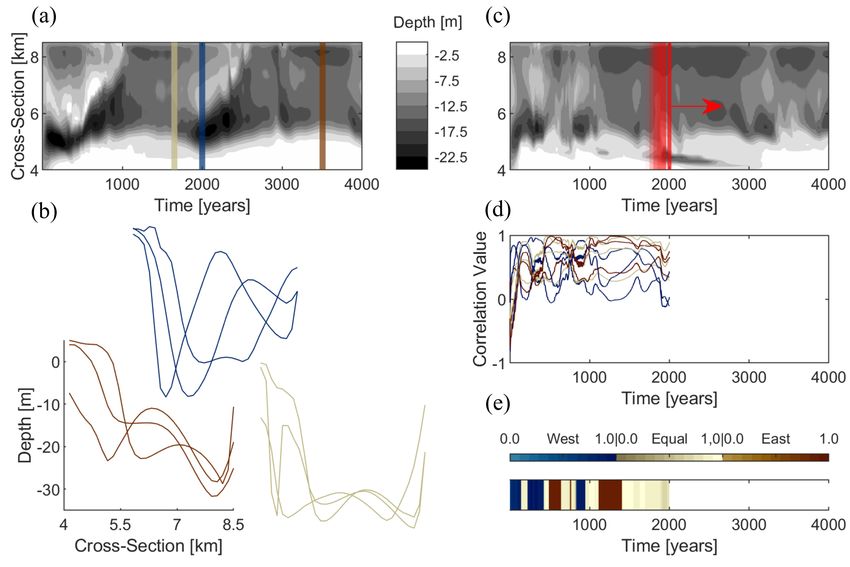
J. Mar. Sci. Eng. 2021, 9, 448                                                                                             2 of 21

                                       Contrary to systems like the Western Scheldt [18,19], not many numerical studies
                                 about the morphodynamics of the Weser Estuary have been published. Herrling et al. [20]
                                 investigated the present morphodynamics of the Weser Estuary with Delft3D, focusing
                                 on present day morphodynamics by assessing the feedback of sub- and intertidal area
                                 to the hydrodynamic drivers. Recently, the studies of Hesse [21] and Lojek [22] applied
                                 Delft3D for the Weser Estuary dealing with the estuarine turbidity maximum and storm
                                 surge influence on critical infrastructure, respectively. Models for simulation of sediment
                                 transport dynamics are used by the German Federal Waterways Engineering and Research
                                 Institute for environmental impact assessments, but these studies are seldomly published.
                                 For example, Kösters and Winter [23] used the model system Untrim [24] to simulate the
                                 transport of cohesive sediment of the Weser.
                                       The key characteristic of the Weser Estuary is the two-channel system. The cause for
                                 this and its development is, however, poorly understood. Due to the many man-made
                                 interventions, an investigation of the natural behavior cannot be based on observations in
                                 the last century. Numerical modeling can, however, be used to explore the morphological
                                 development of the two-channel system by natural forcing. By imposing various forcing
                                 conditions, we can identify the mechanisms that are responsible for the two-channel system.
                                       Previous studies have focused on the schematic reproduction of the natural long-term
                                 morphodynamic development of channels in geometrically constrained estuaries [18,19,25].
                                 However, the Weser Estuary is different, as it is geometrically less constrained. The spatial
                                 range of possible channel patterns is larger and less intuitive. The aim of this study is to
                                 get insight into the driving factors responsible for the development and location of the
                                 two-channel system in the Outer Weser Estuary.
                                       In order to achieve the defined goals of this study, three research questions
                                 are addressed:
                                 1.   Do, and if so, when do the simulations of the morphodynamics of the Weser estuary
                                      reach a morphological equilibrium?
                                 2.   Do two channels develop in the simulations, and if so, where (west vs. middle
                                      vs. east)?
                                 3.   Is one of the channels more dominant than the other and does it switch over time?

                                 Study Area
                                      The Weser estuary is one of the four German estuaries and is located in the German
                                 Bight. The estuarine part of the Weser is divided into the landward Lower Weser and the
                                 seaward Outer Weser and marks the entrance to the ports of Bremerhaven, Nordenhamm,
                                 Brake and Bremen (Figure 1). The freshwater discharge at the southern side has an annual
                                 average of 325 m3 /s and is rather constant over time. The Lower Weser is relatively narrow,
                                 while the Outer Weser shows a funnel shape that opens wide in the northwestern direction
                                 toward the North Sea. The sediments in the Outer Weser are mainly composed of fine sand,
                                 mixed with 5–20% of silt and clay at the surrounding tidal flats and locally, on the tidal flats
                                 close to the coastline, fine sand is mixed with >50% clay and silt (Geopotenzial Deutsche
                                 Nordsee [26]). The channel of the Lower and Outer Weser are mainly composed of fine
                                 and medium sand [27]. The estuarine morphology of the Weser shows the remarkable
                                 two-channel system in the Outer Weser and is still changing continuously [3]. Adjacently
                                 located to the Weser estuary is the Jade Bay, an almost parallel tidal inlet with no significant
                                 freshwater discharge. The Weser estuary channels are used for navigational purposes. In
                                 the past, the two-channel system showed a more pronounced main channel and a side
                                 channel with alternating behavior. For navigational purposes, starting 1917, training walls
                                 and groynes were constructed (indicated in yellow in Figure 1), stopping the alternation
                                 between the two channels and marking the end of a natural two-channel system [2,28].
                                 These changes result in intensive maintenance dredging activities [29]. The constructions,
                                 channel deepening and maintenance dredging led to an increase of the tidal range from
                                 0.3 m to almost 4 m at Bremen-Vegesack [28]. More information about the historical
                                 phenomena, the natural behavior and human interventions can be found in [2,4,28,30].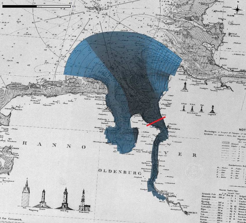
J. Mar. Sci. Eng. 2021, 9, 448                                                                                               3 of 21

                                 Figure 1. The Weser Estuary divided into the Outer Weser the Lower Weser and the adjacent Jade
                                 Bay. The cities of Bremerhaven (BHV), Nordenhamm (NH), Brake (B) and Wilhelmshaven (WHV)
                                 are indicated on the map for reference. The small map (Open Street Map) gives the location of the
                                 Weser Estuary in the German Bight and the satellite image taken from Copernicus Sentinel-2 (ESA)
                                 shows the present channel and shoal pattern in the Outer Weser with the constructed training walls
                                 and groynes marked in yellow.

                                 2. Materials and Methods
                                 2.1. The Flat-Bed Approach
                                       Process-based flat-bed models have been widely applied for the production of channel
                                 and shoal patterns in tidal inlets and geometrically constrained estuaries [16,18,19,31]. This
                                 study differs from the previous ones in the sense that a wide estuary is modeled here and
                                 the applied model is steered by simplified boundary conditions.
                                       In the application of a schematized Delft3D model, special attention is paid to the ini-
                                 tiation of the model. For undisturbed natural morphological development, the influence of
                                 a discrete bathymetry needs to be minimized in order to allow unconstrained development.
                                 This is achieved by applying a flat bed as initial bathymetry [18,19]. The estuarine geometry
                                 is based on the available historical charts and kept fixed for the base case simulation.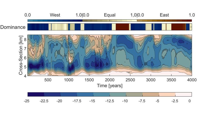
J. Mar. Sci. Eng. 2021, 9, 448                                                                                                  4 of 21

                                 2.2. Sediment Transport Formulation
                                      In this study, Delft3D [32] is applied. Delft3D is a process-based model, including
                                 the FLOW- (for hydrodynamics) and MOR- (for morphodynamics) modules, which are
                                 essential for this study. The Delft3D-FLOW module is based on the Reynolds-averaged
                                 Navier–Stokes equations under the assumption of incompressible fluids, shallow water
                                 and Boussinesq approximation. These are solved on a curvilinear/structured grid with
                                 an implicit finite-difference scheme (as default), as shown by [32] and described in the
                                 manual [33].
                                      Sediment transport is based on the Engelund–Hansen equation [34], which consid-
                                 ers the total transport load as bedload transport only and is a good approximation for
                                 transport of noncohesive sediments as shown by prior studies [13,18,35]. Additionally,
                                 Reyns et al. [36] showed that the Engelund–Hansen transport formula works well in com-
                                 bination with the so-called MorFac approach [11], which will be discussed later. The bed
                                 elevation is dynamically updated at each hydrodynamic time step.
                                      For bedload transport, bed slope effects can be considered by the factors αbs (in local
                                 flow direction) and αbn (normal to the local flow direction) as proposed by Bagnold [37] and
                                 Ikeda [38]. The bed slope factor in local flow direction αbs is kept constant with the default
                                 value of 1 due to its limited influence [39] and will be not discussed further. However,
                                 the additional normal transport vector as presented by van Rijn [40] is a sensitive tuning
                                 parameter, which has a considerable influence on the developing morphology [41]. It is
                                 defined as:
                                                                    ~Sb,n = |S′ |αbn ub,cr ∂zb                              (1)
                                                                              b
                                                                                     |~ub | ∂n
                                 with ~Sb,n being the additional transport vector calculated by Sb′ , the initial transport vector,
                                 αbn , the user-defined coefficient for calibration, ub,cr , the critical near-bed flow velocity, ~ub ,
                                 the near-bed flow velocity and ∂z    b
                                                                    ∂n , the bed slope normal to the flow direction.
                                        The additional transport vector resulting from the calibrated αbn value can compensate
                                 for artificially created steep slopes, too deep and narrow channels, which are caused by
                                 missing processes in the model formulations (e.g., avalanching mechanisms), simplified
                                 transport equations and potential numerical effects [42]. In particular, when simulating
                                 long-term morphodynamic development of channel and shoals in combination with mor-
                                 phological acceleration factors, as discussed later, the determination of the additional
                                 transport vector gains importance [18,43]. A detailed analysis of the function and effects of
                                 the slope factors is presented by Baar et al. [41]. By increasing αbn , the bedload transport
                                 normal to the local flow direction is increased, leading to a generally smoother channel
                                 pattern. Following this tendency, high αbn values might restrict realistic development of
                                 channels due to refilling from the channel banks. Therefore, αbn should be chosen and
                                 treated carefully.
                                        Additionally, as αbn only influences the bedload transport, it has a different order
                                 of magnitude for the Engelund–Hansen transport formula, with 100% of the transport
                                 considered as bedload, in comparison to the van Rijn transport formula, where only about
                                 10% of the transport is bedload [43]. For the Engelund–Hansen transport formula, applied
                                 in this study, a calibrated αbn value of 7.5 is used in all simulations.
                                        For the purpose of acceleration in the morphological development a morphological
                                 factor (MorFac) is used [11,12]. The MorFac accelerates morphological changes by multi-
                                 plying the erosion and deposition fluxes per computational time-step with a constant or
                                 time varying value [33]. To speed up morphological simulations, various techniques can
                                 be used, based on the difference in time scales between the hydrodynamics and the mor-
                                 phodynamic response [44]. Simplifications can be made by schematizing the tide [44] or by
                                 using ensemble techniques to model the tides [45]. These studies indicate that reducing the
                                 tidal signal to a single tidal constituent is not sufficient. We therefore apply multiple tidal
                                 constituents in this study. Here, we follow the approach of the morphological factor as
                                 proposed by Roelvink [11] and later on used in other studies as well, e.g., [16,18,19,35,42].
                                 In this approach, the bed level update per time step is multiplied by a factor, the so-called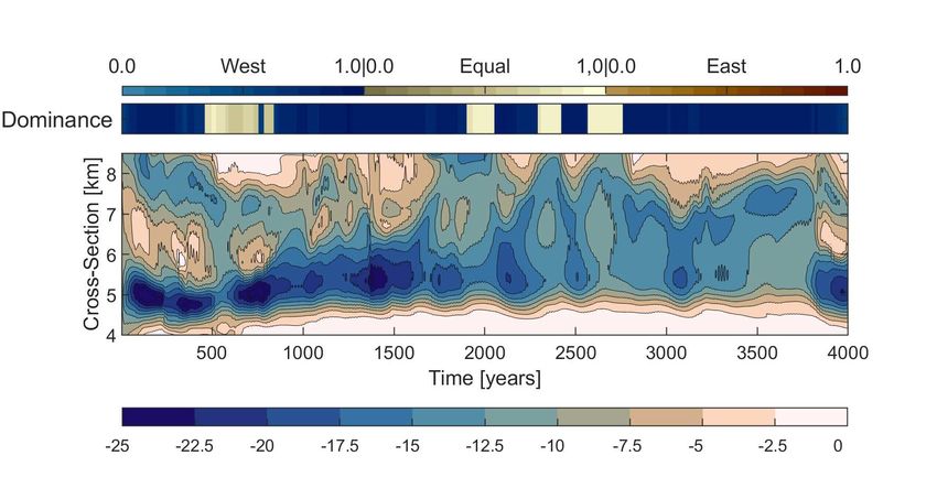
J. Mar. Sci. Eng. 2021, 9, 448                                                                                             5 of 21

                                 morphological factor. The approach is based on the assumption that the timing of the mor-
                                 phological change on intratidal scale is of minor importance. This implies that computing
                                 n times ebb flow and then n times flood flow results in the same morphology as computing
                                 n full tides (see Ranasinghe et al. [12] for a more detailed explanation).
                                      Studies have shown that, depending on the application, a MorFac of up to 1000 can be
                                 used to simulate long-term morphodynamic development [36]. The attempt for a critical
                                 MorFac definition [12,36] resulted in a formula, inspired by the Courant condition, that
                                 relates the propagation speed of bed forms to the available cell size. For applications similar
                                 to the present one, MorFacs of up to 300 and 400 are documented [16,18,19].
                                      Calculating a critical MorFac according to [36] leads to a critical MorFac in the order
                                 of 800, which is a high value in general. In this study, a MorFac of 400 is applied. In-
                                 creasing/decreasing the MorFac corresponds with increasing/decreasing the time step
                                 for morphological modeling. Therefore, this numerical parameter needs to be selected
                                 based on requirements: A valid MorFac has to be small enough to satisfy two requirements
                                 related to respectively stability and accuracy of the simulations.
                                      Regarding stability, MorFac values much larger than the chosen one may result into
                                 model instabilities meaning a violation of the stability criterion. The consequence of
                                 violating the stability requirement is that simulations cannot be carried out until the end.
                                 This can be an issue, especially with particular artificial initial conditions. An additional
                                 morphological stability criterion, the development of a morphological equilibrium, can be
                                 introduced. In this study, the morphological equilibrium is essential, in accordance with
                                 the investigation approach.
                                      Regarding the accuracy criterion, it needs to be ensured that a further decrease of the
                                 MorFac will not affect model results. This prevents using a MorFac that overestimates
                                 sediment transport, leading to deeper channels, more exposed flats and less intertidal area.
                                      The given MorFac value is applicable if the simulation is stable, a morphodynamic
                                 equilibrium develops and the resulting channel and shoal distribution does not vary
                                 significantly when applying smaller MorFacs. These aspects are analyzed by calculating
                                 the development of hypsometric curves of the model domain over time for the different
                                 MorFacs applied (50, 100, 200 and 400). Figure 2a presents the range of the resulting
                                 development of the hypsometric curves integrated over the model domain and plotted
                                 over time. Here, the same depth contour lines (indicated by the colors in Figure 2a are
                                 calculated in their cumulative percentage of appearance in the model domain (y-axis) for
                                 each of the MorFacs over time (x-axis). The span of the same contour lines between the
                                 different MorFacs is filled with the respective color (rather than the span of the depth range
                                 as typically seen). Additionally, the individual contour lines of the specific depths for the
                                 MorFac 400 are highlighted. The hypsometry starts with an unrealistic, artificial pattern,
                                 based on the uniform initial depth. During the MorFac simulations, each develops a
                                 channel and shoal pattern, changing the hypsometry in a similar way (small colored spans).
                                 At the end, a realistic distribution of the total area to different depth ranges is established,
                                 representing a realistic hypsometry. Figure 2b shows the individual hypsometric curves
                                 for the evaluated MorFacs after 2000 years of development as the cumulative percentage
                                 appearance (y-axis) of the developed depths (x-axis). The variations in the hypsometric
                                 development in Figure 2a are generally small with a local maximum of around 10%.
                                 Differences in the hypsometric curve at the end of the evaluation in Figure 2b are minimal.
                                 Hence, a decrease of the MorFac does not give different model results. Additionally,
                                 Figure 2a,b show a realistic hypsometry developed for all tested MorFacs. Thus, the
                                 accuracy requirements are fulfilled for the MorFac 400.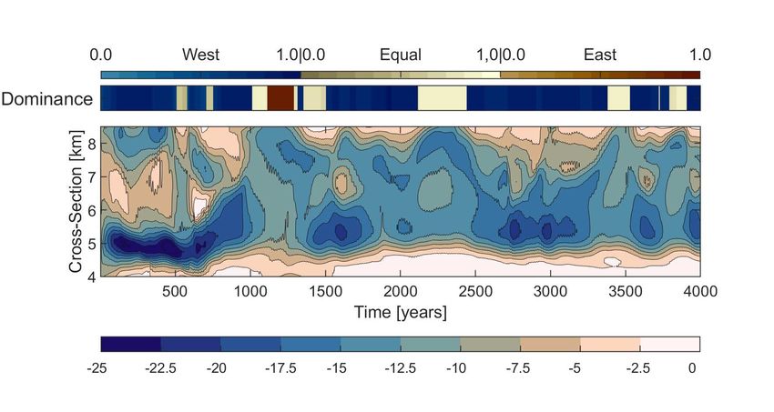
J. Mar. Sci. Eng. 2021, 9, 448                                                                                                6 of 21

(a)                                                                                        (b)

      Figure 2. Validation of the morphological factor by (a) the development of cumulative relative incident (in [%]) of depth
      contour lines as the colored span of contour lines from the MorFacs 400, 200, 100, 50 (MorFac 400 in thick) and (b) the
      individual hypsometric curves after 2000 years.

                                 2.3. Model Set-Up
                                      A curvilinear rectangular grid is generated covering the Jade-Weser estuary from
                                 Bremen-Vegesack to a few kilometers into the North Sea (see Figure 3). Model boundaries
                                 are aligned to the historical land boundaries, which resemble the overall shape of the
                                 present ones. The grid cell resolution varies from around 103 m in the most outer North
                                 Sea part and around 102 m in the inner part of the model domain. The latter resolution is
                                 present in the area of interest. Both resolutions are based on the length scales of the channel
                                 and shoal features that can be found in the Weser estuary historically and at present.
                                      The initial depth has a value of 7.34 m and is determined by the mean water depth of
                                 the Jade-Weser-area from a historical chart of the year 1878.
                                      The model is steered by two open boundaries: The tidal constituents O1, K1, M2, S2,
                                 M4, MS4 and M6 on the northern model domain side and a constant river discharge on
                                 the southern end. The amplitudes and phases of the tidal constituents along the open
                                 boundary are extracted from a larger model (Jade-Weser-Elbe-Model) maintained by the
                                 Federal Waterway Engineering and Research Institute [46]. It is assumed that this tidal
                                 signal is representative for the historical tidal regime, based on the findings of schematized
                                                                                        3
                                 model studies [18,31]. The river discharge is 325 ms in alignment with the yearly averaged
                                 fresh water discharge historically [30] and at present [3].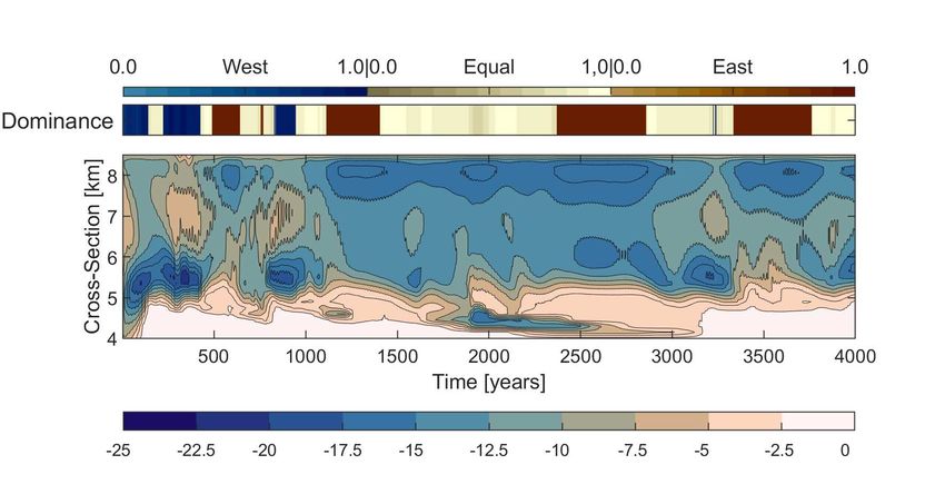
J. Mar. Sci. Eng. 2021, 9, 448                                                                                                       7 of 21

                                       Figure 3. Model domain and grid—created on the basis of historical maps—with a background map
                                       from 1862. The cross-section 75, which is essential for the results and discussed later, is marked
                                       in red.

                                            One noncohesive sediment fraction was used, as it was used in similar studies [18,19].
                                       A 200 µm sand is in good agreement with the dominating sediment fraction in the Outer
                                       Weser area based on the data available in Geopotenzial Deutsche Nordsee [47]. The
                                       available sediment thickness varies between 25 and 35 m and is limited by a non-erodible
                                       Holocene layer [47].

                                       2.4. Scenario Composition
                                            A classification of estuaries from Boyd et al. [48] considers three main influences
                                       that shape an estuary: tides, waves and river discharge. For the German Bight, Kösters
                                       and Winter [23] looked at different combinations of tides, wind stress and waves to in-
                                       vestigate resulting bottom shear stresses and morphodynamic changes. Furthermore,
                                       Herrling et al. [20] analyzed the effect of tides, wind-induced waves and currents as well
                                       as swells for the Outer Weser estuary. Their results suggest that the influence of wind
                                       stress and waves on the main channel morphodynamics can be neglected considering the
                                       schematization of this study. However, Herrling et al. [20] found that locally generated
                                       wind waves are influencing the morphodynamics of the inter- and supratidal area, which
                                       should be kept in mind, when looking at the results of this study. Nevertheless, these
                                       are not considered due to the anticipated spatial scale of this study and the simplified
                                       investigation approach. Therefore, five scenarios are defined (see Table 1).

      Table 1. Scenario Composition Synthesis: Listing of the scenarios selected for investigation on the left, based on the different
      aspects of the tides and river discharge that are potentially responsible for the formation of a two-channel system. The
      affiliation of the scenarios to either tides or discharge is indicated by the dots within the columns in the middle, followed by
      a description of the effects the scenario en- or disables, respectively.

            Scenario             Tides             Discharge       Description
  No Kelvin Wave                   ·                               No phase shift in the tidal constituents at the open boundary.
       No Coriolis                 ·                               No Coriolis effect included by setting the model latitude to zero.
   Increased Tides                 ·                               110% amplitude for tidal constituents (seasonal/long-term effects).
     No Discharge                                      ·                                        3
                                                                   A constant discharge of 0 ms at the southern open boundary.
  Max. Discharge                                       ·                                                  3
                                                                   A constantly high discharge of 2000 ms is defined.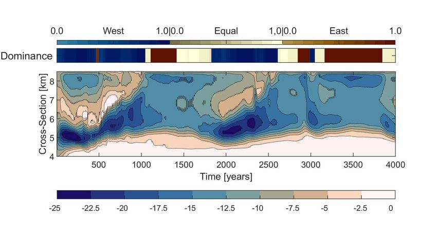
J. Mar. Sci. Eng. 2021, 9, 448                                                                                             8 of 21

                                      The funnel shape of the Weser estuary and previous studies [3,20,23] suggest that
                                 tides play the most important role in the morphodynamic development of the shoals and
                                 channels. Hence, special attention is paid to the tides. Two parts of the tides potentially
                                 influence the development of two-channel systems. The first part is the strength of the
                                 tides as such or relative to the river discharge. Variations in the tidal amplitude, based
                                 on seasonal or long-term effects, could lead to multiple conditions that are present for a
                                 limited time and individually support a western or an eastern channel in the Outer Weser
                                 Estuary, respectively. If each condition stabilizes a channel one site, the two-channel system
                                 could be based on two alternating tidal conditions (tidal range). Thus, by comparing
                                 a scenario simulation with a 10% increased tidal amplitude to the simulation with 0%
                                 increase (base case), it can be revealed if this hypothesis is true for the Outer Weser Estuary.
                                 Second, the spatial appearance based on deflections of the tides inside the estuary can
                                 lead to more pronounced channels on different sides of the estuary. Two main deflections
                                 are considered here: the Kelvin wave and the Coriolis effect. The latter deflects flows to
                                 the right, as the Weser Estuary is located at 53◦ north. The Kelvin wave is a result of this
                                 Coriolis-based deflection in the North Sea basin where a circular tidal wave propagation
                                 forms [49]. It causes a phase shift of the tidal wave in the German Bight, and thus at the
                                 offshore boundary of the Outer Weser. Both deflections might influence the location of a
                                 more dominant channel by pushing the ebb flow, flood flow or river discharge toward one
                                 side of the estuarine land boundaries. Consequently, a simulation without the Coriolis
                                 effect and one without the phase shift at the open boundary should reveal their effects
                                 on the two-channel system, respectively, when comparing their results to the base case
                                 simulation results, where both influences are included.
                                      Additionally, two extreme river discharge cases are added to the scenario list.
                                      The listed effects will be investigated in a three-step routine. First, the model setup is
                                 adapted such that the effect is included or not included. Second, a simulation is run. Third,
                                 the results of the scenario simulation are compared to the base case simulation, revealing
                                 the influence of the selected scenario on the channel and shoal development.

                                 2.5. Postprocessing Methods
                                      The development of the two-channel system and the corresponding morphological
                                 state is investigated by analyzing the temporal development of a cross-section regarding
                                 the dominance of western, eastern or middle channels. A novel method is to quantify
                                 the dominance of certain channel–shoal patterns in cross-sections (correlation analysis of
                                 (cross-)section evolution—CASE method). A small number (n) of cross-section types is de-
                                 termined from the baseline simulation (Figure 4a, with three exemplary cases) representing
                                 distinctive channel–shoal patterns with a certain feature, or a certain type of channel–shoal
                                 pattern. Each distinctive cross-section type defines a case, resulting in n cases that can
                                 optionally be organized in groups of equal channel–shoal pattern types (Figure 4b, with
                                 (blue = western dominance, yellow = equal dominance and red = eastern dominance)). All
                                 available cross-sections from different scenarios and/or different points in time are then
                                 correlated to these cases (schematized in Figure 4c), leading to n correlation coefficients
                                 between −1 and 1 for each point in time (Figure 4d). Based on the cross-section type with
                                 the maximum correlation, the dominant channel–shoal pattern is determined (Figure 4e).
                                 The degree of resemblance is further indicated by the correlation value (e.g., visualized
                                 by color intensity). This method is applied here to an exemplary cross-section, which lies
                                 within the center of the area in which the two channels occur (see Figure 3). From the base
                                 case scenario simulation, nine cross-section types are chosen (see Figure 4). Each of the nine
                                 cross-section corresponds to a morphological state of western channel dominance, equal
                                 channel dominance or eastern channel dominance (3 types each category). The base case is
                                 used for the definition of the cases due to its comparability with the scenario simulations.
                                 With this method, a time series of cross-sections is translated to a time series of dominance
                                 types for each scenario.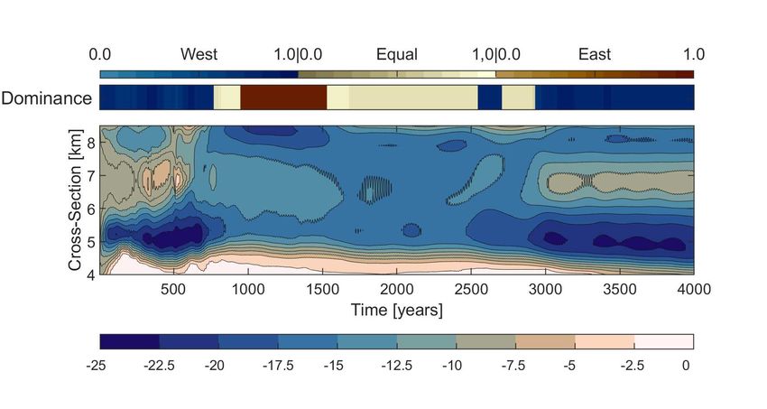
J. Mar. Sci. Eng. 2021, 9, 448                                                                                                       9 of 21

      Figure 4. Graphical description of the CASE method with (a) the selection of representative cases, (b) the final nine cases
      for this study, (c) the correlation analysis over time, (d) the resulting correlation values and (e) the final result, where the
      morphological state is presented over time with the corresponding case (color) and its correlation value (color intensity).

                                        To visually compare the temporal development of the two-channel system in the dif-
                                   ferent scenarios, Hovmöller diagrams [50] are used which display the cross-section depths
                                   over time. Above each of those diagrams, a bar plot indicating the dominant two-channel
                                   type and the strength of the correlation calculated with the CASE method is displayed. The
                                   channel dominance categories are visualized by different colors (green for western, red for
                                   eastern and light yellow for equal dominance). Additionally, by showing the corresponding
                                   cross-correlation values through color intensity, plausibility of the respective category is
                                   indicated. With this approach of combining Hovmöller plots with results of the CASE
                                   method, a visual inspection of the temporal development of each scenario is combined
                                   with a quantitative classification of the corresponding morphological states.

                                   3. Results
                                   3.1. Base Case
                                        The results of the base case simulation show a good representation in the Outer Weser
                                   estuary. A two-channel system clearly develops (see Figure 5) and remains morphody-
                                   namically active. The locations and depths of the channel are reasonable compared to
                                   naval charts. For the base case simulation, the criteria for morphodynamic equilibrium are
                                   reached after 650 years (the product of the hydrodynamic time and the MorFac) according
                                   to Figure 6. The results in Figure 6 are based on the hypsometric development of the
                                   area of interest (visualized in Figure 5b–f) and the cumulative bedload transport of the
                                   representative cross-section (indicated in Figure 3). Thus, for the base case, the first two
                                   research questions stated in the introduction can be confirmed.
J. Mar. Sci. Eng. 2021, 9, 448 10 of 21
(a) Channel area from hist. charts (b) After 650 years (c) After 900 years
(d) After 2000 years (e) After 3200 years (f) After 4000 years
Figure 5. Simulation results of the base case. In (a), the locations of the tidal channel system from three historical charts
(1812, 1859, 1870) are intersected. In (b–f), results of the morphological simulations are shown for different years, with
channel depths in blue and shoals in earth colors.
The equilibrium point is shown in Figure 5b, where a number of side channels exist
in addition to the two main channels. Afterward, the established two-channel system
remains morphodynamically active and switches between two clearly separated channels
(Figure 5c,e) and two almost unified channels (Figure 5d,f). Furthermore, an alternation
of the location of the deepest channel can be found in the results, which connects to the
third research question. Figure 7 visualizes the alternation applying the CASE method.
Looking at the reversed Hovmöller diagram, the western channel is more prominent.
Additionally, a channel and shoal scheme is present repetitively. First, a deep and wide
channel develops on the western side (beginning–1200 years, 1850–2600 years and 3000–
3100 years), followed by the development of an eastern channel (1250–1700 years, 2800–
2950 years and 3200–3800 years), which becomes more dominant as the western channel
becomes shallower at the same time. With respect to the third research question, there is a
more dominant channel and even an alternation of the latter is found. This is approved
by the correlation analysis (top of Figure 7), where the recurrent pattern of the prevailing
western dominance (green) and eastern dominance (red) is illustrated. Additionally, there
are periods where neither of the channels is more dominant (yellow). Overall, correlation
values are high (>0.75) after initiation.J. Mar. Sci. Eng. 2021, 9, 448 11 of 21
Figure 6. Development of the hypsometry over time in the area of interest (left y-axis) combined with the cumulative
bedload transport over time (right y-axis). Both trajectories tend to become linear over time which is considered to prove
morphodynamic equilibrium.
Figure 7. Depth of the investigated cross-section over time, showing the alternation of the two-channel system. The channel
dominance calculated by the CASE method is displayed above, greenish colors indicating western dominance, reddish
colors indicating eastern dominance and brownish indicating a balanced two-channel system, the shading within each color
indicating the strength of the correlation.
As all research questions are answered positively, the influences of the predefined
forcings (Section 2.4) are investigated.
3.2. Effects of Varying Tide
The effects of the tidal scenarios are presented according to the research questions
and results are summarized by applying the CASE method (Figure 8). For the bathymetric
development of the scenarios, see the Appendix A.
First, all three scenarios reach a morphological equilibrium and show a clear two-
channel system developing (Figure 8). Comparing the two-channel systems developing in
the tidal scenarios with the base case reveals similarities with respect to the general two-
channel system and the formation and variation of deeper channels. However, comparingJ. Mar. Sci. Eng. 2021, 9, 448 12 of 21
the location and dynamic alternation of the deepest channel to the base case results shows
considerable variations. In a nutshell, the first two research questions are answered posi-
tively and by elaborating on the third question differences can be identified more clearly.
(a) Discard of the Kelvin wave at the open boundary.
(b) Neglecting the Coriolis effect within the model domain.
(c) Increased tidal range by 10% for each component.
Figure 8. Two-channel system alternation for the tidal scenario simulations (description, see Figure 7).
Starting with the location of the deepest channel, the no Kelvin wave scenario shows
a more distinct western channel (Figure 8a). The opposite holds true for the no Coriolis
scenario (Figure 8b). Additionally, a mixed development is seen in the increased tidal
range scenario (Figure 8b): Although the deeper channel can be found on the western side
most of the time, the channel and domination pattern is more mixed compared to the other
scenarios. Next, the dynamics of the domination pattern are found: In the no Kelvin wave
scenario, an almost regular alternation is established, mainly between western and equal
dominance (Figure 8a). An alternation period of 500–1000 years is shown. The absence
of the Coriolis effect leads to a more stable eastern channel and less frequent alternationsJ. Mar. Sci. Eng. 2021, 9, 448 13 of 21
between eastern and equal dominance (Figure 8b). Lastly, an increased tidal forcing creates
a more frequent and expansive alternation (Figure 8c). Especially between 1500–2650 years
and after, a complete shift of the dominance from west to east develops.
3.3. Effects of Varying Discharge
Similar to the tidal scenarios, the river discharge scenarios both reach a morphological
equilibrium and show a two-channel system (Figure 9). However, with respect to the base
case, the results of the two simulation reveal significant differences. For the scenario with-
out any discharge (Figure 9a), periodically, a two-channel system develops and disappears
when only one channel is present only. This is the western channel for the majority of the
simulation period. The scenario with extreme discharge (Figure 9b) reveals a two-channel
system that almost unifies into one large channel for a limited period but then divides into
two clear channels.
(a) No discharge from the Weser river.
(b) Extreme river discharge of 2000 m3 /s
Figure 9. Alternation of the two-channel system for the river discharge scenario simulations (description, see Figure 7).
Accordingly, the alternation is relatively slow for both cases, especially for the extreme
discharge scenario. Here, the CASE method indicates that there is one full alternation
of channel dominance only in 4000 years. The cross-sectional plot supports this finding
as described previously. In the no discharge scenario, some alternating features can be
found even though the dominance does not fully alternate. Additionally, due to general
orientation of the channels toward the west in combination with the established channel
on the western side, a clear alternation is seen from 1750 to 3000 years. This observation is
supported by the recurrent pattern in the cross-correlation revealed by the CASE method.J. Mar. Sci. Eng. 2021, 9, 448 14 of 21
3.4. Synthesis
Figure 10 shows the CASE method results for all scenarios, indicating the influence of
the forcing on the two-channel system. Two aspects are included in Figure 10 for each sim-
ulation: first, the individual distribution of channel dominance in the two-channel system,
and second, the resulting alternation activity (counts of changes between morphological
states). The alternation activity is not necessarily referred to full alternations from western
to eastern dominance and back. By comparing both aspects for the scenarios with the
base case, conclusions can be drawn about the increase or decrease of either channel or
alternation presence.
BC no KW no CO +TR no Q +++Q
100 30
90
Percentage of Morphological States
25
80
70
Alternation Counts
20
60
50 15
40
10
30
20
5
10
0 0
West Equal East Alternations
Figure 10. Comparison of the occurrence of channel dominance distribution (%) per scenario. With
BC = base case, no KW = no Kelvin wave, no CO = no Coriolis effect, +TR = increased tidal range, no
Q = no river discharge and +++Q = extreme river discharge. The number of alternations (changes
between morphological states) is shown by the blue diamonds.
An enhanced eastern channel can be found when the influence of the Kelvin wave
and the mean river discharge are included (as no Kelvin wave or no discharge show less or
no percentage of eastern channel dominance). Thus, both influences have the potential to
significantly increase the presence of eastern channel dominance. The opposite holds true
for the effects of Coriolis (when Coriolis is actually included like it is in the base case), an
increased tidal range and extreme river discharge, as indicated by the higher percentage of
the green bars in Figure 10. Hence, the western channel is supported by these three effects.
The enhancement of one of the two channels correlates with a decreased alternation
activity. The base case, where Coriolis and the Kelvin wave are included, has a lower
alternation count compared to the simulations, where these effects are disabled. Extreme
river discharge leads to even less changes in the morphological state as for the base case.
Higher alternation activity is found with an increased tidal range and with mean river
discharge (no river discharge compared to the mean discharge of the base case). However,
the increase in alternation activity of the increased tidal range is considerably higher,
compared to the mean river discharge. These findings will be discussed below.J. Mar. Sci. Eng. 2021, 9, 448 15 of 21
4. Discussion
The base case simulation shows the development of a two-channel system and its
morphodynamic activity over a period of 4000 years. Within a period of 650 years, a
morphodynamic equilibrium is established and remains at its state from that point onward.
Both aspects, the development of a two-channel system and reaching morphodynamic equi-
librium, imply a successful application of the modeling approach described in Section 2.1.
A comparison with nautical charts (from the time before human interventions changed
the morphology of the Weser estuary) reveals that the extent and the migration area of
the individual channels is plausible. However, the exact location and dimensions of the
individual channels differ to some degree from the observed ones, which is presumably
caused by the simplicity of the modeling approach. A key disparity is that the channels
generally tend to become too deep in comparison with documented bathymetries, which
is a known issue for Delft3D models as discussed by [42]. Nevertheless, the reasonable
results of the base case allow the execution of the designed scenarios.
Here, the variety of developed two-channel systems offers valuable insight into the
impact of several parameters on morphodynamic development. The synthesis of all
scenario results in the conclusion that the development of the two-channel system is
mainly caused by the relation of tides and river discharge in combination with the basin
geometry. This is in alignment with the hypothesis given in Section 2.4. The relation of
tides and discharge can be interpreted as the tides being the main driver and decisive for
the formation of the channels. A strong indicator for this reasoning is the result of the no
river discharge scenario, where a two-channel system is found based on the tidal forcing
only. Due to the absence of river discharge, the western channel establishes stronger than
the eastern channel as indicated by the CASE method in Figure 9a.
Thus, in order to get a two-channel system with equally deep channels, it takes a
combination of tides and river discharge. The results of the increased tidal range scenario
and extreme discharge verify this finding (Figure 10 and Figure A2). The results of the
various scenarios reveal a trend: the more tides are dominating over discharge (+ tidal
range, Figure 10), the more a western channel develops, while more discharge favors
the development of an eastern channel. However, this only applies as long as Coriolis is
included, causing a reflection of the incoming tidal wave to the right. This holds true for
the extreme discharge scenario as well; however, it can neither be seen in Figure 10 nor in
the CASE method results. The reason is that the extreme discharge scenario creates a stable
two-channel system, where the eastern channel becomes dominant further offshore of the
selected cross-section (see Figure A2e,f), and is thus not covered by the CASE method.
The dependence of the well-established western channel on the Coriolis effect implies
that the flood flow is deflected to the western side and the ebb flow to the eastern side,
causing the two-channel system with a flood channel in the west and an ebb channel in
the east. The results of the scenario simulation neglecting the Coriolis effect, where the
eastern channel is more pronounced, would support this reasoning. Additionally, the
comparison between the no discharge scenario and the base case simulation (with average
discharge) agrees with the latter observations, as the consequently larger magnitude of
offshore directed flow (deflected to the eastern side by the Coriolis effect) results in a
stronger eastern channel. Following this reasoning, the no discharge scenario shows that
ebb flow alone is strong enough to create the eastern channel. However, the depth averaged
velocities calculated in the two channels do not support the argumentation of a flood and
ebb channel, as their magnitudes are almost identical (J. Mar. Sci. Eng. 2021, 9, 448 16 of 21
enhanced western channel. This behavior is reasonable as the incoming tides approach the
east side of the Outer Weser due to the northwestern-originated Kelvin-wave-based inertia.
Although validation of the scenario simulations remains challenging due to their
conceptualized character, the justification criteria applied for the base case holds true for
the scenario simulations as well. All simulations reach a morphodynamic equilibrium
and the developed morphology is reasonable, although channels tend to be too deep.
The influence of the basin geometry is not part of this research but raises interesting
research questions.
Another remarkable finding is a variety of alternation patterns (Figures 7–9) and
periods (Figure 10). These depend on the domination of the tides (with respect to river
discharge) and the depth of the channels. The first aspect is shown by the trend in Figure 10,
where an increased tidal range increases alternation, followed by mean river discharge,
which increases alternation based on the domination of tides and the more equally es-
tablished two-channel system. If the tidal flow is overruled by extreme river discharge,
alternation is reduced. Additionally, if one channel is more pronounced, it takes more time
to alter as seen for the Kelvin wave and Coriolis effect. As fascinating as the alternation
results are, a justified quantification remains challenging, almost impossible for two rea-
sons. First, as mentioned earlier, the channel depth is overestimated in all simulations. As
this is relevant for the alternation period, the resulting alternation periods are probably
overestimated as well. Second, the alternation dynamics shown in Figure 10 are based on
the CASE method with one cross-section analyzed, leading to a local observation. Addi-
tionally, by selecting the representative cases from the base case simulation for the CASE
method, the channel and shoal patterns are simplified and therefore less accurate, despite
high cross-correlation values.
In reports, alternation periods have been described varying between 20 and
120 years [4,28,30]. Compared to the time span of an alternation in Figures 7–9, these
are rather short periods, whereas the simulated alternation periods are up to ten times
longer. Thus, a comprehensive analysis of the causes and reasons for the alternation does
not seem to be feasible with the modeling approach chosen.
To put our results into perspective, we compared them with results from similar
studies of other systems. Two studies on the Western Scheldt Estuary, Netherlands [18,19]
and one on the Qiangtangjiang Estuary, China [51] are considered. The comparison shows
similarities, but it also reveals the importance of accounting for the specific signatures of
each study site. Similarities are found in the development of a morphological equilibrium
and the dependence of the locations of channel and shoals on the estuarine geometry. The
studies at both systems indicate a strong influence of the basin geometry on the results of
the large scale tidal channel and/or bar developments. Furthermore, Dam et al. [19] and
Yu et al. [51] found that a morphological equilibrium is reached in both estuaries. Moreover,
the estimated time span for reaching a morphological equilibrium has a comparable order
of magnitude as the time spans determined in this study.
Partly similar results are found for the influence of river discharge on the model
result. For the Qiangtangjiang Estuary [51], it was found that a channel and shoal pattern
develops, even if no discharge is imposed. This is in agreement with the results shown in
Section 3.3. Nevertheless, a dependence of the offshore shoal extent on the river discharge
as indicated by Yu et al. [51] cannot be identified in this study. However, the average
discharge in the Qiangtangjiang Estuary is an order of magnitude larger compared to the
Weser Estuary and the investigation of Yu et al. [51] is more schematized (an idealized
funnel shape). In the Western Scheldt Estuary [18], river discharge affects the development
of the channel and shoal system in a way similar to that in our study. However, van der
Wegen and Roelvink [18] found that an extreme river discharge enhances the ebb channel,
unlike in this study, where there is still a two-channel system at almost the same location
as for normal or no river discharge. The explanation for this difference could be the more
restricted geometry of the Western Scheldt. Additionally, the deviation in ebb and flood
channels is not applicable for the results in this study as discussed before.J. Mar. Sci. Eng. 2021, 9, 448 17 of 21
The alternation of a more dominant channel within a two-channel system appears
to be unique for the Weser Estuary and has not been detected or described in any of the
previous studies. Furthermore, the influence of the Coriolis effect, the Kelvin wave and an
increased tidal range has not been investigated by one of the three other studies [18,19,51].
The flat bed approach in combination with a high MorFac and simplified boundary
conditions is a handy method to investigate large-scale morphodynamic features and
developments with reasonable accuracy and computational effort. However, there remains
some potential for optimization, which may be addressed in future research. A point
that could not be improved during this research is the development of the tidal range
inside the Lower Weser. While the tidal range in the area of interest meets the documented
historical tidal range, the tidal range becomes too high when traveling inside the estuary
compared to historical measurements. The cause for the amplified tidal range lies in the
flat bed modeling approach, as there is not enough friction in the Lower Weser to damp
the tidal wave during its propagation. As this is the case from the beginning, the narrow
and shallow channels that are necessary to generate the needed friction cannot develop
and the Lower Weser channel remains deep. An option to overcome this problem could
be introducing a gradient to the initial bathymetry, but it is not possible with the same
initial depth in the whole model domain. Another option mentioned in publications using
the flat bed approach is the consideration of non-erodible layers [18]. As described earlier,
these were applied in this study as well, but at the time, data were only available for the
outer part of the model domain, and thus not available for possible model improvements
in the Lower Weser.
Here, it needs to be mentioned that the analyses of the CASE method are based on
one cross-section within the area of interest that has been selected as representative.
5. Conclusions
This research presents how the channel development on the Outer Weser estuary
is influenced by tidal range, Coriolis effect, Kelvin wave and river discharge, based on
a novel analysis of schematized long-term morphodynamic simulations. Starting with
a flat bed, a morphodynamic equilibrium with a two-channel system is reached in all
simulations. Differences in the developing channel and shoal patterns show that each
forcing contributes more to one of the two channels than to the other. However, the
two-channel system is developing as a result of the tides in combination with the basin
geometry, as none of the investigated effects result in an only one-channel system, only. A
classification into a flood and an ebb channel is not supported by the results. Alternation
of the more dominant channel is found in the simulations, but assigning the responsible
forcing remains challenging. However, it is likely that this is a result of the interaction
between the tides and the basin geometry, as alternation periods are not linked to artificial
time scales of the model.
Simulation results are analyzed using the correlation analysis of (cross-)section evo-
lution (CASE) method developed in this study. It compares simulation results based on
cross-section correlation and presents the morphological state over time for each simulation.
The developed CASE method complements available methods for analyzing long-term
channel and shoal development but should be seen as a local indicator. It might provide
additional insight to further develop the CASE method to include more cross-sections.
Additionally, the cases selected in the base case simulation for the correlation analysis are
chosen manually and further criteria for their selection might improve the method.
Author Contributions: Conceptualization, J.G. and A.Z.; data acquisition, model setup, investigation
and writing—original draft, J.G.; data acquisition, supervision and writing—editing and reviewing,
A.Z., B.C.v.P. and Z.B.W. All authors have read and agreed to the published version of the manuscript.
Funding: The publication of this article was funded by the Open Access Fund of the Leibniz
Universität Hannover.J. Mar. Sci. Eng. 2021, 9, 448 18 of 21
Acknowledgments: This study was supported by the infrastructure of BAW. The authors want to
thank for the support and comments provided by the colleagues at BAW. All figures are processed
and prepared in Matlab and all color maps are taken from the scientific color maps of F. Crameri [52].
Furthermore, the authors thankfully gained ideas and supportive comments during the investigation
from Sierd de Vries and feedback on the manuscript by Jan Tiede, Leon Scheiber, Christian Jordan
and Zoë Vercelli.
Conflicts of Interest: The authors declare no conflict of interest.
Abbreviations
The following abbreviations are used in this manuscript:
BAW Federal Waterways Engineering and Research Institute
DOAJ Directory of open access journals
MDPI Multidisciplinary Digital Publishing Institute
MORFAC Morphological Factor
CASE Correlation Analysis of (cross-)Section Evolution
Appendix A. Scenario Results
Appendix A.1. Tidal Scenarios
No Kelvin Wave
(a) After 650 years (b) After 2600 years (c) After 4000 years
No Coriolis
(d) After 900 years (e) After 2600 years (f) After 4000 years
Figure A1. Cont.J. Mar. Sci. Eng. 2021, 9, 448 19 of 21
Increased Tidal Range
(g) After 1200 years (h) After 2600 years (i) After 4000 years
Figure A1. Results of the tidal scenario simulations at three different times in years (hydrodynamic
time times the morphological factor). The first time-step is selected based on equilibrium conditions.
Clear distinction between the channel (blue colors) and shoal (earth colors).
Appendix A.2. River Discharge Scenarios
No River Discharge
(a) After 900 years (b) After 2600 years (c) After 4000 years
Extreme River Discharge
(d) After 1200 years (e) After 2600 years (f) After 4000 years
Figure A2. Results of the river discharge scenario simulations at three different times in years
(hydrodynamic time multiplied with the morphological factor). The first shown time-step is selected
based on equilibrium conditions. Clear distinction between the channel (blue colors) and shoal (earth
colors) area.J. Mar. Sci. Eng. 2021, 9, 448 20 of 21
References
1. Vorwig, W.; Wiemann, U.; Kobbe, W. Seeschifffahrt und Häfen in Norddeutschland. In Statistische Monatshefte Niedersachsen;
11/2014; Landesamt für Statistik Niedersachsen (LSN): Hanover, Germany, 2014 .
2. Plate, L. Die Weser als Seewasserstrasse: Bilanzbericht, Bericht f. d. Küsten-Ausschuß, 1951.
3. Lange, D. The weser estuary: Heide, Holstein: Boyens. Die Küste 2008, 74, 275–287.
4. Göhren, H. Beitrag zur Morphologie der Jade-und Wesermündung. Die Küste 1965, 13, 140–146.
5. Wetzel, V. Der Ausbau des Weserfahrwassers von 1921 bis heute. In Jahrbuch der Hafenbautechnischen Gesellschaft; Springer:
Heidelberg, Germany, 1988; Volume 42, pp. 83–105.
6. De Swart, H.E.; Zimmerman, J. Morphodynamics of Tidal Inlet Systems. Annu. Rev. Fluid Mech. 2009, 41, 203–229,
doi:10.1146/annurev.fluid.010908.165159.
7. Roelvink, J.A.; Reniers, A.J.H.M. A Guide to Modeling Coastal Morphology; World Scientific: Hackensack, NJ, USA; London,
UK, 2012.
8. Friedrichs, C.T. Barotropic tides in channelized estuaries. In Contemporary Issues in Estuarine Physics; Cambridge University Press:
Cambridge, UK, 2010; pp. 27–61.
9. Van Veen, J. Ebb and flood channel systems in the netherlands tidal waters 1. J. Coast. Res. 2005, 216, 1107–1120, doi:10.2112/04-
0394.1.
10. Marciano, R.; Wang, Z.B.; Hibma, A.; de Vriend, H.J.; Defina, A. Modeling of channel patterns in short tidal basins. J. Geophys. Res.
2005, 110, 1155, doi:10.1029/2003JF000092.
11. Roelvink, J.A. Coastal morphodynamic evolution techniques. Coast. Eng. 2006, 53, 277–287, doi:10.1016/j.coastaleng.2005.10.015.
12. Ranasinghe, R.; Swinkels, C.; Luijendijk, A.; Roelvink, D.; Bosboom, J.; Stive, M.; Walstra, D. Morphodynamic upscaling with the
MORFAC approach: Dependencies and sensitivities. Coast. Eng. 2011, 58, 806–811, doi:10.1016/j.coastaleng.2011.03.010.
13. Van Maanen, B.; Coco, G.; Bryan, K.R. Modelling the effects of tidal range and initial bathymetry on the morphological evolution
of tidal embayments. Geomorphology 2013, 191, 23–34, doi:10.1016/j.geomorph.2013.02.023.
14. Nabi, M.; de Vriend, H.J.; Mosselman, E.; Sloff, C.J.; Shimizu, Y. Detailed simulation of morphodynamics: 2. Sediment pickup,
transport, and deposition. Water Resour. Res. 2013, 49, 4775–4791, doi:10.1002/wrcr.20303.
15. De Vriend, H.J.; Capobianco, M.; Chesher, T.; de Swart, H.E.; Latteux, B.; Stive, M. Approaches to long-term modelling of coastal
morphology: A review. Coast. Eng. 1993, 21, 225–269, doi:10.1016/0378-3839(93)90051-9.
16. Dastgheib, A.; Roelvink, J.A.; Wang, Z.B. Long-term process-based morphological modeling of the Marsdiep Tidal Basin.
Mar. Geol. 2008, 256, 90–100, doi:10.1016/j.margeo.2008.10.003.
17. Zhang, W.; Schneider, R.; Harff, J. A multi-scale hybrid long-term morphodynamic model for wave-dominated coasts.
Geomorphology 2012, 149–150, 49–61, doi:10.1016/j.geomorph.2012.01.019.
18. Van der Wegen, M.; Roelvink, J.A. Reproduction of estuarine bathymetry by means of a process-based model: Western Scheldt
case study, the Netherlands. Geomorphology 2012, 179, 152–167, doi:10.1016/j.geomorph.2012.08.007.
19. Dam, G.; van der Wegen, M.; Labeur, R.J.; Roelvink, D. Modeling centuries of estuarine morphodynamics in the Western Scheldt
estuary. Geophys. Res. Lett. 2016, 43, 3839–3847, doi:10.1002/2015GL066725.
20. Herrling, G.; Benninghoff, M.; Zorndt, A.; Winter, C. Drivers of channel-shoal morphodynamics at the Outer Weser estuary.
In Proceedings of the 8th International Conference on Coastal Dynamics, Helsingoer, Denmark, 12–16 June 2017.
21. Hesse, R. Zur Modellierung des Transports kohäsiver Sedimente am Beispiel des Weserästuars. Ph.D. Thesis, Technische
Universität Hamburg, Hamburg, Germany, 2020.
22. Lojek, O. Sensitivity Analysis of Single Storm Surges in the Jade-Weser Estuary. Ph.D. Thesis, Institutionelles Repositorium der
Leibniz Universität Hannover, Hannover, Germany, 2020.
23. Kösters, F.; Winter, C. Exploring German Bight coastal morphodynamics based on modelled bed shear stress. Geo-Mar. Lett. 2014,
34, 21–36, doi:10.1007/s00367-013-0346-y.
24. Casulli, V.; Walters, R.A. An unstructured grid, three-dimensional model based on the shallow water equations. Int. J. Numer.
Methods Fluids 2000, 32, 331–348.
25. Luan, H.L.; Ding, P.X.; Wang, Z.B.; Ge, J.Z. Process-based morphodynamic modeling of the Yangtze Estuary at a decadal timescale:
Controls on estuarine evolution and future trends. Geomorphology 2017, 290, 347–364, doi:10.1016/j.geomorph.2017.04.016.
26. Laurer, W.; Naumann, M.; Zeiler, M. Erstellung der Karte zur Sedimentverteilung auf dem Meeresboden in der deutschen
Nordsee nach der Klassifikation von FIGGE (1981). Geopotenzial Dtsch. Nordsee Modul B Dok. 2014, 1, 1–19.
27. Vos, P.C.; Knol, E. Holocene landscape reconstruction of the Wadden Sea area between Marsdiep and Weser. Neth. J. Geosci. 2015,
94, 157–183, doi:10.1017/njg.2015.4.
28. Ramacher, H. Der Ausbau von Unter-und Außenweser. In Mitteilungen des Franzius Instituts; TU Hannover: Hanover, Germany,
1974; Volume 41.
29. BfG. Sedimentmanagementkonzept Tideweser: Untersuchung im Auftrag der WSÄ Bremen und Bremerhaven; BfG: Koblenz,
Germany, 2014.
30. Plate, L. Forschungen als Grundlage für den Ausbau der Aussenweser. Dtsch. Wasserwirtsch. 1935, 4, 66–74.
31. Wang, Z.B.; Louters, T.; de Vriend, H.J. Morphodynamic modelling for a tidal inlet in the Wadden Sea. Mar. Geol. 1995,
126, 289–300, doi:10.1016/0025-3227(95)00083-B.You can also read