IGAPS images database - High resolution Hα imaging of the Northern Galactic Plane
←
→
Page content transcription
If your browser does not render page correctly, please read the page content below
Astronomy & Astrophysics manuscript no. main                                                                                        ©ESO 2021
                                               August 4, 2021

                                               High resolution Hα imaging of the Northern Galactic Plane, and the
                                                                    IGAPS images database
                                                R. Greimel1 , J. E. Drew2, 3 , M. Monguió2, 4, 5 , R. P. Ashley6 , G. Barentsen2, 7 , J. Eislöffel8 , A. Mampaso9 , R. A. H.
                                                Morris10 , T. Naylor11 , C. Roe2 , L. Sabin12 , B. Stecklum8 , N. J. Wright13 , P. J. Groot14, 15, 16, 17 , M. J. Irwin18 , M. J.
                                               Barlow3 , C. Fariña6, 9 , A. Fernández-Martín9, 19 , Q. A. Parker20, 21 , S. Phillipps10 , S. Scaringi22 , and A. A. Zijlstra23 ,21

                                                      1
                                                          IGAM, Institute of Physics, University of Graz, Universitätsplatz 5/II, 8010 Graz, Austria
                                                      2
                                                          School of Physics, Astronomy & Mathematics, University of Hertfordshire, Hatfield AL10 9AB, UK
                                                      3
                                                          Department of Physics & Astronomy, University College London, Gower Street, London WC1E 6BT, UK
                                                      4
                                                          Institut d’Estudis Espacials de Catalunya, Universitat de Barcelona (ICC-UB), Martí i Franquès 1, E-08028 Barcelona, Spain
arXiv:2107.12897v1 [astro-ph.GA] 27 Jul 2021

                                                      5
                                                          Universitat Politècnica de Catalunya, Departament de Física, c/Esteve Terrades 5, 08860 Castelldefels, Spain
                                                      6
                                                          Isaac Newton Group, Apartado de correos 321, E-38700 Santa Cruz de La Palma, Canary Islands, Spain
                                                      7
                                                          Bay Area Environmental Research Institute, P.O. Box 25, Moffett Field, CA 94035, USA
                                                      8
                                                          Thüringer Landessternwarte, Sternwarte 5, 07778 Tautenburg, Germany
                                                      9
                                                          Instituto de Astrofísica de Canarias, E-38205 La Laguna, Tenerife, Spain
                                                     10
                                                          Astrophysics Group, School of Physics, University of Bristol, Tyndall Av, Bristol, BS8 1TL, UK
                                                     11
                                                          School of Physics, University of Exeter, Exeter EX4 4QL, UK
                                                     12
                                                          Instituto de Astronomía, Universidad Nacional Autónoma de México (UNAM), AP 106, Ensenada 22800, BC, México
                                                     13
                                                          Astrophysics Group, Keele University, Keele, ST5 5BG, UK
                                                     14
                                                          Department of Astrophysics/IMAPP, Radboud University, P.O. Box 9010, 6500 GL Nijmegen, The Netherlands
                                                     15
                                                          Department of Astronomy, University of Cape Town, Private Bag X3, Rondebosch, 7701, South Africa
                                                     16
                                                          South African Astronomical Observatory, P.O. Box 9, Observatory, 7935, South Africa
                                                     17
                                                          The Inter-University Institute for Data Intensive Astronomy, University of Cape Town, Private Bag X3, Rondebosch, 7701, South
                                                          Africa
                                                     18
                                                          Institute of Astronomy, University of Cambridge, Madingley Road, Cambridge, CB3 0HA, UK
                                                     19
                                                          Centro Astronómico Hispano-Alemán, Observatorio de Calar Alto, Sierra de los Filabres s/n, E-04550 Gérgal, Almeria, Spain
                                                     20
                                                          The University of Hong Kong, Department of Physics, Hong Kong SAR, China
                                                     21
                                                          The Laboratory for Space Research, Cyberport 4, Hong Kong SAR, China
                                                     22
                                                          Department of Physics, University of Durham, South Road, Durham, DH1 3LE
                                                     23
                                                          Jodrell Bank Centre for Astrophysics, Alan Turing Building, Manchester M13 9PL, UK
                                                     Received March 31, 2021; accepted July 13, 2021

                                                                                                                 ABSTRACT

                                                     The INT Galactic Plane Survey (IGAPS) is the merger of the optical photometric surveys, IPHAS and UVEX, based on data from the
                                                     Isaac Newton Telescope (INT) obtained between 2003 and 2018. These capture the entire northern Galactic plane within the Galactic
                                                     coordinate range, |b| < 5◦ and 30◦ < ` < 215◦ . From the beginning, the incorporation of narrowband Hα imaging has been a unique
                                                     and distinctive feature of this effort. Alongside a focused discussion of the nature and application of the Hα data, we present the
                                                     IGAPS world-accessible database of images for all 5 survey filters, i, r, g, URGO and narrowband Hα, observed on a pixel scale of
                                                     0.33 arcsec and at an effective (median) angular resolution of 1.1–1.3 arcsec. The background, noise, and sensitivity characteristics
                                                     of the narrowband Hα filter images are outlined. Typical noise levels in this band correspond to a surface brightness at full ∼1 arcsec
                                                     resolution of around 2 × 10⁻¹⁶ erg cm−2 s−1 arcsec−2 . Illustrative applications of the Hα data to planetary nebulae and Herbig-Haro
                                                     objects are outlined and, as part of a discussion of mosaicking technique, we present a very large background-subtracted narrowband
                                                     mosaic of the supernova remnant, Simeis 147. Finally we lay out a method that exploits the database via an automated selection
                                                     of bright ionized diffuse interstellar emission targets for the coming generation of wide-field massive-multiplex spectrographs. Two
                                                     examples of the diffuse Hα maps output from this selection process are presented and compared with previously published data.
                                                     Key words. Surveys – Astronomical databases: miscellaneous – ISM: general – (ISM:) HII regions – (ISM:) planetary nebulae:
                                                     general – ISM: supernova remnants

                                               1. Introduction                                                            tracer of ionized gas. By definition, the ISM is an extended ob-
                                                                                                                          ject that must involve investigation by means of imaging data.
                                               The stellar and diffuse gaseous content of the Galactic Plane con-         Our purpose here is to present and describe a newly-complete
                                               tinues to be a vitally important object of study as it offers the best     resource that enables this style of astronomy, specifically within
                                               available angular resolution for exploring how galactic disc en-           the gas- and dust-rich northern Galactic plane.
                                               vironments are built, and how they operate and evolve over time.
                                               For studies of the diffuse interstellar medium (ISM), the optical             There is a history, stretching back over the last century, of
                                               offers Hα – emission in this strong transition is the pre-eminent          comprehensive surveying of the optical night sky. Until around
                                                                                                                                                                     Article number, page 1 of 21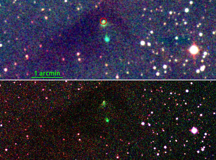
A&A proofs: manuscript no. main

1990, much of the wide-area effort depended on photographic              cluding a minority that did not meet all the desired survey qual-
emulsions on glass as detectors (e.g. the Palomar, ESO and UK-           ity criteria. The majority of the images included benefit from the
Schmidt sky surveys, described by Lund & Dixon 1973; West                uniform photometric zero points computed by Monguió et al.
1974; Morgan et al. 1992, respectively). The last thirty years           (2020) in building the IGAPS point-source catalogue.
has seen a switch to digital detectors that has brought with it              The structure of the paper is as follows. In section 2, we
the benefits of linearity and increased dynamic range, paving the        summarise the relevant features of IGAPS data and our methods
way for increasingly precise photometric calibration. Thanks to          and summarise the contents of the image database held within
this change and the advance of data science, the community now           http://www.igapsimages.org/. This is followed up by an outline
has access to a number of wide-area broad band surveys offer-            of the search tool available for querying the database (section 3).
ing images at ∼ arcsecond angular resolution and point-source            Attention then switches to our main focus: the properties and
catalogues (e.g. SDSS, Pan-STARRS, DECaPS, Skymapper: see                application of the narrowband Hα + [NII] imagery. Section 4
Alam et al. 2015; Chambers et al. 2016; Schlafly et al. 2018;            sets the ball rolling with an overview of the sensitivity and the
Wolf et al. 2018).                                                       nature of the background captured in the narrowband filter. We
    Wide-area narrow band Hα imaging, our main focus here,               then go on, in section 5 to highlight two contrasting examples
has generally been pursued separately from broad band work               of its exploitation for the science of diffuse nebulae (planetary
(most notably VTSS, SHASSA and WHAM, see Dennison et al.                 nebulae and Herbig-Haro objects). A discussion of techniques
1998; Gaustad et al. 2001; Haffner et al. 2003) . Finkbeiner             for mosaicking the Hα data then follows (section 6). Looking to
(2003) merged these surveys into a single map covering much              the near future of massively-multiplexed optical spectrographs,
of the sky, albeit at an angular resolution limited to 6 arcmin.         we present a method for automated searching of the IGAPS im-
Inevitably, most Hα nebulosity is concentrated in the Galactic           ages database for high Hα surface brightness non-stellar diffuse-
plane, along with most of the Galaxy’s gas, dust and stars. Within       ISM spectroscopic targets (section 7). To round off, we show two
the plane, the angular resolution needs to be better than this to        contrasting examples of the output from the automated search in
begin to resolve individual clusters and HII regions that show           section 7.4.
structure on the sub-arcminute scale. The UK Schmidt Hα Sur-
vey (SHS Parker et al. 2005), based on photographic film, has
met this challenge in the southern Galactic plane with imaging           2. Description of the image database
data of a resolution approaching 1 arcsec. Before the imaging
presented here began to be collected, the same could not be said         A series of papers (Drew et al. 2005; González-Solares et al.
for the plane in the northern hemisphere.                                2008; Groot et al. 2009; Barentsen et al. 2014; Monguió et al.
    The focus of this paper is on full coverage of the plane of the      2020) has already described the survey data acquisition and
northern Milky Way, via digital narrowband Hα imaging at ∼1              pipelining. So here it is only necessary to repeat pertinent de-
arcsec angular resolution obtained from 2003 up to 2018 using            tails.
the Wide Field Camera (WFC) on the Isaac Newton Telescope                     The camera used, the INT’s Wide Field Camera (WFC), is
(INT) in La Palma. We showcase the properties of the Hα images           a 4-CCD mosaic arranged in an L shape with a pixel size of
and point out different modes of exploitation, past, present and         0.33 arcsec/pixel. Each CCD images a sky region of roughly
future. Along side this, we also present the IGAPS 5-filter im-          11 × 22 sq.arcmin, giving a total combined field per exposure
age database, where IGAPS is the acronym for "The INT Galac-             of approximately 0.22 sq.deg. The five filters used – URGO , g, r,
tic Plane Surveys". IGAPS is the cross-calibrated merger of the          i, and a narrow-band Hα – have central wavelengths of 364.0,
two Galactic Plane surveys, IPHAS (The INT Photometric Hα                484.6, 624.0, 774.3, and 656.8 nm respectively. Despite the fil-
survey of the northern Galactic Plane, Drew et al. 2005), and            ter’s different naming, the URGO transmission curve quite closely
UVEX (The UV-Excess survey of the northern Galactic Plane,               resembles that of Sloan u (Doi et al. 2010). We shall refer to
Groot et al. 2009)1 . Together these surveys have offered a new          the narrow band filter as the Hα filter throughout this work, but
mix of narrow-band Hα alongside four broad bands spanning the            we note for completeness that the 95 Å bandpass also captures
optical. The IPHAS filters were r/i/Hα, while the UVEX survey            the [NII] 654.8, 658.4 nm forbidden lines typical of HII-region
incorporated a repeat in r and g/URGO observations. The total            emission. The numbers of CCD images per filter in the reposi-
IGAPS footprint is a 1850 sq.deg. strip along the Galactic Plane         tory are listed along with other performance parameters in Ta-
defined on the sky in Galactic coordinates by:- −5◦ < b < +5◦            ble 1. UVEX and IPHAS r band observations are distinguished
and 30◦ < ` < 215◦ .                                                     by labelling them rU and rI respectively.
    Monguió et al. (2020) have recently presented the merged                  IPHAS and UVEX shared the same footprint and set of
and calibrated IGAPS point-source catalogue of aperture pho-             pointings, such that the northern Galactic plane was covered via
tometry derived from the IPHAS and UVEX surveys. The focus               7635 WFC pointings, tessellating the survey area with, typically,
of this study was on the extraction of stellar photometric data. It      a small overlap. In addition, each field was observed again, and
did not take on characterisation of the extended ionised emission        usually around 5 minutes later, at an offset of +5 arcmin in RA
traced by the Hα images. This is the partner paper in which this         and +5 arcmin in Dec in order to fill in the gaps between the
missing piece is put in place.                                           CCDs and also to minimize the effects of bad pixels and cos-
    We will outline the world-accessible database of IGAPS im-           mic rays. As a result, almost all locations in the northern plane
ages we have set up to hold the Hα (and broad-band) data. It is          have been imaged twice in either survey. The presence of the r
reached via a website that also provides access to the Monguió           band in both surveys means that there will usually be at least 4
et al. (2020) point source catalogues. The imagery we have               CCD images, uniquely in this band, covering any given position
archived incorporates all IPHAS and UVEX observations in-                within the footprint. The only exception to mention is that there
                                                                         is a triangular patch of sky towards ` ∼ 215◦ where there are no
1
   In concept, these two surveys are the older siblings to VPHAS+,       UVEX URGO , g, rU images.
the survey covering the southern Galactic Plane and Bulge (Drew et al.        A distinction between the two surveys is that the blue UVEX
2014).                                                                   data were obtained during dark time, while IPHAS observations
Article number, page 2 of 21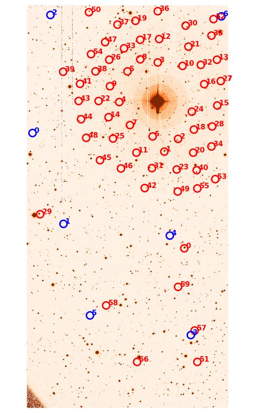
R. Greimel et al.: Hα northern Galactic plane imaging

  Filter    ING/WFC name            N       exposure                       PSF FWHM        sky count        ZP      5σ depth      moon phase
                                            (sec)                            (arcsec)                     (mag.)     (mag.)
  i         WFCSloanI             83652     10 (83%), and 20 (17%)             1.06                92      26.42      20.28           0.68
  Hα        WFCH6568              83652     120                                1.20                57      26.57      20.40             "
  rI        WFCSloanR             83652     30 (85%), and 10 (15%)             1.16               164      28.19      21.37             "
  rU        "                     67896     30                                 1.18               126      28.20      21.67           0.21
  g         WFCSloanG             67895     30                                 1.26                61      28.71      22.38             "
  URGO      WFCRGOU               67892     120                                1.48                43      27.85      21.47             "
Table 1. Properties of the repository contents by filter for the better-quality image sets graded A to C. The number N specifies the number of CCD
images available in the A to C grade range for each filter (D-grade images with identified problems, are not included in the count). Median values
are listed for the full width half maximum of the point spread function (PSF FWHM), the sky background count, zeropoint (ZP), 5σ detection
limit in the Vega system, and moon phase. The PSF FWHM and the background count are pipeline measures, while the zeropoint and limiting
magnitude are based on the uniform calibration (Monguió et al. 2020). Moon phase is given as a fraction, such that 0 corresponds to new moon
and 1 to full moon. The rI exposure time started out at 10 sec, but was raised to 30 sec from 2004 on, while the i exposure time was increased to
20 sec starting in October 2010.

were generally made with the moon above the horizon. This dif-             In the AB magnitude system this is equivalent to a magnitude of
ference means that background sky counts are typically higher in           0.328.
the red IPHAS images than they are in UVEX images. A prac-                     Expressed in point-source magnitudes the bright limit of the
tical consequence of this is that UVEX rU data go deeper than              images is in the region of 11–12 in i and Hα, rising to 12–13 in
IPHAS rI by 0.3 magnitudes, on average (see Table 1). Another              the more sensitive r and g bands. There were specific observation
impact is that the background levels in the brighter-time observa-         periods in which WFC electronic issues meant that saturation
tions in the Hα filter can exhibit marked variation, depending on          was reached at appreciably lower count levels than the norm.
how far away and full the moon is and on cloud cover (see sec-             For example, there was a particular problem affecting CCD 2 in
tion 4). These variations, especially when mixed with Hα neb-              November 2006 that would push the bright limit fainter by up to
ulosity, represent a challenge when mosaicking IPHAS data to               a magnitude. Users of the data can track such problems in the
build large-area images. How this challenge can and has been               images via the count level recorded against the header keyword,
met is the subject of section 6.                                           SATURATION.
    A part of the pipelining procedure for all survey data was to              As part of creating the point source catalogue images were
apply a flux calibration based on nightly standard-star observa-           graded from best to worst as A++, A+, and A to D. For a defi-
tions. The zero points, in the Vega system, obtained on this basis         nition of the grades see appendix A in Monguió et al. (2020). A
remain associated with all images in the repository and are stored         last point to make about the images is to note that, while there
in every image header as the keyword MAGZPT. The meaning                   is minimal vignetting of CCDs 1, 2 and 4, there is persistent vi-
of MAGZPT is that it is the magnitude in the Vega system of                gnetting of the corner of CCD 3 furthest from the optical axis of
an object giving 1 count per second (it does not fold in the ex-           the WFC (which passes through CCD 4). In Appendix A.2 a typ-
posure time). For details of how it is derived see equation 4 in           ical confidence map is shown to illustrate this. In Appendix A.3,
González-Solares et al. (2008). Experience showed that broadly             we briefly outline common artefacts in the image data.
consistent and reliable results were obtained for the URGO and
Hα filters if their zero points were fixed at a constant offset rel-
ative to (respectively) their partner g and rI frames. For URGO            3. Accessing the images
this is the only calibration presently available. For g, rU , rI , i and   All the reduced images from both surveys can be accessed
Hα, a uniform recalibration of the photometry was undertaken in            via the website, http://www.igapsimages.org/, hosted by Univer-
preparing the point source catalogue (Monguió et al. 2020). The            sity College London. Altogether the repository contains 527736
result of this is that around 2/3 of the images in the repository          CCD frames, of which 314923 (or 60%) carry the best-quality A
now carry a revised zero point (PHOTZP header keyword) that                grades and 73097 (14%) are minimum-quality D graded. These
rests on a comparison with PanSTARRS g, r and i photometry.                grade assignments were made at the level of the basic unit of ob-
This zero point has incorporated the image exposure time, which            servation in the two constituent surveys – the consecutive trio of
means it is the magnitude of a source giving 1 count integrated            exposures obtained at each sky position. The details of the grad-
over the exposure. Hence, the Vega magnitude of any imaged                 ing system at work in evaluating data for the IGAPS catalogue
source can be computed from:                                               can be found in Appendix A of the catalogue paper (Monguió
                                                                           et al. 2020). A consequence of this approach, also applied to the
m = −2.5 log(enclosed counts) + PHOT ZP                             (1)    earlier IPHAS DR2 release (Barentsen et al. 2014), is that the
where, for a point source, the enclosed counts would be the total          grade assignment, referred to individual CCD frames or even fil-
counts within a user-specified aperture, after subtraction of an           ters, can be pessimistic, as it takes just one substandard exposure
estimate for the enclosed underlying background.                           in a set of three to pull down the grade for all of them. In view of
     The Hα filter magnitude scale is not one conventionally de-           this, and the occasional scientific value of maximising the num-
fined within the Vega system. This means we need to define the             ber of images to examine, the decision was taken to retain all D
flux corresponding to the zero of the magnitude scale appropriate          graded data in the repository, alongside the A to C graded expo-
to it. We determine that the zero-magnitude flux entering the top          sures.
of the Earth’s atmosphere within the WFC Hα filter transmission                The images access page within the website offers a search
profile is                                                                 tool that enables users to search for and download images that
                                                                           either overlap a single specified position or occupy a square box
F[m(Hα) = 0] = 1.57 × 10⁻⁷ ergs cm−2 s−1 .                          (2)    of size up to 1 × 1 sq.deg. on the sky. The user can choose the
                                                                                                                     Article number, page 3 of 21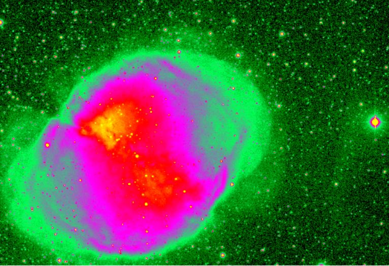
A&A proofs: manuscript no. main

      Quantity                                   Percentiles                    Figure 2 shows how the recorded sky background count lev-
                                             5       50      95            els convert into narrow-band Hα surface brightness, via the set
                                                                           of zeropoints, PHOTZP. The plot includes only data that have
      Counts                                27       52      210           passed through the uniform photometric calibration. Most of the
                                                                           data conform reasonably well to a linear trend such that 1 count
      Vega magnitude                                                       per pixel corresponds to 3.32 × 10⁻¹⁷ ergs cm−2 s−1 arcsec−2
      (mag arcsec−2 )                      20.6     19.9     18.3          (or 5.9 Rayleighs)2 . The absolute minimum sky brightness mea-
                                                                           sured in any calibrated frame is 6.6×10⁻¹⁶ ergs cm−2 s−1 arcsec−2
      Surface brightness                                                   (∼ 120 Rayleighs), but it is commonly more than twice this. Sky
      (10−15 erg cm−2 s−1 arcsec−2 )       0.91     1.7       7.4          transparency necessarily influences the behaviour. At times of
                                                                           reduced transparency the sensitivity suffers, driving data points
Table 2. Percentiles of the distribution of narrowband Hα+[NII]            from affected nights onto steeper linear trends in Figure 2.
pipeline-computed background levels in uniformly-calibrated images.             Figure 3 is a plot of the pipeline measurement of sky noise
The sample used here numbers 63956 CCD frames (or 15989 WFC                versus the estimate of sky background, both in counts per pixel.
exposures). Not included are the 36808 CCD frames (9202 WFC expo-          For around a half of the uniformly calibrated frames, the noise
sures) for which only the pipeline photometric calibration is available.   is limited to under 6 counts per pixel (or ∼ 2 × 10⁻¹⁶ ergs cm−2
                                                                           s−1 arcsec−2 ), and it is extremely rare that the sky noise is more
                                                                           than ∼12 counts per pixel. A simple expectation for the form of
filters of interest and decide whether to omit grade D data. In            the relation between sky noise and level is
response to a query, the tool returns a table listing the images                                    √
                                                                           Nbg = (NRN + Cbg )/ n pe
                                                                                           p
                                                                                                                                           (3)
meeting requirement, along with key metadata (grade, seeing,
depth, whether calibrated) that can inform the user’s final choice         where Nbg and Cbg are respectively the sky noise and sky level,
of images for download. For convenience, there is a column of              NRN is the CCD read noise, also in counts per pixel, and n pe rep-
tick boxes in the table, that allows the user to deselect some of          resents the effective number of pixels over which the sky statis-
the listed images before initiating the download of a gzipped or           tics are measured. Basically, we expect the noise to be the sum of
tarred collection of Rice-compressed (.fz) images.                         a constant and a Poisson component. In practice, the sky level is
     It is generally the case that a contemporaneous rI image ac-          determined numerically by the pipeline using two-dimensional
companied an Hα and i image of the same pointing. Similarly                non-linear background tracking across the full CCD at a super-
the UVEX rU , g and URGO images were observed as consecu-                  pixel level. After the background fit has been subtracted from
tive triplets. Given that stars are sometimes subject to variability,      an image, the sky noise is calculated iteratively from the clipped
users of the repository may need to bear this in mind when de-             median absolute deviation (MAD) of the residuals.
ciding how to select images for scientific exploitation.                        As the readnoise for the WFC is known to be NRN = 2.37
     The website also provides a link to a large table of metadata         counts, we only need to fit one parameter of this function. Be-
that previews the header information provided with the full set            fore the fitting, outliers above the dashed line in Figure 3 were
of image profiles.                                                         removed. The fit was performed using an iterative 3-σ clipped
                                                                           Levenberg-Marquardt algorithm using the median and MAD in
                                                                           place of mean and σ. The result of the fit is
4. Properties of the Hα images: backgrounds and                                                     √
                                                                           Nbg = (2.37 + Cbg )/ 2.88 = 1.4 + 0.589 Cbg
                                                                                           p                             p
   sensitivity                                                                                                                             (4)
                                                                           Allowing an additional     fit parameter, namely a multiplicative
At the outset, the IPHAS survey was allocated time on the ex-                             p
pectation the programme could cope with a moonlit sky. After               factor for the Cbg term, does not lead to a statistically signif-
the first few seasons and some experience had accumulated, the             icant improvement in the fit, and the factor is found to be very
brightest nights were increasingly avoided. Indeed, in the late            close to 1. Hence we are confident that equation 3 accurately
stages when the acquisition of the blue UVEX filters took prior-           describes the distribution.
ity, dark and grey nights became the norm. The net result is that              In presenting the Schmidt Hα Survey, Parker et al. (2005),
the median background level among all the uniformly-calibrated             compared its sensitivity with IPHAS and other available Hα
Hα images is closer to grey, than bright. Table 2 provides some            wide-area surveys. In their Table 1 it was estimated that the depth
numerical detail illustrating the strongly skewed distribution fi-         reached by the narrowband (IPHAS) data presented here is ∼3
nally achieved. For comparison with the magnitudes in the table,           Rayleighs. This is a surface brightness of 1.7 × 10⁻¹⁷ ergs cm−2
we mention that the ING exposure time calculator uses 20.6,                s−1 arcsec−2 or, as required by the mean calibration illustrated
19.7 and 18.3 mag arcsec−2 to represent dark, grey and bright              in Figure 2, the equivalent of around a half count per pixel in a
sky in the R photometric band – values closely resembling the              120 sec exposure at the typical 1 to 1.5 arcsec seeing. The on-
tabulated 5th, 50th and 95th percentiles.                                  sky solid angle that the Parker et al. (2005) estimate refers to was
     Around a third of the images were not passed through uni-             not made explicit – clearly it cannot be 1 arcsec2 . If we assume
form calibration: of these (generally inferior) data, just under a         Cbg = 0.5 counts pixel−1 at 3 σ, Nbg = 0.5/3, we can use equa-
third have background levels in Hα exceeding the 210 counts                tion 3 to calculate the pixel area needed to achieve a sensitivity
marking the 95th percentile of the uniformly-calibrated set of             of 3 Rayleighs. We obtain 18.5 × 18.5 pixels or 6.1 × 6.1 arcsec.
images. Most of them were obtained early on in the survey, and                 Used at full seeing-limited resolution, the Hα data provide
most have been repeated, resulting in calibrated alternatives. Just        safe detection of raised surface brightness due to diffuse-ISM
339 calibrated Hα exposures (1356 CCD frames, or 2 percent                 emission at the level of a few times 10−16 ergs cm−2 s−1 arcsec−2 ,
of the total) are left without alternatives in the database, where         or 50–100 Rayleighs. That this is so will be demonstrated by
the background count exceeds the 95th percentile of 210 counts.            different means in section 7.
Where these sit in the survey footprint is shown in Figure 1.              2
                                                                               At Hα, 1 Rayleigh is equivalent to 5.67×10⁻¹⁸ ergs cm−2 s−1 arcsec−2

Article number, page 4 of 21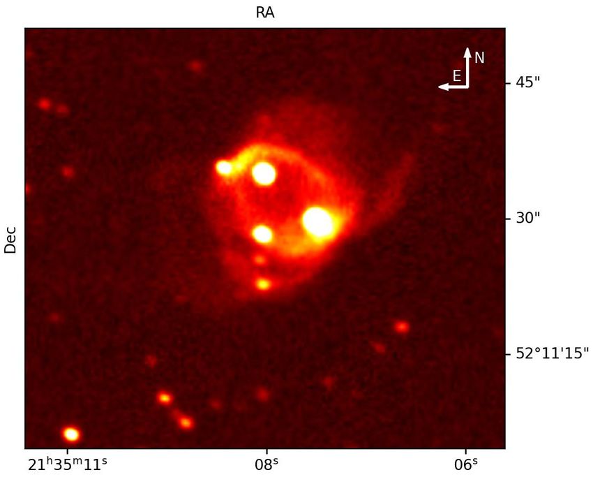
R. Greimel et al.: Hα northern Galactic plane imaging

Fig. 1. Map of the uniformly-calibrated IGAPS field centres (grey). A darker grey colour is seen where the database contains more than one
uniformly-calibrated exposure. The orange overplotted points mark the 339 exposure sets (1356 CCD frames), without alternatives in the database,
where the Hα sky background exceeds 210 counts (> 95th percentile).

Fig. 2. Density plot of background surface brightness in the Hα band        Fig. 3. Density plot of the pipeline-measured sky noise in the Hα filter
as a function of measured mean sky level in counts. The colour scale        as a function of sky level. Both are in units of counts per pixel. The
is logarithmic, with blue representing the highest density of points. The   coloured data shown, and plotted on a logarithmic density scale, are
images used to build this diagram are the IGAPS uniformly-calibrated        drawn from the IGAPS uniformly-calibrated set. The solid black line
set, which enables validated conversion of the sky counts to surface        is the fit discussed in the text, given as equation 4, that shows the sky
brightness via each image’s zeropoint. The black dashed line has a gra-     noise increases mainly as the square root of the sky level. The lighter
dient of 3.32 × 10⁻¹⁷ ergs cm−2 s−1 arcsec−2 per count.                     grey data (underneath) are from images with zeropoints that were not
                                                                            passed through uniform photometric calibration.

5. Exploitation of the Hα images
                                                                            via plasma diagnostics (density, temperature, velocity and so on)
The search for and characterization of extended nebulae was an              and the chemical composition allows the measurement of their
original goal of the IPHAS component of the merged IGAPS                    impact on the chemical enrichment of any given galaxy. How-
survey. Initially this mostly concentrated on planetary nebulae             ever most of the known PNe are bright and/or nearby as the faint
(PNe). Discoveries of examples of those alternative products of             ones have been ignored or are out of reach due to observational
end-state stellar evolution – supernova remnants – have also been           constraints. An aim of IPHAS was to perform a near complete
found and recorded (Sabin et al. 2013).                                     census of the PNe in the northern Galactic Plane, where a higher
    Below we present brief discussions of how nebulae can be                concentration of ionised sources co-exists with high extinction.
found and studied, taking the contrasting examples of new PNe               Progress towards this goal has been described by Sabin (2008)
and – from the more obscured first phase of the stellar life cycle          and Sabin et al. (2014).
– a Herbig Haro object.
                                                                            5.1.1. Detection Methods
5.1. Planetary nebulae
                                                                            Depending on the size of the sources two methods were adopted.
Planetary nebulae (PNe) are the end-products of low and in-                 On the one hand, compact or point-source PNe have been se-
termediate mass stars (∼1–8M ) where a hot central star fully               lected based on Hα excess as measured and recorded in pho-
ionises its surrounding shell leading to a glowing nebula. These            tometric catalogues, and cross-checked against IR photometry
objects are ideal tools to study the later stages of stellar evolu-         (e.g. 2MASS, see Viironen et al. 2009). On the other hand, for
tion as most stars in our Galaxy will go through this phase. We             the case of extended PNe, a mosaicking process was developed
can access information related to their physical characteristics            using 2◦ × 2◦ Hα − r mosaics with 5×5 pixels and 15×15 pix-
                                                                                                                       Article number, page 5 of 21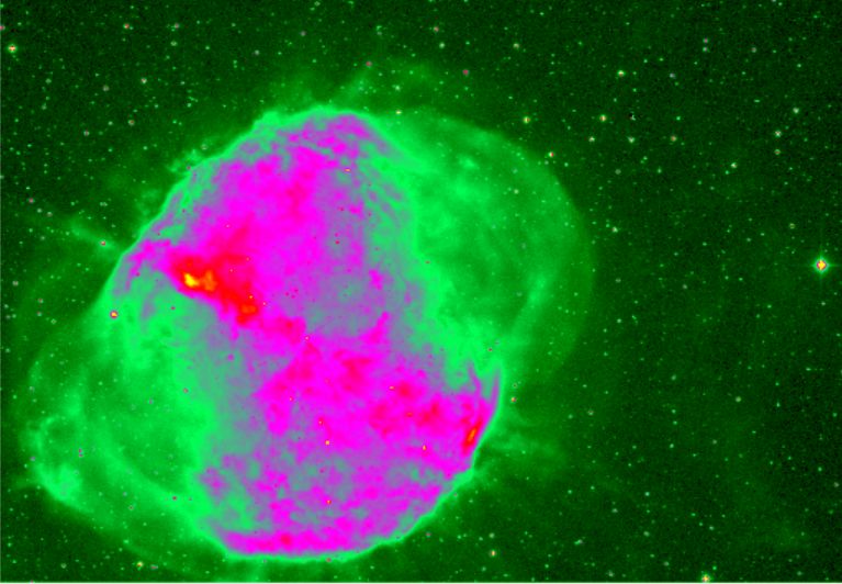
A&A proofs: manuscript no. main

els binning factors (corresponding to ∼1.7 and ∼5 arcsec effec-
tive pixel sizes respectively, see Sabin 2008). The coarser bin-
ning was mainly used to detect large and low-surface brightness
nebulae, while the lower binning was aimed at detecting smaller
nebulae hidden in crowded stellar fields. In the latter case we
also used the technique adopted in the southern MASH survey
(Parker et al. 2006; Miszalski et al. 2008) where RGB composite
imagery (Hα, r’ and i’ filters) is used to distinguish stars from
diffuse ionised nebulae.3 Always, new objects were confirmed
by independent eyeballing of the data by several team members.
    This task was found to be ideal for undergraduate projects
and two example discoveries are shown below.

5.1.2. New Discoveries
Hundreds of new PN candidates were found as a result of
the visual search with the mosaics and a first large spectro-
scopic follow-up involving no less than nine world wide tele-
scopes/instruments ranging from 1.5m (ALBIREO spectrograph
at the Observatory of Sierra Nevada, Spain) to 10.4 m (GTC-
OSIRIS spectrograph at the Observatorio del Roque de los
Muchachos, Spain) was conducted (Sabin et al. 2014). We iden-
tified 159 objects as True (113), Likely (26) and Possible (20)
PNe and unveiled a large range of shapes (mostly elliptical, bipo-
lar and round PNe) and sizes (up to ∼8 arcminutes).
     Among all the newly detected PNe, some caught our at-                Fig. 4. IPHASXJ015624.9+652830: this is a cutout from one of the 2
tention first due to their outstanding morphology and then due            by 2 degree binned Hα-r mosaics used for searching for new PN.
to their interesting characteristics revealed by subsequent deep
analyses. Notable examples include: the knotty bipolar IPHASX
J194359.5+170901, now known as the Necklace Nebula (Cor-
radi et al. 2011); the quadrupolar IPHASX J012507.9+635652
(alternately named Príncipes de Asturias by Mampaso et al.
2006); IPHASX J052531.19+281945.1 at large galactocentric
distance (Viironen et al. 2011); and finally, the PN discovered
around the nova V458 Vul (Wesson et al. 2008). IPHAS, and
now IGAPS, also allows us to target the particular group of PNe
interacting with the interstellar medium (ISM). Those objects
which are slowly diluting in the ISM are particularly difficult to
detect most of all in their late phase. In this case IPHAS imaging
data can reveal such faint material (Sabin et al. 2010).
     We show in Figures 4 and 5, two of the many new PNe that
have been found and have not yet appeared in the refereed liter-
ature. Most of the new finds are published in Sabin et al. (2014).
The first object IPHASXJ015624.9+652830 (PNG 129.6+03.4),
shown in Figure 4, came from parallel searches of the 15 × 15
pixel binned Hα − r (5 arcsec per pixel) mosaics, carried out by
team members and undergraduate students supervised by them
in 2007. This object can be seen in the Hα images but is easily           Fig. 5. PNG 95.3+0.2: this is a cutout from one of two CCD frames
missed, yet it stands out very clearly in the binned difference im-       downloaded from the IGAPS image archive. The alternative available
ages as the only object in an otherwise blank frame. This demon-          image of the PN (not shown) happens to sit adjacent to a ’bad line’ in
strates the usefulness of this method for the discovery of new            the CCD. It is precisely to mitigate against this kind of problem that
objects, especially those that, like this one, are only detectable in     the survey strategy was to collect data from paired offset pointings. The
optical wavebands.                                                        object IPHAS J213508.15+521128.0, discussed in the text, is the lower
     The second nebula, PNG 95.3+0.2, shown in Figure 5, was              left of the three bright stars in the central region of the nebula.
discovered using the same search method by Fernández-Martín
(2007). Subsequent high resolution (0.6 arcsec seeing) imaging
with the NOT telescope on the night of 4th September 2007,                especially well in the [NII]-only image. Since the IPHAS Hα fil-
through Hα, [OIII] 5007Å, and [NII] 6583Å filters further clari-          ter bandwidth also incorporates this line, Figure 5 is a compos-
fied an intricate morphology with a bright, roughly elliptical cen-       ite image, showing both the [NII]-dominated outer filamentary
tral shell, and a pair of fainter twisted protrusions that show up        structure and the Hα dominated inner ellipse.
                                                                               PNG 95.3+0.2 is now listed in the HASH Catalogue of
3
   With advances in the use of machine learning, the classifications of   Parker et al. (2016). It is associated with an infrared (WISE,
objects in the HASH database can now be automated (Awang Iskandar         and 90µm AKARI), and 1420 MHz radio source (Taylor et al.
et al. 2020)                                                              2017). According to Anders et al. (2019), the G ' 17.1 mag
Article number, page 6 of 21
R. Greimel et al.: Hα northern Galactic plane imaging
star near the geometrical centre, IPHAS J213508.15+521128.0,
or Gaia EDR3 2171830374492778880, is a distant, reddened,
and apparently relatively cold star (D = 5.5± 0.9 kpc, AV =
3.9 ± 0.2 mag, Teff = 4800 ± 260 K). However, our evalua-
tion of the IGAPS broad-band photometry (Monguió et al. 2020)
is that the available magnitudes are also consistent with this
object being a much hotter, even more extinguished star. The
other two, brighter stars embedded in the nebula are located in
the foreground at much more secure parallax-based distances of
0.9 and 1.6 kpc: in the Anders et al. (2019) database, they too
are assigned low Teff values, incompatible with those of a hot
PN central star. Vioque et al. (2020) combine IPHAS, 2MASS
and WISE data in a search for new Herbig Ae/Be stars and list
IPHAS J213508.15+521128.0 as a non-Herbig AeBe, non-pre
Main Sequence, and non-classical Be star – nor do they confirm
an association with a PN (their FPN flag is empty). The WISE
source, detected in the four bands and centered at 1.1 arcsec from Fig. 6. Top: RGB image (epoch 2007) of the dark cloud Dobashi 3782,
IPHAS J213508.15+521128.0, shows red IR colours like known based on I, Hα, and [S II] frames taken with the Tautenburg Schmidt
PNe, while the spectral energy distribution of the star, built from telescope. It hosts the YSO IRAS 01166+6635, marked by the circle,
Pan-STARRS, 2MASS, ALLWISE, and AKARI data, is typical which drives a jet that excites a compact HHO south of it (centre). It ap-
of a reddened star up to the WISE W3 (12µm) band. Beyond that, pears greenish-blue in this RGB representation because of its strong Hα
emission. Bottom: IGAPS RGB image (epoch 2013), based on i, Hα,
a strong IR excess appears up to 90µm, and points to a physical and rI frames. The YSO, as well as the HHO, appears green because it
association of IPHAS J213508.15+521128.0 with the nebula. If is not clearly detected in either rI or i. The HHO is just resolved at no
that is the case, the apparent nebular size of around 30 arcsec more than 2 arcsec across.
would imply a rather large, evolved nebula, 0.8 pc in diameter,
and also suggest the existence of a hidden hot star (a binary?) in
the surroundings. PNG 95.3+0.2 is an appealing example of an tions (PMs) and radial velocities (RVs) allow a kinematic dating
IPHAS extended object with plenty of online, publicly available of the ejection event. Moreover, such data provide information
information, that nevertheless deserves further dedicated obser- on the inclination i of the circumstellar accretion disk. Constrain-
vations including careful quantitative spectroscopy to pin down ing the latter is crucial for the analysis of YSO spectral energy
the central star. distributions using radiative transfer modelling.
Basic confirmation spectra exist for both the above neb- The potential of IGAPS for such studies is illustrated by
ulae. The objects have also been independently discovered the example of a hitherto unknown HHO, driven by IRAS
more recently by amateur astronomers. The first object, 01166+6635. This low-mass YSO (Connelley et al. 2008) is
IPHASXJ015624.9+652830, has also come to be known as Fer- emerging from the small dark cloud, Dobashi 3782, situated
rero 6, Fe6, PN G129.6+03.4, while the second, PNG 95.3+0.2, at a kinematic distance of 240 pc (Wouterloot & Brand 1989).
is also known as StDr Objet 1. Full details on both can be found Narrow-band imaging performed in 2007 with the Tautenburg
in the HASH database (Parker et al. 2016). Schmidt telescope revealed a compact HHO south of the YSO
within ∼1 arcsec of the position RA 01:20:02.9, DEC +66:51:00
(J2000) (Fig. 6). The estimated extinction out to the distance of
5.1.3. Previously known PN this cloud is about AV ∼ 2.5, averaged across a few arcminutes
(Sale et al. 2014). The extinction towards the optically-faint YSO
The survey is also useful for the re-analysis of already known is without doubt much more. At the position of this YSO there
PNe. IPHAS images can unveil new faint structures associated are eight entries in the IGAPS catalogue (Monguió et al. 2020)
with known PNe that have hitherto evaded detection. A clear within a radius of 5 arcsec. Six of the eight are Hα only sources.
example of this is the detection of the extended tail of the known Blinking with the POSS1 red image showed evidence for
Sh 2-188 by Wareing et al. (2006) which enabled the reeval- proper motion within ∼50 years. Thus, in order to establish
uation of its full extent. A different application has recently its kinematics, Hα and R-band frames have been secured for
been presented by Dharmawardena et al. (2021): with a view to as many epochs as possible. Four Hα frames with grade A
appraising different methods of determining PN distances, they quality (r367494 and r367497 obtained 2003, r1018994 and
have collected IPHAS Hα+[N ii] aperture photometry fluxes for r1018997 obtained 2013) were retrieved from the IGAPS im-
151 previously known nebulae as well as for 46 confirmed or age server. These are supplemented by archival Tautenburg Hα
possible PNe that had been discovered by the IPHAS survey. images (2007, 2012) and two frames taken in 2020 with the new
TAUKAM instrument (Stecklum et al. 2016). The POSS 1 and
2 R-band images (1954, 1991) were added as well, using both
5.2. HH-objects plate digitisations from STSci and SuperCosmos. Before deriv-
ing the HHO positions by fitting its image profile, all frames
During their growth, young stellar objects (YSOs) eject a frac- were tied to the Gaia EDR3 astrometric reference system (Gaia
tion of the in-falling matter at high speed via bipolar jets and Collaboration 2020).
outflows. Their shock fronts, delineated by line emission, par- The coordinate offsets of the HHO relative to the driving
ticularly in Hα, [SII], and [OI], are called Herbig-Haro objects source for the various epochs are shown (Fig. 7), along with
(HHOs, Herbig 1950; Haro 1952). HHOs not only trace the pres- their respective linear fits. For the distance given above, the DEC
ence of young stars, but can also serve as a record of their accre- slope (red) corresponds to a velocity of −91.0 ± 3.5 km s−1 . As-
tion history. The kinematics of HHOs, derived from proper mo- suming constant speed, this implies a kinematic age of ∼430 yr.
Article number, page 7 of 21A&A proofs: manuscript no. main
chips. This wave-like structure contributes ∼2% of the total
counts in some images (Irwin & Lewis 2001). It is almost en-
tirely removed in the CASU pipeline (who use a library of i-band
fringe frames from other INT WFC observing runs), although
some will remain at the ∼0.2% level due to night-to-night vari-
ations. When i-band data is mosaicked, overlapping fringing is
occasionally exaggerated and can remain visible in some mo-
saics.
As noted in Section 4, IPHAS observations were at first car-
ried out at any level of moon brightness throughout the Galactic
plane season. Observations during bright time were soon found
to exhibit varying levels of background counts in the form of a
small but noticeable gradient across each CCD (leading in later
Fig. 7. HHO position displacement with regard to the ALLWISE posi- seasons to tighter moon phase and distance requirements). Ulti-
tion (Cutri & et al. 2014) over time (red - DEC, blue - RA). The respec- mately, ∼8% of all IPHAS images were taken under such condi-
tive regression lines are shown as well. tions.
Moonlight affects IPHAS images through both scattered
light across the night sky and a component that reflects off the
It is likely a major accretion event happened around that time
inside of the telescope dome and across the CCD array. The re-
which induced jet strengthening. Accounting for the position an-
sulting illumination is therefore not necessarily uniform across
gle of the HHO movement of 190◦ (measured from N through E),
all four CCDs, and requires a CCD-by-CCD solution. Its char-
a total PM speed of 92.4 ± 3.5 km s−1 can be derived. With the
acter is also influenced by the phase of the moon, its altitude
help of an RV estimate of −74.8 ± 4.6 km s−1 , obtained by low-
above the horizon, angular separation from the pointing of the
resolution spectroscopy of the HHO using the Nasmyth spectro-
telescope, and the extent (and position) of cloud cover across the
graph at the Tautenburg telescope, the inclination of the velocity
sky. These relatively small gradients can be exacerbated by mo-
vector follows as 51◦ ± 2◦ . This intermediate inclination is con-
saicking CCD images over large areas of the sky (many degrees),
sistent with the cometary appearance of the YSO in the optical.
becoming a significant issue in the production of large mosaics.
This example shows that the IGAPS Hα line emission im-
The recommended solution to removing the moonlight and
ages provide an excellent means for the detection of HHOs.
achieving a flat and dark background is to model and fit the
In this instance, neither the driving YSO nor the HHO are de-
background gradient for each CCD. Since the r and Hα band
tected even in i-band, and yet the detection of the HHO in Hα
images contain nebulosity that could affect the fit, we recom-
is clear, at around 30 counts above background (depending on
mend fitting the background gradient to r − Hα images (after
the seeing). Moreover, the 1-arcsec resolution of IGAPS images
scaling the images to correct for their different exposure times),
allows for good position measurements of these small (but ex-
since both filters contain the Hα and forbidden [Nii] lines that
tended) nebulous objects. Together with the availability of re-
typically dominate diffuse astronomical emission. Binning the
peated IGAPS observations, with several years of epoch differ-
image into 100 × 100 pixel bins and taking the median pixel
ence, precise proper motion measurements are possible, from
value in each bin provides a simple method to measure the back-
which information about the physics of the HH flows, as well
ground level in that bin. A two-dimensional gradient of the form
as their driving sources, can be obtained.
Z = Ax + By + C can then be fit to the data, where A, B and C
are free parameters, using, for example a Markov Chain Monte
Carlo simulation and the Python code emcee (Foreman-Mackey
6. Image mosaics
et al. 2013). More complex models have been tested (including
The background of astronomical images would ideally be flat Fourier transform techniques), but none were found to provide a
and dark. In reality the background in images from ground-based significant improvement. In short, the two-dimensional gradient
telescopes varies due to the interplay of different sources (e.g., method will prove effective in the majority of cases.
airglow, moonlight) contributing varying levels of unwanted Some care should also be applied when very bright stars fall
light. on (or near) one of the CCDs, as saturation, atmospheric and
To begin to tackle this securely, when working with the stan- lens effects can heavily affect an image and the model fit to it.
dard image data reduction available in the database, we recom- Identifying and excluding a magnitude-dependent radius around
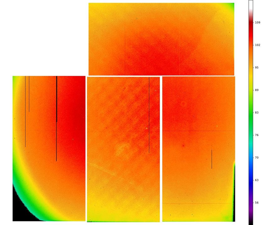
mend using the available confidence maps to reject pixels with such stars using the Tycho-2 catalogue of bright stars (Høg et al.
confidence levels less than 90-95% typically. But we note that 2000) proved effective for overcoming these problems.
the level can vary across the sky and between filters, usually re- As an example of the potential of IGAPS image mosaicking,
quiring a lower confidence level threshold for the g filter and we present a large, 4.2 × 3.6 degree Hα mosaic of the supernova
especially URGO . remnant Simeis 147, produced using the techniques described
The Montage software4 can be used to effectively mosaic above. Simeis 147 (hereafter S147) is otherwise known as SNR
images in a given filter, re-projecting images as needed to a G180.0-01.7, Shajn 147, or Sharpless 2-240. It is a large, faint,
single-projection algorithm and direction, adjusting the back- late-stage remnant located just below the Galactic Anticentre.
ground levels in overlapping pairs of images to produce a smooth It was discovered in 1952 and lies at a distance of 0.8–1.6 kpc
mosaic over a large area. (Gvaramadze 2006), on the near side of the Perseus spiral arm.
In addition to uniform background light sources, the i-band The SNR consists of numerous filaments embedded in large-
can sometimes be beset by fringing that originates from the air- scale diffuse emission. The east and west edges of S147 show
glow OH lines interfering via internal reflections in the CCD signs of blow-outs, the southern edge shows a sharp boundary,
with a less regular one in the north. The undistorted appearance
4
Available from http://montage.ipac.caltech.edu/ of the SNR may partly be due to it expanding into a region of
Article number, page 8 of 21R. Greimel et al.: Hα northern Galactic plane imaging
Fig. 8. Supernova remnant, S147. This is a full resolution background-corrected mosaic made from the Hα-filter data (no r subtraction). Approxi-
mate image dimensions are 4.2 × 3.6 sq.deg. North is up and east is to the left. The greyscale is negative such that the brightest emission is darkest.
Compared to the earlier mosaic appearing as Figure 19 in Drew et al. (2005), based on Hα − r data, with background fitting and removal, there
are fewer artefacts thanks in large part to the incorporation of better re-observations. Much of the faint structure left, such as the ragged diffuse
emission in and below the centre of the remnant,is real.
space already partly cleared by a previous supernova (Gvara- ESO at Paranal (de Jong et al. 2019). Both facilities will collect
madze 2006). Regardless, examples of large and pristine SNRs on the order of 1000 targets per pointing, and a major science
are rare and observations of them can be important for constrain- driver for both is Milky Way science in the Gaia era.
ing hydrodynamic simulations of their expansion and structure. Massive-multiplex spectroscopy requires informed target se-
Figure 8 shows the full mosaic constructed as outlined above. lection. The IPHAS Hα images, in particular, can characterise
The challenge of this object is its great size, allied with very the diffuse sky for studies of the ionised ISM. Here, we out-
intricate and sometimes very faint small scale detail. The number line a software method – named HaGrid – aimed at doing this
of individual CCD frames included is in the region of 250. The through the interrogation of Hα images. The positions gener-
full-resolution S147 mosaic (199 MB) itself is provided as a fits- ated by HaGrid will be used in constructing the SCIP (’Stellar,
formatted file attached to this paper as supplementary material. Circumstellar and Interstellar Physics’) northern Galactic plane
programme – a strand within the overall WEAVE 5-year sur-
vey. The software is also being deployed to find targets for the
7. Nebular target selection for massive-multiplex southern plane (based on VPHAS+ data), to enable similar ob-
spectroscopy servations via 4MOST. In the text below, the acronym WEAVE
appearing on its own will stand both for the instrument and for
The next decade will see an increase in large, multi-object digi-
the WEAVE/SCIP survey strand, according to context.
tal spectroscopic surveys on 4m class telescopes. In drawing up
target lists, these surveys will make use of the data that has been
acquired by wide-area digital photometric surveys, like IGAPS. 7.1. Building lists of science targets with HaGrid
Two examples due to start soon are the WEAVE survey on the
4-metre William Herschel Telescope (WHT) of the Roque de los A WEAVE pointing is defined by the coordinates of its centre
Muchachos Observatory in La Palma (Dalton et al. 2020) and and a field of view of radius of 1 degree, projecting a circle on the
the 4MOST survey on the 4-metre VISTA telescope operated by sky covering π sq.deg. Within such a field, the aim is to identify
Article number, page 9 of 21A&A proofs: manuscript no. main
several hundred positions that coincide with regions of (locally)
maximum Hα brightness.
In outline, the steps taken are as follows:
– Find all Hα CCD images from the IGAPS repository in the
area of interest.
– Mask out stars, CCD borders, bad pixels and vignetted areas
from the data.
– Divide the image into superpixels.
– Select the superpixels with the highest counts as candidate
source positions.
The application of the algorithm, confronted with real data,
is necessarily more complicated, particularly as it must deal as
far as possible with all the artefacts that mimic real nebulosity.
So we now itemize the steps involved in more detail:
– Collect the CCD images from the IGAPS repository in the
Fig. 9. Left: Ghost on image r372056, CCD#4 due to a bright star. No-
area of interest. For one WEAVE field of radius 1 degree, tice the stray-light image even picks up details of protruding cabling at
this will be a list of over 100 Hα CCD frames and their prime focus of the INT. Part of a much fainter ghost can be seen top
associated rI exposures. Since frames with poor data qual- right. Right: Example of a halo around a bright star fooling the HaGrid
ity often lead to false detections of Hα emission, we ex- selection from r541554 CCD#3. Source positions selected by HaGrid
cluded, where possible, grade C and D frames and favoured are shown as red numbered circles. They crowd into the faint extended
uniformly-calibrated over pipeline-calibrated data. halo that is a little offset from the star position. A larger stellar mask
– Create a star mask for each CCD image from both the IGAPS for bright stars and the rejection of ’star-like’ selections as described
point-source database and a bright star catalogue to iden- in Section 7.2 helps eliminate these. The blue circles mark identified
tify stars needing larger exclusion zones. The mask radius counts minima that are stored as potential sky fibre positions.
of IGAPS sources is set as a function of rI magnitude, Hα
seeing and ellipticity. Also masked are diffraction spikes of
bright stars and a visible halo for very bright stars (< 4.5 – Select Hα-excess source positions from the ranked su-
mag, see right panel of figure 9). The halo position relative perpixel list for every CCD frame. The superpixel list is
to the star depends on the angular separation of the star from searched starting at the highest mean count. A superpixel is
the optical axis of the telescope. rejected if: it is closer than a distance limit (1 arcmin for
– Other artefacts like CCD borders, pixels that fall below a WEAVE) to an already selected superpixel; the difference
specified threshold in the linked confidence map (see A.2), between the superpixel mean and the frame Hα sky is less
hot or cold pixels and artificial linear structures (satellite than the sky noise (one sigma). Finally, the maximum 3×3
trails, noise bands, gain-change strips, bright star reflections, pixel mean-filtered count within the superpixel is located and
. . . ) found by visual inspection, are also masked. its position is adopted as the candidate target position. If the
– Create superpixels and rank them by Hα brightness. Each difference between this more localised mean and the Hα sky
masked CCD frame is divided into superpixels, which are is > 10 ADU, the superpixel goes forward into a merged
squares of n × n native pixels, where n is an adjustable input overview table.
parameter. For WEAVE, n = 25 giving 8.25 × 8.25 arcsec2
superpixels. This choice tensions between good-enough an- – The location, count, surface brightness and other data for
gular resolution and the typical loss of area and statistics in- each selected high-Hα candidate position is appended to the
flicted by the masking. Superpixels that are more than 50% overview table covering a large user-defined sky area, ready
masked are rejected. To avoid particle hits being mistaken for further checking and analysis.
for astronomical signal, the data are median filtered using
3×3 pixel (about 1 arcsec2 ) binning. The superpixels are then
ranked by mean count determined from the unmasked pixels.
As it searches for positions of bright Hα emission, Ha-
– Estimate the Hα sky background. A sound determination of
Grid also identifies suitable low-count sky positions and gathers
the local sky value is very important, especially for determin-
statistics on sky noise. The distribution of sky noise versus sky
ing the correct Hα surface brightness. The algorithm mea-
background it finds closely resembles the distribution found by
sures the sum of sky and any significant astronomical back-
the pipeline shown in Figure 3. The HaGrid found sky noise is
ground from the Hα frames. In predefined areas of extensive
lower as it does not involve a fit over the whole CCD, and so
and intense nebulosity we also derive an estimate of the Hα
avoids contributions from fainter stars.
sky-only background value from the rI sky value. This uses
a linear fit to a global plot of the Hα against the rI sky level, The algorithm can be applied to areas of arbitrary size. As
exploiting the fact that most of the Galactic plane is free from each CCD is independent of the others, the code parallelizes very
nebular emission. If the sky value inferred from rI is lower effectively. The choices of minimum distance between accepted
than the Hα sky value, then we adopt the average of the two. source positions is driven mainly by the design of the destination
Taking the average was precautionary against problems with wide-field spectrograph, and the anticipated observing strategy.
the rI sky prediction due to changing moonlight reflections For WEAVE, applying the 1 arcmin minimum distance between
into the telescope from clouds and other structures such as fibre placements leads to at most ∼200 source positions selected
the dome. per WFC CCD (with a much lower median of 5).
Article number, page 10 of 21R. Greimel et al.: Hα northern Galactic plane imaging
more, given that most sky locations are covered by a minimum
of two images.
An important piece of empirically-driven post-analysis is il-
lustrated by Figure 10 that compares the excess Hα counts above
the estimated background level with the excess obtained in the
r band, after scaling the latter to correct for the shorter expo-
sure time. Two main trends, drawn as solid lines, are apparent.
The uppermost of the two runs a bit below the equality line. In
the ideal case where Hα and [NII] 654.8, 658.4 nm nebular line
emission dominate the total counts measured in the r band, the
expectation would be that the measured count excesses in both
the narrow and the broad band would be the same (given that the
peak transmission in the narrow-band filter corrected for CCD
response is closely comparable to the mean of the same quan-
tity for the r band). This ideal does not apply, because of other
nebular lines within the r band, not captured by the narrow band
(e.g. the [SII] 671.6, 673.1 nm doublet that can be strengthened
Fig. 10. Excess Hα-band counts compared with the excess counts in the by shock excitation, and potentially some [OI] 630.0, 636.2 nm
rI band. Both quantities are the difference between the measured peak emission). The approximate regression line shown in Figure 10
count and the estimated background level returned by HaGrid. Note has a slope less than 1, for this reason. The objects of the search
that the HaGrid -output list is restricted to excess narrowband counts are indeed the candidate positions clustered around this empiri-
> 10. The data are plotted as a density map and before any second-stage cal trend and, as such, they are the ones to keep.
cleaning. The selection shown is from the sky region: (30◦ < ` < 95◦ , In contrast, the second much lower gradient trend apparent
|b| < 4◦ ). Working from top to bottom the red lines are: equality be-
tween counts (shown dashed), a line of slope 0.77 (solid) representative
in Figure 10, running close to the horizontal axis, is created by
of nebula-dominated positions, and a line of slope 1/13 (solid) charac- sky locations where the spectrum is continuum-dominated, i.e.
teristic of star-like positions. star-like. These locations can be stellar haloes where HaGrid
picks up a seeming Hα excess thanks to the typically wider see-
ing profile in the longer and unguided narrow band exposures,
or ghosts (see Figure 9 for examples). In the case of a typical
0.5 . r − i . 1 stellar continuum across the r band, the ex-
pectation would be that the narrow-band excess counts would be
approximately 1/13 of the r counts – this is the last of the three
lines superimposed in Figure 10. Candidate positions of this type
need to be removed.
To make an accept/reject decision for every candidate posi-
tion in the list, the distances to the expected nebular and stel-
lar trend lines are calculated. These distances, N, are then ex-
pressed scaled to σ, the relevant Poisson-like error on the com-
puted distance (subscript n for nebular, s for star-like). This is
followed by cuts applied in the Nn , N s plane to select the most
credible nebular targets. Inevitably, at low count levels, the con-
fidence in assigning a candidate to the ‘nebular’ and ‘star-like’
classes weakens greatly. The minimum excess count of 10 im-
posed by HaGrid helps deal with this, but a minimum cut on N s
Fig. 11. Final distribution of selected diffuse ISM sky positions for the is also needed. Where it is placed has to be tested empirically:
WEAVE footprint as a function of the logarithm of excess Hα counts. It for WEAVE we required N s > 3.5.
is highly skewed to low excess counts. A rough translation into surface The selection can also be trimmed down to surface densi-
brightness is that 10 excess counts, the minimum accepted, corresponds ties appropriate to the instrument used and the survey observing
to ∼ 3 × 10⁻¹⁶ ergs cm−2 s−1 arcsec−2 . strategy (eg. number of visits, required science sampling). In the
case of WEAVE this meant a 2 arcmin grid was placed over the
relevant sky area and only two positions with the highest flux
7.2. Final processing: list cleaning and reduction are kept in each grid cell. Taking all the steps together for the
WEAVE example, the original list of about 1.3 million target
The list of potential target positions generated as described above positions reduced to under 200 000 potential targets, of which
is long and needs further cleaning and reduction. Not everything we expect around 1/4 to be selected for observing.
that appears bright in Hα and is passed through by HaGrid has
an astronomical origin: for example, some satellite trails, ghosts 7.3. Testing the down-size against known Herbig-Haro
and unrecognised haloes around brighter stars can remain (Fig- objects
ure 9). There are a number of further test-and-eliminate steps
that can be taken to reduce the list to a high-confidence core. We have performed a retrospective test that compares the char-
One such step is to favour repeat selection of the same emission acter of the long list with that of the final down-size by cross-
structure and to reject isolated points (typically due to cosmic matching them both with a list of known Herbig-Haro objects.
ray strikes that slip through). Generally speaking, we expect any The latter has been established by a CDS criteria query using the
given high surface brightness structure to be picked up twice or term otype=’HH’&ra>0. The coordinate condition was neces-
Article number, page 11 of 21You can also read