Heavy snowfall event over the Swiss Alps: did wind shear impact secondary ice production? - Recent
←
→
Page content transcription
If your browser does not render page correctly, please read the page content below

Research article
Atmos. Chem. Phys., 23, 2345–2364, 2023
https://doi.org/10.5194/acp-23-2345-2023
© Author(s) 2023. This work is distributed under
the Creative Commons Attribution 4.0 License.

             Heavy snowfall event over the Swiss Alps: did wind
                 shear impact secondary ice production?
                     Zane Dedekind1, , Jacopo Grazioli2, , Philip H. Austin1 , and Ulrike Lohmann3
                   1 Department of Earth, Ocean, and Atmospheric Sciences, University of British Columbia,
                        Earth Sciences Building, 2207 Main Mall, Vancouver, BC, V6T 1Z4, Canada
           2 Environmental Remote Sensing Laboratory (LTE), École Polytechnique Fédérale de Lausanne (EPFL),

                                                    Lausanne, Switzerland
                     3 Institute of Atmospheric and Climate Science, ETH Zurich, Zurich, Switzerland
                                        These authors contributed equally to this work.

         Correspondence: Zane Dedekind (zane.dedekind@ubc.ca) and Jacopo Grazioli (jacopo.grazioli@epfl.ch)

                                      Received: 15 June 2022 – Discussion started: 15 July 2022
                        Revised: 30 January 2023 – Accepted: 2 February 2023 – Published: 20 February 2023

       Abstract. The change in wind direction and speed with height, referred to as vertical wind shear, causes en-
       hanced turbulence in the atmosphere. As a result, there are enhanced interactions between ice particles that break
       up during collisions in clouds which could cause heavy snowfall. For example, intense dual-polarization Doppler
       signatures in conjunction with strong vertical wind shear were observed by an X-band weather radar during a
       wintertime high-intensity precipitation event over the Swiss Alps. An enhancement of differential phase shift
       (Kdp > 1◦ km−1 ) around −15 ◦ C suggested that a large population of oblate ice particles was present in the at-
       mosphere. Here, we show that ice–graupel collisions are a likely origin of this population, probably enhanced
       by turbulence. We perform sensitivity simulations that include ice–graupel collisions of a cold frontal passage
       to investigate whether these simulations can capture the event better and whether the vertical wind shear had
       an impact on the secondary ice production (SIP) rate. The simulations are conducted with the Consortium for
       Small-scale Modeling (COSMO), at a 1 km horizontal grid spacing in the Davos region in Switzerland. The
       rime-splintering simulations could not reproduce the high ice crystal number concentrations, produced too large
       ice particles and therefore overestimated the radar reflectivity. The collisional-breakup simulations reproduced
       both the measured horizontal reflectivity and the ground-based observations of hydrometeor number concentra-
       tion more accurately (∼ 20 L−1 ). During 14:30–15:45 UTC the vertical wind shear strengthened by 60 % within
       the region favorable for SIP. Calculation of the mutual information between the SIP rate and vertical wind shear
       and updraft velocity suggests that the SIP rate is best predicted by the vertical wind shear rather than the up-
       draft velocity. The ice–graupel simulations were insensitive to the parameters in the model that control the size
       threshold for the conversion from ice to graupel and snow to graupel.

1   Introduction                                                   adequately if any attempt is made to understand the evolu-
                                                                   tion of MPCs and ice clouds.
                                                                      Ice formation can occur through primary and secondary
In clouds, ice particles play an important role for Earth’s        ice production (SIP) processes. Primary ice production in-
radiation budget and precipitation formation. Precipitation        cludes homogeneous freezing of supercooled liquid water at
originates predominantly from mixed-phase clouds (MPCs)            temperatures (T ) ∼ −38 ◦ C). After the first forma-
formation of ice particles, therefore, needs to be described

Published by Copernicus Publications on behalf of the European Geosciences Union.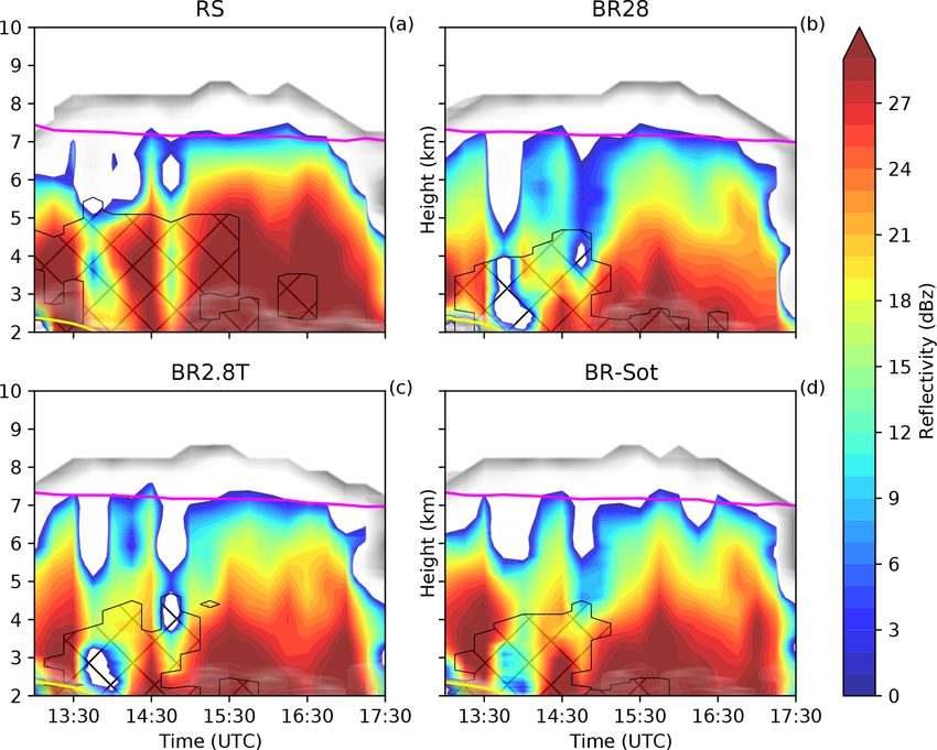
2346                                                                             Z. Dedekind et al.: Secondary Ice Production

tion of ice particles, secondary ice processes may occur. In       veyor belts (Houze and Medina, 2005; Gehring et al., 2020).
a narrow temperature range, −3 ≥ T ≥ −8 ◦ C, rime splinter-        These interactions are not limited to the accretional growth
ing (Hallett and Mossop, 1974) can occur when supercooled          of cloud hydrometeors but also include the fracturing of ice
cloud droplets collide with ice particles, freeze from the out-    particles in ice–ice collisions, enhancing SIP. Dedekind et al.
side in and shatter as a result of internal pressure buildup.      (2021) hypothesized that ice–graupel collisions are sensitive
Rime splintering has been studied extensively in models but        to the rate at which graupel forms, which is a function of the
has been shown to be inadequate to capture SIP in wintertime       ice particle size and the riming rate. In the Seifert and Be-
orographic MPCs (Henneberg et al., 2017; Dedekind et al.,          heng (2006) two-moment (2M) cloud microphysics scheme
2021; Georgakaki et al., 2022), producing ice number con-          used in this study, ice crystals or snow particles undergoing
centrations that are orders of magnitude less than observed.       riming can only be converted to graupel once they reach a
Ice–ice collisions have been more widely used in models in         size of 200 µm.
the last decade (Yano and Phillips, 2011; Phillips et al., 2017;      Remote sensing from weather radars is used to study
Sullivan et al., 2018; Hoarau et al., 2018; Sotiropoulou et al.,   snowfall microphysics and hydrometeor habit (e.g., shape,
2020; Zhao et al., 2021) since they were first studied in the      phase or hydrometeor type). Although radar observations do
laboratory about 4 decades ago (Vardiman, 1978; Takahashi          not provide direct information on SIP, a few studies lever-
et al., 1995). SIP as a result of ice–ice collisions was shown     aged the Doppler and/or dual-polarization capabilities of
to contribute significantly to the ice crystal number concen-      weather radars to identify the occurrence of SIP and to spec-
trations and thereby explain the discrepancy between mod-          ulate, case by case, on the possible mechanisms behind its
els and observations in the Arctic (Sotiropoulou et al., 2020;     origin. Two approaches can be found in the literature. Za-
Zhao et al., 2021), Antarctic (Sotiropoulou et al., 2021) and      wadzki et al. (2001), Oue et al. (2015) and Luke et al. (2021)
midlatitudes (Sullivan et al., 2018; Dedekind et al., 2021;        exploited Doppler spectra collected by vertically pointing
Georgakaki et al., 2022). The enhancement of smaller ice           radars to identify the appearance of secondary populations of
particles triggers an increase in the combined growth rates        particles at given altitudes or temperature levels. Other ap-
(reduced riming due to the smaller ice crystals but strong en-     proaches (Hogan et al., 2002; Andrić et al., 2013; Sinclair
hancement of deposition) of up to 33 %, resulting in larger        et al., 2016; Kumjian and Lombardo, 2017) focused on the
latent heat release and stronger updraft velocities (Dedekind      interpretation of the signature of dual-polarization variables
et al., 2021). When ice–ice collisions occur in wintertime         and their respective evolution over the vertical column of
orographic MPCs, the general tendency is for riming to de-         precipitation. This second approach, also used in this study,
crease. Hence, the depositional growth rate dominates the          leverages the fact that dual-polarization variables are com-
growth rates of ice particles. Due to the stronger updrafts,       plementary and impacted differently by changes in number,
ice particles are lofted to higher regions within the cloud re-    shape, size and density of hydrometeors. Additional informa-
ducing the local precipitation rates.                              tion (in situ data, models or a combination of more radars) is
   The impact of turbulence associated with baroclinic waves       typically needed to increase confidence in the retrievals col-
on cloud water and precipitation formation is well known           lected.
(Baumgartner and Reichel, 1975; Houze and Medina, 2005;               In this paper, we propose that the vertical wind shear asso-
Medina and Houze, 2015). Updrafts on the scale of ∼ 10 km          ciated with a cold front passage over the mountains of eastern
from baroclinic waves have properties of shear-induced tur-        Switzerland enhanced the formation of small and numerous
bulence, and it is these small cells of enhanced updraft and       oblate ice particles through ice–ice collisions. The ice–ice
turbulence that drive orographic precipitation (Medina and         collisions explain the peculiar signatures in the data collected
Houze, 2015). In regions associated with mountainous ter-          by a Doppler dual-polarization radar deployed in the region.
rain, strong shear layers at low levels approaching a bar-         We address the following questions:
rier were emphasized by Houze and Medina (2005) to set
up turbulence which in turn aids in precipitation growth             – Can these radar signatures be attributed to high ice crys-
(by accretion) on the windward side of a mountain. Med-                tal number concentrations linked to SIP other than rime
ina et al. (2005) showed in idealized simulations that a shear         splintering?
layer can develop as a response to flow over the terrain, by
which they concluded that this mechanism, in actual topog-           – By including ice–graupel collisions in the model, can
raphy, caused turbulent overturning which enhanced precipi-            we simulate the high ice crystal number concentrations
tation formation. In their simulation, the precipitation forma-        that were observed?
tion was linked to enhanced accretion (see also Medina and
Houze, 2015). The probability of interactions between cloud          – Was there a correlation between the vertical wind shear
hydrometeors, whether through riming and/or aggregation,               and SIP?
increases with increasing turbulence and aids in the rapid for-
mation of precipitation regardless of whether the turbulence         – How sensitive are SIP rates to the conversion rate of ice
is associated with orographic flow regimes or with warm con-           particles to graupel?

Atmos. Chem. Phys., 23, 2345–2364, 2023                                             https://doi.org/10.5194/acp-23-2345-2023
Z. Dedekind et al.: Secondary Ice Production                                                                                      2347

2     Methods                                                       exact location was 46.789◦ N, 9.843◦ E (see Sect. 2.1). MX-
                                                                    Pol is well suited for deployment in complex Alpine terrain
2.1    Weather radar and two-dimensional video                      or remote locations (e.g., Schneebeli et al., 2013; Grazioli
       disdrometer (2DVD)                                           et al., 2015a, 2017) and was operated from September 2009
                                                                    to July 2011. The radar was routinely scanning over the
The principle of dual-polarization for weather radars relies        valley of Davos in a sequence including pseudo-horizontal
on radars transmitting pulsed horizontally and vertically po-       scans (fixed elevation and variable azimuth) and 2D vertical
larized waves (Field et al., 2016). The waves interact with         cross sections (fixed azimuth scans with elevation ranging
precipitation, and by looking at the differences in power and       from 0 to 90◦ , known as range height indicator or RHI scans).
phase of the echoes in each polarization, information about         One RHI scan in particular, used as a data source of this
the orientation, size and number concentration (and phase)          study, was conducted every 5 min towards the NE, at an az-
of the hydrometeors being sampled can be retrieved. Hori-           imuth of 22◦ . Only observations collected at elevation angles
zontal (vertical) reflectivity ZH (ZV ) and differential reflec-    below 40◦ are used, in order to limit the effect of elevation
tivity ZDR are variables that exploit the power intensity of        dependencies on the polarimetric variables (Ryzhkov et al.,
the echoes. ZH [dBz] increases as particles get larger, denser      2005). MXPol provides single (ZH ) and dual-polarization
and/or more numerous. ZDR [dB] is the difference ZH − ZV            (ZDR , Kdp , ρHV ) measurements as well as Doppler data
and can be used to distinguish oblate particles (ZDR > 0)           which have proven useful in several snowfall microphysics
from prolate ones (ZDR < 0), while it has near-zero values          studies (e.g., Schneebeli et al., 2013; Grazioli et al., 2015a;
for spherical particles. In an environment where preferen-          Kumjian and Lombardo, 2017; Oue et al., 2021). Addition-
tially oriented anisotropic ice particles are dominant, ZDR         ally, retrieval algorithms adapted to polarimetric data allow
deviations from near-zero values are frequently observed            for estimated properties such as hydrometeor type (Grazioli
(Bader et al., 1987; Kumjian et al., 2014). When ice particles      et al., 2015b, as used in this work) or, under given assump-
form aggregates and become larger and less oblate, ZDR de-          tions, microphysical quantities such as ice crystal number
creases while ZH increases (Schneebeli et al., 2013; Kumjian        concentration Nt , median volume diameter D m or ice water
et al., 2014; Grazioli et al., 2015a). The backscattered power      content (IWC). The hydrometeor classification method dis-
is different for horizontal and vertical polarizations in the       criminates between three ice-phase dominant hydrometeor
presence of anisotropic particles, as is the propagation speed      types: individual ice crystals, aggregates and rimed particles.
of the waves.                                                          The microphysical quantities can be estimated from a
   The rate of change in phase shift between the horizontal         combination of ZH , ZDR , Kdp and the radar wavelength fol-
and vertical polarized echoes is expressed by the specific dif-     lowing Murphy et al. (2020):
ferential phase shift Kdp [◦ km−1 ]. This variable is comple-
mentary and not redundant; it is in fact not affected by the ab-                         Kdp λ
                                                                    IWC = 4 × 10⁻³         −1
                                                                                                   ,                               (1)
solute calibration of a radar and is less affected than ZDR by                        1 − Zdr
the eventual presence of large isotropic particles within the
                                                                                                                Zdp

sampling volume. For instance, local Kdp enhancements dur-          log10 (Nt ) = 0.1ZH − 2 log10                       − 1.11,    (2)
                                                                                                                Kdp λ
ing snowfall have been documented (Schneebeli et al., 2013;                                     0.5
Bechini et al., 2013) and in some cases been associated with                             Zdp
                                                                    D m = −0.1 + 2                      .                          (3)
SIP (e.g., Andrić et al., 2013; Grazioli et al., 2015a; Sinclair                        Kdp λ
et al., 2016). Grazioli et al. (2015a) suggested in a case study
that an increase of Kdp can be due to very large number con-        In these equations, IWC is expressed in [g m−3 ], Nt in [L−1 ]
centrations of rimed anisotropic ice crystals resulting from        and D m in [mm]. λ is the radar wavelength in [mm], Zdr =
ice–ice collisions. A recent study (von Terzi et al., 2022) sug-    100.1 ZDR is the differential reflectivity in linear units and
gested that the Kdp enhancement was due to a combination            Zdp = 100.1 ZH − 100.1 ZV is the reflectivity difference in lin-
of secondary ice production and an appropriate temperature          ear units [mm6 m−3 ]. More details about the derivations of
range T ≈ −15 ◦ C (where growth of planar crystals by va-           these equation can be found in Ryzhkov and Zrnic (2019)
por deposition, dendrites in particular, is maximized). Den-        and Murphy et al. (2020). The main assumptions are the fol-
drites have very low densities, favor aggregation (hence the        lowing:
increase of ZH below Kdp peaks) and can easily fracture on
impact with other ice particles.                                      – The equations are derived assuming to be in the
   An X-band dual-polarization mobile Doppler weather                   Rayleigh regime, which may not be fulfilled for the X-
radar (MXPol) of the École Polytechnique Fédérale de Lau-               band wavelength and large hydrometeors.
sanne Environmental Remote Sensing Laboratory (EPFL-
LTE) was set up at 2133 m above mean sea level (a.m.s.l.)             – The density and the size of the hydrometeors are as-
on a ski slope overseeing the valley of Davos (Schneebeli               sumed to be inversely proportional, which is not ful-
et al., 2013) from the southern side as shown in Fig. 1. Its            filled for hail.

https://doi.org/10.5194/acp-23-2345-2023                                            Atmos. Chem. Phys., 23, 2345–2364, 2023
2348                                                                             Z. Dedekind et al.: Secondary Ice Production

The retrievals have shown to be most reliable at T < −10 ◦ C,
for low riming degrees and in regions where the Kdp and ZDR
signals are not close to 0. As recognized by Murphy et al.
(2020), the errors may be large, and in situ validation efforts
are needed to refine these techniques. As a final caveat, the
equations developed theoretically are in practice very sensi-
tive to the accuracy of the polarimetric variables, which can
be very noisy. Kdp in particular is an estimated variable af-
fected by mean errors on the order of 30 % (Grazioli et al.,
2014a).
   An additional ground-based source of information for this
event is provided by a two-dimensional video disdrometer,
2DVD (for more information about this instrument at this lo-
cation, see Grazioli et al., 2014b), which was deployed on
the opposite side of the Davos valley with respect to MXPol
(46.830◦ N, 9.810◦ E; 2543 m a.m.s.l.). The 2DVD measures
the size and fall velocity of hydrometeors captured within
its measurement area of 11 cm × 11 cm. The 2DVD is used           Figure 1. Overview of the model orography and the instrument lo-
in this study as ground reference to quantify the number con-     cation setup. The parallelogram (dashed black lines) is the domain
centration of snowflakes (larger than 0.2 mm in terms of max-     of the flow-oriented vertical cross-section analysis in Sect. 3.1 fol-
imum dimension, according to the sensitivity of the instru-       lowing the direction of the dual-polarized Doppler radar MXPol
ment itself) at a temporal resolution of 5 min.                   (red dot located at 46.789◦ N, 9.843◦ E) data. The blue box is the
                                                                  domain used for analysis in Sect. 3.2 and 3.3. The red triangle is the
                                                                  location of the ground-based video disdrometer.
2.2     Model setup

2.2.1    Spatial and temporal resolution                          ciated with simulating atmospheric processes in mountain-
The Consortium for Small-scale Modeling (COSMO; Bal-              ous terrain, three cross sections were interpolated from the
dauf et al., 2011) non-hydrostatic model, version 5.4.1b, was     model output (only the outer two cross sections are shown in
used for this case study. COSMO has been used to study            Fig. 1). Each cross section, of which one cross section cuts
wintertime (Lohmann et al., 2016; Henneberg et al., 2017;         more or less through the location of the radar, is separated
Dedekind et al., 2021) and summertime (Dedekind, 2021;            by 1 km which is similar to the model resolution. The direc-
Eirund et al., 2021) orographic MPCs in the Swiss Alps. The       tion of each of the cross sections is similar to the direction of
model domain roughly covers a region of 500 km × 600 km           the generated RHI cross section from the weather radar. The
(44.5 to 49.5◦ N and 4 to 13◦ E) at a horizontal grid spacing     three cross sections are then averaged and compared to the
of 1.1 km × 1.1 km (Fig. 1). A height-based hybrid smoothed       radar data. To generate the Hovmöller diagrams, we further
level vertical coordinate system (Schär et al., 2002) with 80     took the mean along the length of the cross section for both
levels is used and stretched from the surface to 22 km. For       the simulations and the radar data.
this study, we simulate the cold front passage between 11:00
and 18:00 UTC and analyze the results between 13:00 and           2.2.2   Cloud microphysics scheme
18:00 UTC on 26 March 2010. COSMO is forced with initial
and hourly boundary conditions from reanalysis data at a hor-     We use a detailed two-moment bulk cloud microphysics
izontal resolution of 7 km × 7 km, supplied by MeteoSwiss.        scheme within COSMO with six hydrometeor categories,
The model time step is 4 s with an output frequency every         including cloud droplets, rain, ice, snow, graupel and hail
15 min.                                                           (Seifert and Beheng, 2006). The 2M scheme has been used
   Simulations were conducted including several SIP pro-          extensively to study the evolution, lifetime, persistence and
cesses, which consisted of ice–graupel collisions (as thor-       aerosol–cloud interactions of MPCs (Seifert et al., 2006; Bal-
oughly discussed in Sect. 2.2.2 below) and a control sim-         dauf et al., 2011; Lohmann et al., 2016; Possner et al., 2017;
ulation, referred to as the rime-splintering (RS) simulation,     Henneberg, 2017; Glassmeier and Lohmann, 2018; Sullivan
where only rime splintering was active. For each of these se-     et al., 2018; Eirund et al., 2019, 2021). We refer to ice par-
tups, five ensemble simulations are conducted by perturbing       ticles as any combination of the hail, graupel, snow or ice
the initial temperature conditions at each grid point through     categories. Cloud droplet activation is based on an empirical
the model domain with unbiased Gaussian noise at a zero           activation spectrum which depends on the cloud-base vertical
mean and a standard deviation of 0.01 ◦ C (Selz and Craig,        velocity and the prescribed number concentration of cloud
2015; Keil et al., 2019). To account for the uncertainty asso-    condensation nuclei (Seifert and Beheng, 2006). The appli-

Atmos. Chem. Phys., 23, 2345–2364, 2023                                              https://doi.org/10.5194/acp-23-2345-2023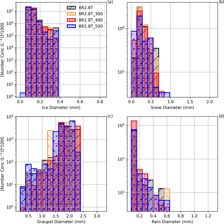
Z. Dedekind et al.: Secondary Ice Production                                                                                        2349

Table 1. Sensitivity settings for the collisional-breakup (BR) pa-       ligram of rime is used in the rime-splintering parameteriza-
rameterization. The conversion rate (conv) is the size (in µm) at        tion. Another SIP process, collisional breakup, was added to
which rimed ice crystals or snowflakes are converted to graupel,         COSMO and tested in several studies (Sullivan et al., 2018;
α is the scale factor, FBR is the fragments generated, and γBR is        Dedekind et al., 2021). Generally, collisional breakup refers
the decay rate of fragment number at warmer temperatures. When           to the collision of any two frozen hydrometeors with differ-
γBR = 5, as used in the Takahashi parameterization (Sullivan et al.,
                                                                         ent densities in which the collisional kinetic energy is suffi-
2018), then T is included in the simulation name. The bold num-
bers represent the sensitivity simulations pertaining to the different
                                                                         cient that the collisional impact causes shattering. Here, col-
conversion sizes of 300, 400 and 500 µm.                                 lisional breakup is when either ice or snow particles collide
                                                                         with graupel and fracture. This can increase the number of
       conv       α    FBR /α     γBR = 5          γBR = 2.5             ice particles at temperatures warmer than −21 ◦ C. Almost
                                                                         no empirical constraint – apart from Takahashi et al. (1995),
       200        1        280    BR-Sot                                 who used collisions between hail-sized particles – exists for
       200       10         28                     BR28                  the efficiency of any form of collisional breakup. The colli-
       200      100         2.8   BR2.8T
                                                                         sional kinetic energy and the density between hydrometeors
       300      100        2.8    BR2.8T_300
       400      100        2.8    BR2.8T_400
                                                                         are important parameters for this efficiency. In this study of
       500      100        2.8    BR2.8T_500                             the heavy snowfall event during which high Kdp values were
                                                                         recorded, we use the parameterizations for ice–graupel colli-
                                                                         sional breakup (BR) from Dedekind et al. (2021, BR28 and
                                                                         BR2.8T) and Sotiropoulou et al. (2021, BR-Sot) in COSMO
cation is appropriate in atmospheric models with a horizontal            in different forms:
grid size and time resolution of 1x ≤ 1 km and 1t < 10 s,
                                                                                FBR
                                                                                    (T − 252)1.2 exp −(T − 252)/γBR

respectively. The warm-phase autoconversion process from                 ℵBR =
Seifert and Beheng (2001) was updated with the collision                         α
efficiencies from Pinsky et al. (2001) and also takes into ac-           for BR28 (FBR , α, γBR ) = (280, 10, 2.5),                   (4)
count the decrease in terminal velocity associated with an in-                  FBR
                                                                                    (T − 252)1.2 exp −(T − 252)/γBR

                                                                         ℵBR =
crease in air density. A better approximation of the collision                   α
rate between hydrometeors was also introduced by Seifert                 for BR2.8T (FBR , α, γBR ) = (280, 100, 5),                  (5)
and Beheng (2006), which makes use of the Wisner approx-
                                                                                                                     D
imation (Wisner et al., 1972).                                           ℵBR = FBR (T − 252)1.2 exp −(T − 252/γBR )

   Primary production of ice occurs via homogeneous and                                                               D0
heterogeneous nucleation pathways. Homogeneous freez-                    for BR-Sot (FBR , D 0 , γBR ) = (280, 0.02, 5),              (6)
ing of cloud droplets, parameterized from the homogeneous
freezing rates of Cotton and Field (2002), is calculated for             where ℵBR is the number of fragments generated per colli-
0 > T ≥ −50 ◦ C. At −38 ◦ C most cloud droplets will freeze              sion, α is the scale factor, FBR is the leading coefficient, T is
given the enhanced homogeneous nucleation rates at colder                the temperature in kelvin, γBR is the decay rate of the frag-
temperatures. As a lower bound, the homogeneous freezing                 ment number at warmer temperatures, D is the diameter of
of all cloud droplets occurs at T = −50 ◦ C. The homoge-                 particles undergoing fracturing and D 0 is the diameter of the
neous nucleation of solution droplets, typically associated              hail particles used in Takahashi et al. (1995) (Table 1). Be-
with cirrus cloud formation, follows Kärcher et al. (2006).              cause of the inconsistency between the hail particles and their
Here, the number density and size of nucleated ice crystals              corresponding fall velocity used in Takahashi et al. (1995),
are determined by the vertical wind speed, temperature and               which is described in more detail in Dedekind et al. (2021),
pre-existing cloud ice. Heterogeneous nucleation is empiri-              all the parameterizations (Eqs. 4, 5 and 6) have scaling fac-
cally derived, which depends on the chemical composition                 tors. Equations (4) and (5) were applied in Dedekind et al.
and surface area of multiple species of aerosols, namely, or-            (2021) for the BR28 and BR2.8T simulations, respectively.
ganics, soot and dust (Phillips et al., 2008).                           Equation (4) is scaled by α = 10 and has a slower decay rate
   Secondary ice production through rime splintering, which              of fragment number at warmer temperatures represented by
is widely used in numerical weather prediction models, is                γBR = 2.5, and Eq. (5) is scaled by 100 while using the same
the only process that is included in the standard version of             decay rate of fragment numbers of γBR = 5 as used in Sul-
COSMO (Blyth and Latham, 1997; Ovtchinnikov and Ko-                      livan et al. (2018), which was derived from Takahashi et al.
gan, 2000; Phillips et al., 2006; Milbrandt and Morrison,                (1995) (Table 1). Equation (6), for the BR-Sot simulation,
2016; Phillips et al., 2017). In COSMO, rime splintering oc-             was applied in Sotiropoulou et al. (2021). They used a scal-
curs at −3 ≥ T ≥ −8 ◦ C (Hallett and Mossop, 1974) when                  ing parameter, D/D 0 , that was applied to the breakup param-
supercooled droplets and rain drops (Dc,r ≥ 25 µm) collide               eterization from Sullivan et al. (2018) where D 0 = 0.02 m.
with ice hydrometeors (Di,s,g ≥ 100 µm) (e.g., Seifert and                  Similar to Dedekind (2021), the ice crystal number con-
Beheng, 2006). A default value of 350 fragments per mil-                 centration (ICNC) in COSMO is limited to 2000 L−1 . Fur-

https://doi.org/10.5194/acp-23-2345-2023                                                 Atmos. Chem. Phys., 23, 2345–2364, 2023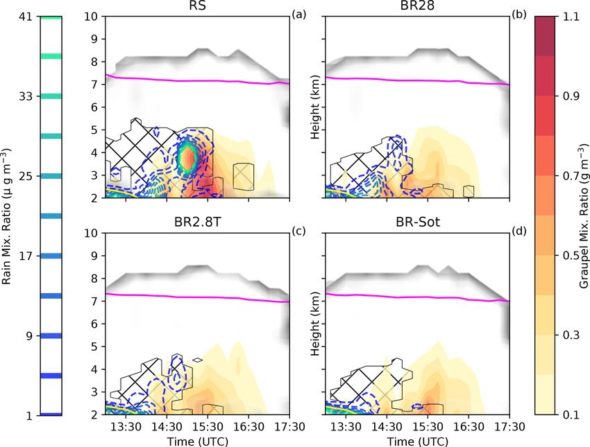
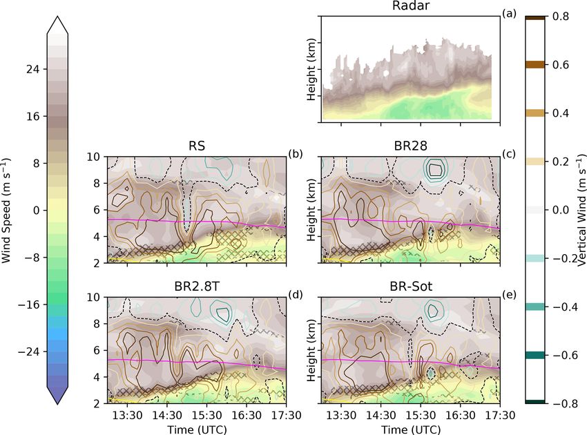
2350                                                                                   Z. Dedekind et al.: Secondary Ice Production

Figure 2. Hovmöller diagrams of wind speed and vertical velocity for panels (a) Doppler radar, (b) RS, (c) BR28, (d) BR2.8T and (e) BR-
Sot between 13:00 and 17:30 UTC. The filled contours denote wind blowing towards (blue and green) and away (white and brown) from the
radar, respectively. The pink line is the −21 ◦ C isotherm. At warmer temperatures collisional breakup occurs. Hatching denotes the region
where the air layer is dynamically unstable, determined by a bulk Richardson number of less than 0.25.

thermore, Dedekind (2021) concluded that the conversion                tween the SIP rate and cloud properties (e.g., Dawe and
rate from ice crystals or snow to graupel, which is a func-            Austin, 2013). For this purpose, a 10 km × 10 km region was
tion of the riming rate of ice crystals or snow with raindrops,        selected and masked by the levels in which SIP occurred
may contribute to enhanced collisional breakup (Seifert et al.,        (T > −21 ◦ C, blue box in Fig. 1) from 15:15 to 16:30 UTC.
2006). In Eq. (70) of Seifert and Beheng (2006), they specify          This resulted in the 16 121 data points for which an expres-
that ice and snow crystals can only be converted to graupel            sion from Hacine-Gharbi et al. (2013) was used for finding
once they reach D i,s ≥ 500 µm. However, in the current ver-           the optimal number of bins (17 bins in our case) to estimate
sion of the 2M scheme (as used in this study), ice and snow            the MI for continuous random variables.
crystals are converted to graupel already once they exceed
D i,s ≥ 200 µm. Therefore, earlier graupel formation is pro-
moted in the current version, which should lead to enhanced            3     Results
SIP though ice–graupel collisions. To test the model’s sensi-
tivity to these different thresholds for graupel formation, we         3.1    The case study
set up sensitivity studies with graupel formation at D i,s ≥           A synoptic system passed over Switzerland on
300, 400 and 500 µm to understand how the conversion rate              26 March 2010, during which we analyzed the evolu-
impacts SIP processes. To accomplish this, we change the               tion of a cold front from 13:00 to 17:30 UTC with intense
ice category conversion size requirement, D i,s , during rim-          precipitation from 15:00 to 17:30 UTC. Furthermore, the
ing from 200 µm (BR2.8T) to 300 µm (BR2.8T_300), 400 µm                cold front was associated with a surface temperature drop
(BR2.8T_400) or lastly 500 µm (BR2.8T_500) (Table 1). The              of ∼ 7 ◦ C (Fig. S1 in the Supplement), a southwesterly
results of these sensitivity simulations can be found in Ap-           wind flow at higher altitudes, vertical wind shear closer
pendix C.                                                              to the surface below 4 km a.m.s.l. and the development
   To investigate the impact of vertical wind shear and up-            of peculiar polarimetric radar signatures. In particular,
draft on SIP, the probability density functions (PDFs) for the         Kdp reached values around 1.5◦ km−1 at certain height
variables from the collisional-breakup simulations are ana-            levels, and towards the end of the event it was exceeding
lyzed. Furthermore, the joint PDFs are calculated along with           2◦ km−1 (Fig. 3a). A statistical analysis of Kdp in snowfall
the mutual information (MI, Shannon and Weaver, 1949)                  conducted with this radar and in this location over a long
score, which quantifies the strengths of dependencies be-              observation period (Schneebeli et al., 2013) showed that the

Atmos. Chem. Phys., 23, 2345–2364, 2023                                                   https://doi.org/10.5194/acp-23-2345-2023
Z. Dedekind et al.: Secondary Ice Production                                                                                 2351

80th percentile of Kdp at every height level is lower than         The vertical evolution of Kdp and ZDR is similar, with a peak
0.5◦ km−1 . Considering that the distribution of Kdp is very       observed about 4 km a.m.s.l., which is 1 km above the peak in
skewed, values above 1◦ km−1 in snow can be considered             ZH (Fig. 5b). The large and colocated values of ZDR and Kdp
unusually large.                                                   suggest that a large population of oblate and rimed particles,
   Wind shear, observed by the dual-polarization Doppler           without a significant presence of large isotropic hydromete-
radar, was visible between 2 and 5 km a.m.s.l. (Fig. 2a). The      ors, was present.
wind velocity at lower altitudes shifted from southerly to            Later, during the event (Fig. 3) the peak of ZDR was
northerly, which was captured in all simulations, albeit not       more often above the peak of Kdp , suggesting that the pop-
as prominent as the observations (Figs. 2b–e). The wind            ulation of particles in the areas of enhanced Kdp also in-
shear and the associated updrafts may have contributed to          cluded larger isotropic aggregates. The occurrence of peaks
an enhanced SIP rate between 3 and 5 km in the collisional-        in polarimetric variables at certain heights above ground
breakup simulations (Fig. 2c–e). Here, the bulk Richardson         (Kdp in particular) has been observed during intense snowfall
number, which is a ratio of the buoyant energy to shear-           events (e.g., Kennedy and Rutledge, 2011; Schneebeli et al.,
kinetic energy, is determined to assess the dynamic stability      2013; Grazioli et al., 2015a). The Kdp enhancement in partic-
of the air layer. An air layer becomes turbulent if the Richard-   ular has often been observed near the −15 ◦ C isotherm and
son number is less than the critical Richardson number of          has been interpreted as the signature of enhanced dendritic
0.25 (e.g., Stull, 2016). Figure 2b–e shows where the air layer    growth (Kennedy and Rutledge, 2011; Bechini et al., 2013) in
was turbulent with enhanced interactions between ice parti-        combination with secondary ice production (von Terzi et al.,
cles that could have caused enhanced ice–graupel collisions.       2022). Dendrites are prone to aggregation; therefore, the Kdp
Regions of enhanced updraft, where hydrometeors can grow           peak disappears (and ZH increases) as particles approach the
to larger sizes, were mostly seen immediately above the tur-       ground level.
bulent layer.
   The subzero temperature in the region of enhanced Kdp           3.2.2   Modeled and measured cloud properties
was warmer than −21 ◦ C, which is in the temperature range
favorable for ice–graupel collisions (Takahashi et al., 1995).     Throughout the vertical profile below 6 km at 15:30 UTC,
We thus hypothesize that the in situ cloud conditions together     the ice crystal number concentration was at least an order
with the vertical wind shear could have triggered higher sec-      of magnitude larger than expected from the RS simulation
ondary ice production rates that can be reflected in radar         with a SIP rate in excess of 20 L−1 s−1 (Fig. 6). In both
measurements, as Kdp is a possible indicator of high number        Figs. 6 and S2 the observed ice crystal number concentration
concentrations of oblate hydrometeors in the radar sampling        recorded by the disdrometer (∼ 20 L−1 ) was remarkably well
volume (Kennedy and Rutledge, 2011; Bechini et al., 2013;          represented at the surface by the BR2.8T and BR-Sot simu-
Grazioli et al., 2015a; von Terzi et al., 2022).                   lations (similar results are shown in Dedekind et al., 2021).
                                                                   The ice crystal and snow number concentrations were orders
                                                                   of magnitudes larger for D i < 0.4 mm and D s < 0.8 mm, re-
3.2     Simulated vs. observed radar reflectivity                  spectively, compared to the RS simulation (Fig. 7a and b).
3.2.1    Model and Doppler radar comparison                           During the late stage of the snowfall event, at 17:00 UTC,
                                                                   the replenishment of graupel diminished rapidly (Figs. 8 and
Horizontal reflectivity ZH is used to compare the model to         S2c), causing a substantial reduction in the SIP rate (Fig. S2).
the observations throughout the cloud and to analyze the im-       Less collisional breakup allowed the ice and snow crys-
pact of secondary ice production on the simulated radar re-        tals to grow to larger sizes, D i ∼ 1.2 mm and D s ∼ 3.3 mm,
flectivity. During the early afternoon, the median of ZH re-       respectively, primarily through deposition and/or aggrega-
mained mostly below 20 dBz. At around 15:15 UTC larger             tion (Fig. S3a and b). A lower ZDR is consistent with less
ice hydrometeors were present (either as a result of en-           anisotropic particles produced by aggregation and/or riming.
hanced aggregation or depositional growth) between 4 and           However, the enhanced concentration of oblate particles (in-
6 km a.m.s.l., which then started to sediment (Fig. 3c and d).     crease in Kdp ) was in contrast to the simulations, showing
A peak in ZH at 3 km a.m.s.l. was observed in the fall streaks     a reduction in cloud content as the cloud began to dissipate
when the cloud droplets rimed onto the sedimenting ice hy-         earlier than in the observations. None of the simulations were
drometeors. The RS simulation overestimated ZH by at least         able to describe the high ice particle formation event that was
8 dBz throughout the vertical profile at 15:30 UTC, while all      most likely triggered through ice–ice collisions of aggregates
the collisional-breakup simulations captured ZH more accu-         of dendrites given the favorable temperature range.
rately, especially between 3 and 5 km a.m.s.l. (Figs. 4 and
5a). The radar-derived hydrometeor classification showed           3.2.3   Microphysical explanations
that much of the ice hydrometeor growth occurred through
aggregation and riming. At 15:30 UTC, very high median             ZH was significantly overestimated by the RS simulation be-
Kdp > 1◦ km−1 and ZDR > 1 dB were observed (Fig. 5b).              tween 13:00 and 17:30 UTC, which most likely was a result

https://doi.org/10.5194/acp-23-2345-2023                                           Atmos. Chem. Phys., 23, 2345–2364, 2023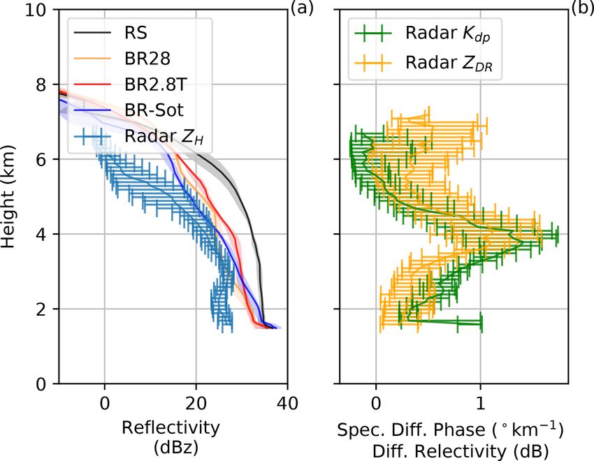
2352                                                                                         Z. Dedekind et al.: Secondary Ice Production

Figure 3. Hovmöller diagrams of the (a) spectral differential phase (Kdp ), the (b) differential reflectivity (ZDR ), (c) the horizontal reflectivity
(ZH ) and (d) the hydrometeor class categories derived from the Doppler radar between 13:00 and 17:30 UTC. The gray and black lines in
panels (a) and (b) are where both Kdp and ZDR are larger than 0.5 and 1, respectively.

of the following chain of events. (1) Insufficient droplets of                  When collisional breakup was allowed to occur in the
size 25 µm (Fig. 7d), within the narrow temperature range                    BR28, BR2.8T and BR-Sot simulations, the ice and snow
(−3 ≥ T ≥ −8 ◦ C), led to a limitation in ice particle growth                crystals did not have time to grow as large compared to the
by riming and therefore limited rime splintering (Fig. 6b).                  ice and snow crystals in the RS simulation. The smaller ice
(2) Because rime splintering was not that active, typical for                particles were associated with a reduced ZH which compared
wintertime MPCs (e.g., Henneberg et al., 2017; Dedekind                      better to the observations than the RS simulations.
et al., 2021), the ice and snow crystals grew mainly by de-                     Comparing the collisional-breakup simulations showed
positional growth and aggregation. (3) The ice and snow                      that the BR28 simulation still generated 8 times more
crystal size distributions widened substantially (Figs. 7a, b                ice particles than the BR2.8T and BR-Sot simulations at
and S3a, b). Both of these categories had number concentra-                  4 km a.m.s.l. at T ≈ −15 ◦ C (Fig. 6b). At temperatures of
tions of less than 100 L−1 with particle diameters of up to                  −10 ◦ C (3 km a.m.s.l.), the SIP rate decreased rapidly from
0.8 and 5.1 mm, respectively, at 15:30 UTC. (4) The larger                   100 L−1 s−1 to almost 0 L−1 s−1 at the surface. The lower
ice and snow crystal diameters resulted in enhanced ZH .                     SIP rates (less ice–graupel collisions) compared to the
These observations are consistent with other times during                    BR2.8T and BR-Sot simulations had several implications:
the day which showed even larger-sized ice and snow crys-                    (1) ice crystals and snow particles had more time to grow
tals of 0.9 and 5.2 mm, respectively (Figs. S4a and S5a), as                 to larger sizes as seen in the wider particle size distributions
well as higher rain mass mixing ratios (e.g., Fig. 8a). There                (Fig. 7); (2) the number of ice hydrometeors was an order
were single grid points where snowflakes even reached di-                    of magnitude below (worst in the collisional-breakup simu-
ameters of 13 to 17 mm during the latter part of the day                     lations) the observed ground-based video disdrometer obser-
(not shown here). Additionally, excessive size sorting in the                vations of ∼ 20 L−1 (for particles less than 0.2 mm) at 15:30
model most likely contributed to the overestimation in ZH .                  and 17:00 UTC (Figs. 6a and S2c); and (3) interestingly, the
Size sorting typically occurs within the sedimentation param-                simulated ZH compared slightly better with the radar obser-
eterization of 2M schemes in regions of vertical wind shear                  vations, although the ice hydrometeors were overestimated
or updraft cores (Milbrandt and McTaggart-Cowan, 2010;                       (Figs. 5a, 6a, S2c and S2d). Because the BR2.8T and BR-Sot
Kumjian and Ryzhkov, 2012). All these factors contributed                    simulations showed similar results, which were better than
to the RS simulation overestimating ZH compared to the ob-                   the BR28 simulation, only the BR2.8T simulation is used in
servations (Fig. 5a).                                                        the next section to link the simulated wind shear to SIP.

Atmos. Chem. Phys., 23, 2345–2364, 2023                                                          https://doi.org/10.5194/acp-23-2345-2023
Z. Dedekind et al.: Secondary Ice Production                                                                                          2353

Figure 4. Hovmöller diagrams of the simulated reflectively for panels (a) RS, (b) BR28, (c) BR2.8T and (d) BR-Sot between 13:00 and
17:30 UTC. The hatched area is defined as the MPC where the cloud droplet mass concentration and ice mass concentration are greater
than 10 and 0.1 mg m−3 , respectively. The pink line is the homogeneous freezing line at −38 ◦ C, and the shaded gray area is the cloud area
fraction.

                                                                        3.3    Linking simulated wind shear to SIP

                                                                        In this section, the dependence of the SIP rate on wind pat-
                                                                        terns is examined over the region (blue box) depicted in
                                                                        Fig. 1 during three time periods: 13:00–14:15 UTC (early,
                                                                        Fig. S6), 14:30–15:45 UTC (middle, Fig. 9) and 16:00–
                                                                        17:15 UTC (late, Fig. S7). The early period was categorized
                                                                        with strong wind shear and a turbulent layer below 3 km
                                                                        (Fig. 2a–e). During the middle period, the turbulent layer ex-
                                                                        tended to 4 km during which graupel increased in the MPC.
                                                                        The late period was categorized by less wind shear, caus-
                                                                        ing the dissipation of the turbulent layer. The cloud entered
                                                                        a glaciated state during this time. We analyzed the middle
                                                                        period as it was the most important period, according to the
                                                                        model, in terms of SIP and is therefore shown in Fig. 9. Re-
                                                                        gions in which SIP did not occur (e.g., T < −21 ◦ C) were
                                                                        masked out for this analysis.
                                                                           A strong shift between the early and middle period in the
Figure 5. Vertical profiles of the (a) horizontal reflectivity (ZH ),   V-wind median and interquartile range occurred from 20.5 to
(b) specific differential phase (Kdp ) and differential reflectivity    −0.7 m s−1 and 6.6 to 21.3 m s−1 , respectively, compared to
(ZDR ). The solid lines are the mean, with shaded areas and error       the U wind (Table 2). In fact, the U wind had a small variabil-
bars showing the 10th and 90th percentiles for the model simula-        ity between the early and middle periods (Table 2). As the af-
tions and Doppler radar, respectively, at 15:30 UTC.                    ternoon progressed, the median of the strongest V-wind shear
                                                                        extended from near the surface at 14:30 to 5 km a.m.s.l. at
                                                                        16:30 UTC (Figs. 2 and 9). Updraft cells developed above
                                                                        this level of strong vertical wind shear between 10 and

https://doi.org/10.5194/acp-23-2345-2023                                                 Atmos. Chem. Phys., 23, 2345–2364, 2023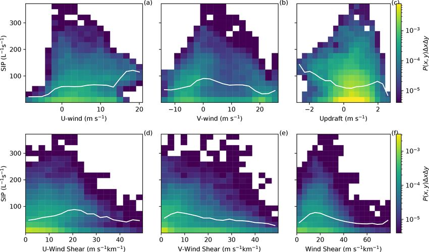
2354 Z. Dedekind et al.: Secondary Ice Production
PDF between the V wind and SIP (Fig. 10b) was highest
at this altitude. Here, an environment of stronger meridional
wind shear tends to coincide with the environment for high
secondary ice production (Fig. 10f and Table 2).
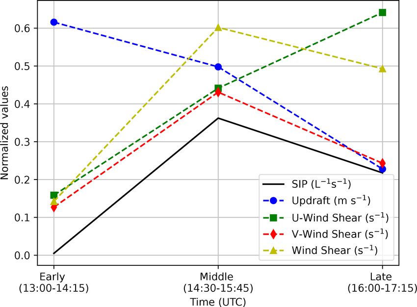
The contribution of the updraft velocity to SIP is not as
clear. The increase (early to middle period) and decrease
(middle to late period) of the median of the SIP rates poorly
co-varied with the U-wind shear or updraft compared to the
V-wind shear (Fig. 11).
To further highlight this role, we calculated the mutual
information shared between different sets of variables. The
mutual information (MI: I (X; Y )) between variables X and
Y was further analyzed for non-linear relationships (Shannon
and Weaver, 1949), where X ∈ [SIP rate] and Y ∈ [U wind,
V wind, updraft, U-wind shear, V-wind shear, wind shear].
I (X; Y )) of 0 bits means no information is shared between X
and Y ; therefore, Y cannot be inferred from X. (Further in-
formation about MI can be found in Appendix A and also in
Dawe and Austin (2013).) For instance, during the last period
the relationship of I (SIP rate; wind shear) weakened drasti-
cally to 0.021 bits to below the level of significance (Table 3)
compared to earlier periods. This was expected as the dimin-
ishing cloud liquid water caused a reduction in the riming
rates. Lower riming rates limited graupel formation which in
turn reduced ice–graupel collisions.
The significantly higher MI score between I (SIP rate;
wind shear) during the early and middle periods was a re-
sult of the strengthening of the northerly valley winds during
the early afternoon hours when the predominant wind aloft
was southwesterly (generating the dominant V-wind shear).
The development of the northerly winds could have been a
result of low-level blocking that generated the shear layer
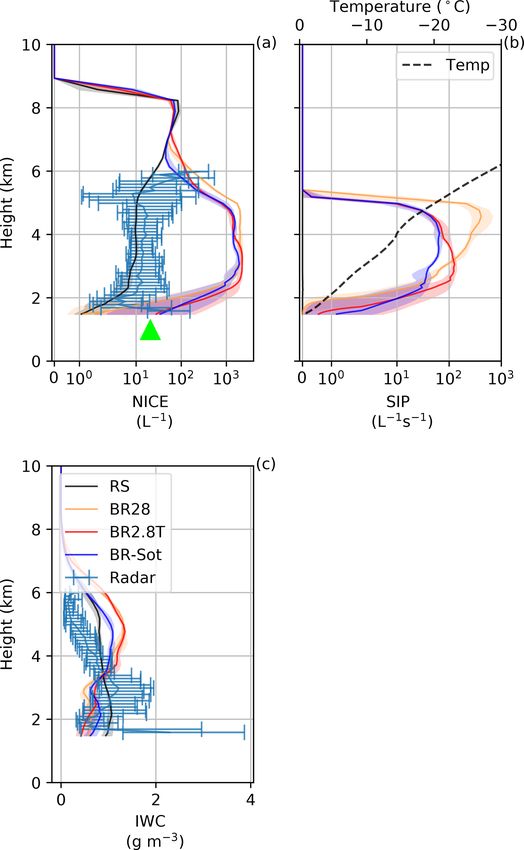
Figure 6. Vertical profiles for the (a) ice number concentration (Medina et al., 2005). The sharp change in the wind speed
(NICE), (b) secondary ice production (SIP) and (c) ice water con- and direction enhanced the turbulent overturning and there-
tent (IWC). The solid lines are the mean, with shaded areas and
fore promoted the riming of ice crystals and snow, leading
error bars showing the 10th and 90th percentiles for the model
simulations and Doppler radar, respectively, at 15:30 UTC. The
to the formation of graupel which in turn enhanced the SIP
green triangle is the 2DVD surface observations for hydrometeors rates. The higher MI score between I (SIP rate; wind shear)
D > 0.2 mm. implies there is a stronger relationship between wind shear
and SIP than the other variables analyzed here.
20 m s−1 km−1 . Our observation is consistent with Houze
and Medina (2005) and Medina and Houze (2015), who 4 Conclusions
also showed that updraft cells occurred at times and loca-
tions where the shear was strongest (>∼ 10 m s−1 km−1 ). A cold front passage on 26 March 2010, over the Swiss Alps,
During the middle time period, the variability in the V- associated with strong vertical wind shear and intense po-
wind shear was the largest with an interquartile range of larimetric signatures was observed with a dual-polarization
16.3 m s−1 km−1 , which coincided with the highest SIP rate Doppler weather radar deployed at Davos. This study inves-
(Fig. 9d and Table 2). The joint probability density functions tigates the role of vertical wind shear on the rate of SIP by
(PDFs) (P (SIP rate, V-wind shear)) illustrate that the correla- making simulations of wintertime orographic MPCs with a
tion median between the V-wind shear and SIP rate peaked at non-hydrostatic, limited-area model, COSMO, which has a
9 m s−1 km−1 and 80 L−1 s−1 (Fig. 10e). This peak coincided two-moment bulk microphysics scheme with six hydrome-
with the region where the wind shifted from southwesterly teor categories, as well as two additional parameterizations
to northerly (along the valley) between the early and middle for ice–graupel collisions (e.g., Sotiropoulou et al., 2020;
periods. This shift was a result of the change in the V-wind Dedekind, 2021) based on Takahashi et al. (1995). To con-
speed from negative to positive at 2.9 km a.m.s.l. The joint clude, our main findings can be summarized as follows:
Atmos. Chem. Phys., 23, 2345–2364, 2023 https://doi.org/10.5194/acp-23-2345-2023Z. Dedekind et al.: Secondary Ice Production 2355
Figure 7. Particle size distribution for panels (a) ice, (b) snow, (c) graupel and (d) raindrops for all the simulations at 15:30 UTC.
– Large values of Kdp > 1◦ km−1 suggest that a large pop- the disdrometer observations of ∼ 20 L−1 (considering
ulation of oblate particles was present, most likely origi- the 0.2 mm observation limit) at 15:30 and 17:00 UTC.
nating from ice–ice collisions, at 4 km a.m.s.l. This level
coincided with the −15 ◦ C isotherm. At −15 ◦ C den- – During the middle period, 14:30–15:45 UTC, the V-
dritic growth is very fast, causing low-density dendrites wind shear increased by 60 %, causing conditions fa-
to fracture and aggregate. At this time, ZDR was also vorable for accretion and leading to enhanced graupel
positive, indicating that large isotropic particles were formation and SIP in the region favorable for SIP.
less present. At lower altitudes, ZH increased while Kdp
(and ZDR ) decreased, suggesting aggregation and/or – Another time period with high Kdp but low ZDR was
riming were occurring. observed at 17:00 UTC, which was not captured by the
breakup simulations as the graupel mixing ratio was de-
– The rime-splintering simulations overestimated ZH pleted. The breakup parameterization does not include
throughout the vertical profile and underestimated the ice–ice collisions and relies only on graupel as the col-
disdrometers’ number concentration of hydrometeors at liding species. At this time, the radar signatures sug-
the surface. Both shortcomings could be explained by gested that collisions of dendrites caused the formation
omission of ice–graupel collisions. of small oblate particles (increasing Kdp ) but also the
formation of a few, larger, isotropic aggregates (decreas-
– The breakup simulations (BR28, BR2.8T and BR-Sot) ing ZDR ).
caused narrower ice crystal and snow distributions (en-
hanced number concentrations of smaller ice particles), – The mutual information between the SIP rate and other
resulting in a better representation of ZH . The enhanced variables like vertical wind shear and updraft velocity
number concentrations of ice particles meant that these suggested that the SIP rate is best predicted by the over-
simulations, in particular BR2.8T and BR-Sot, captured all wind shear.
https://doi.org/10.5194/acp-23-2345-2023 Atmos. Chem. Phys., 23, 2345–2364, 20232356 Z. Dedekind et al.: Secondary Ice Production Figure 8. Hovmöller diagrams of graupel and rain mixing ratio for panels (a) RS, (b) BR28, (c) BR2.8T and (d) BR-Sot between 13:00 and 17:30 UTC. The hatched area is defined as the MPC where the cloud droplet mass concentration and ice mass concentration are greater than 10 and 0.1 mg m−3 , respectively. The pink line is the homogeneous freezing line at −38 ◦ C, and the shaded gray area is the cloud area fraction. Figure 9. Probability density functions of different variables (P (x)) from the BR2.8T simulation from all model levels (top row) and at each model level (bottom row) for (a, e) secondary ice production (SIP) rate, (b, f) wind shear, (c, g) U-wind shear and (d, h) V-wind shear between 14:30–15:45 UTC. The solid and dashed white lines are the horizontal 50th percentile and the 25th and 75th percentiles, respectively, of each variable over the 10 km×10 km domain. Atmos. Chem. Phys., 23, 2345–2364, 2023 https://doi.org/10.5194/acp-23-2345-2023
Z. Dedekind et al.: Secondary Ice Production                                                                                           2357

Figure 10. Joint probability density function multiplied by bin area (P (x, y)1x1y) for the model output of SIP versus (a) U wind,
(b) V wind, (c) updraft, (d) U-wind shear, (e) V-wind shear and (f) wind shear for the BR2.8T simulation. White lines are the 50th per-
centile as a function of the x-axis variable.

Table 2. The 25th, 50th and 75th percentiles and the interquartile range (IQR) between the 10th and 90th percentiles of the vertical profiles
for the BR2.8T simulations.

                        Time (UTC)      Variable                        25th perc.   50th perc.    75th perc.   IQR
                        13:00–14:15     SIP rate (L−1 s−1 )                   0.0           0.4          3.5     3.4
                                        U wind (m s−1 )                       3.9           7.9         11.3     7.4
                                        V wind (m s−1 )                      15.9          20.5         22.5     6.6
                                        Wind speed (m s−1 )                  16.3          22.9         24.8     8.5
                                        Updraft (m s−1 )                      0.2           0.6          1.0     0.8
                                        U-wind shear (m s−1 km−1 )            2.0           4.3          7.4     5.5
                                        V-wind shear (m s−1 km−1 )            1.6           3.9         10.7     9.0
                                        Wind shear (m s−1 km−1 )              4.1           7.1         14.8    10.7
                        14:30–15:45     SIP rate (L−1 s−1 )                   4.7         28.5          78.7    73.9
                                        U wind (m s−1 )                       0.8          4.2           8.6     7.8
                                        V wind (m s−1 )                      −5.5         −0.7          15.8    21.3
                                        Wind speed (m s−1 )                   6.5         10.3          17.3    10.8
                                        Updraft (m s−1 )                      0.1          0.5           0.9     0.8
                                        U-wind shear (m s−1 km−1 )            4.1          8.4          13.9     9.8
                                        V-wind shear (m s−1 km−1 )            3.4          9.4          19.7    16.3
                                        Wind shear (m s−1 km−1 )              8.6         16.8          25.2    16.6
                        16:00–17:15     SIP rate (L−1 s−1 )                   0.7         17.2          53.2    52.5
                                        U wind (m s−1 )                       5.3         10.4          15.4    10.2
                                        V wind (m s−1 )                      −2.2         −0.2           3.7     6.0
                                        Wind speed (m s−1 )                   7.4         12.8          16.6     9.2
                                        Updraft (m s−1 )                     −0.0          0.2           0.5     0.5
                                        U-wind shear (m s−1 km−1 )            5.9         11.3          16.5    10.6
                                        V-wind shear (m s−1 km−1 )            3.1          6.1           9.8     6.8
                                        Wind shear (m s−1 km−1 )             10.3         14.5          19.6     9.3

https://doi.org/10.5194/acp-23-2345-2023                                                  Atmos. Chem. Phys., 23, 2345–2364, 2023
2358 Z. Dedekind et al.: Secondary Ice Production
Turbulent overturning, whether it is associated with baro-
clinic waves (Gehring et al., 2020) or low-level blocking
(Medina et al., 2005; Houze and Medina, 2005; Medina and
Houze, 2015), has been shown to play an important role in
accreting hydrometeors to form precipitation. Here, we con-
sidered that the interactions of ice hydrometeors can lead
to ice–graupel collisions, causing enhanced small ice frag-
ments, as opposed to only growing larger through aggre-
gation. These smaller fragments fall slower against updraft
and may decrease local precipitation rates, enhancing pre-
cipitation downstream of the flow (Dedekind et al., 2021).
Wind shear plays a significant role in ice–graupel collisions
and may even be more important when all ice–ice collisions
are considered in more physically robust collisional-breakup
parameterizations (Yano and Phillips, 2011; Phillips et al.,
Figure 11. Normalized median values of the PDFs of the variables 2017). By only considering ice–graupel collisions, we are
in Table 2 for the three different time periods for the BR2.8T simu- limited to mainly investigating collisional breakup in MPCs
lation. where riming can occur to form graupel. In the case where
a cloud becomes glaciated and graupel cannot form through
riming, our parameterization will not be able to simulate SIP,
Table 3. Mutual information between SIP rate and wind properties
which may still prove to be very important.
of the vertical profiles for the BR2.8T simulations. The significance
level is calculated by taking the maximum of 1000 Monte Carlo
simulations of mutual information between a random permutation Appendix A: Derivation of the simulated radar
of SIP rates and each variable. reflectivity
Time (UTC) Variable MI Sig. level
Here we briefly show the calculation of the simulated ZH
13:00–14:15 I(SIP rate;U wind) 0.025 0.009 (Appendix B, Seifert, 2002). Calculating ZH from the two-
I(SIP rate;V wind) 0.037 0.009 moment cloud microphysics scheme would not be possi-
I(SIP rate;wind speed) 0.029 0.009 ble without approximations and assumptions. The following
I(SIP rate;updraft) 0.027 0.009 relationship for the radar reflectivity of drops (Zw ), using
I(SIP rate;U-wind shear) 0.008 0.011 the Rayleigh approximation for the cross section of drops
I(SIP rate;V-wind shear) 0.015 0.011
(Eq. A1), results in
I(SIP rate;wind shear) 0.011 0.009
14:30–15:45 I(SIP rate;U wind) 0.091 0.018 Z∞
π 5 |Kw |2
I(SIP rate;V wind) 0.116 0.018 ηw = D 6 fw (D)dD, (A1)
I(SIP rate;wind speed) 0.112 0.018 λ4R
0
I(SIP rate;updraft) 0.035 0.018
I(SIP rate;U-wind shear) 0.039 0.022
where D is the particle diameter, λR is the wavelength of
I(SIP rate;V-wind shear) 0.043 0.021
radar radiation, ηw is the volumetric liquid water content,
I(SIP rate;wind shear) 0.048 0.015
fw (D) is the number density distribution function for liq-
16:00–17:15 I(SIP rate;U wind) 0.105 0.054 uid water and Kw2 = 0.93 is the dielectric constant of liquid
I(SIP rate;V wind) 0.117 0.054 water. The reflectivity factor for cloud water is given by the
I(SIP rate;wind speed) 0.103 0.054 following:
I(SIP rate;updraft) 0.095 0.054
I(SIP rate;U-wind shear) 0.014 0.067 Z∞
I(SIP rate;V-wind shear) 0.029 0.067 λ4R
Z̃w = ηw = D 6 fw (D)dD
I(SIP rate;wind shear) 0.021 0.055 π 5 |Kw |2
0
Z∞
6 2 6 2
= x 2 fw (x)dx = Zw , (A2)
π ρw π ρw
– The sensitivity of the ice–graupel simulations to the 0
conversion rate size restriction was measured using
the Kullback–Leibler divergence. The sensitivity sim- where ρw is the water density. Because of the backscatter
ulations were not sensitive to the conversion rate size behavior for the mass-equivalent diameter with regards to ρw
thresholds. and ρi (ice density), the same applies to graupel, which is
Atmos. Chem. Phys., 23, 2345–2364, 2023 https://doi.org/10.5194/acp-23-2345-2023Z. Dedekind et al.: Secondary Ice Production 2359
described as a spherical ice particle entropy of X subtracted from the entropy of X conditioned
on Y ):
Z∞
π 5 |Ki |2 6 2
ηg = x 2 fg (x)dx1 , (A3) I (X; Y ) = H (X) − H (X|Y ). (B3)
λ4R π ρi
0
MI describes, therefore, how different the joint distribution
where x is the particle mass, fg (x) is the number density of the pair (X, Y ) is from the distribution of X and Y . Com-
distribution function for graupel and Ki2 = 0.176 is the di- bining Eqs. (B1) and (B3) yields
electric constant of ice. The radar reflectivity factor for ice Z
particles (e.g., graupel) is given by the following:
I (X; Y ) = [P (x)ln(P (x)) − P (x, y)ln(P (x|y))]dxdy,
Z∞
λ4R |Ki |2 6 2 (B4)
Z̃g = ηg = x 2 fg (x)dx
π 5 |Kw |2 |Kw |2 π ρi
0 and because P (x|y) = P (x, y)/P (y), Eq. (B5) can be re-
2 duced to
|2
|Ki 6
= Zg . (A4)
|2
Z
|Kw π ρi P (x, y)
I (X; Y ) = − P (x, y)ln dxdy. (B5)
P (x)P (y)
For melting ice particles, however, Kw must be used instead
of Ki . In our study, the surface and in situ cloud temperatures The range of the MI is described as follows:
were below 0 ◦ C. More information on the reflectivity calcu-
lations for melting ice particles can be found in Seifert (2002, 0, if P (x, y) = P (x)P (y)
Appendix B). Finally, the radar reflectivity factor is given by
(X and Y are completely independent),
MI = (B6)
10
Zradar
H (X), if P (x, y) = P (x) = P (y)
dBZ = ln , (A5)
ln 10 mm6 m−3 (X and Y are perfectly correlated).
where Zradar is the sum of the reflectivity calculated for each
Appendix C: SIP sensitivity to conversion rates
individual cloud particle category (e.g., cloud drops, rain-
drops, ice crystals, snow crystals, graupel and hail): In this section the sensitivity of SIP to the rate of graupel
" # formation, which is dependent on ice or snow crystals being
6 2 ρw2 |Ki2 |
larger than a given size when riming occurs, is analyzed.
Zradar = Zc + Zr + 2 Zic + Zs + Zg . (A6)
π ρw ρi |Kw2 | Figure C1 shows the particle size distribution (PSD) for
the sensitivity studies during which the size restrictions are
Appendix B: Mutual Information modified, which could slow the conversion process of the
ice crystals and snow particles to graupel. The PSD over the
The entropy H of the variable x’s probability density func- cross section at 15:30 UTC showed little difference in the
tion P (x) is defined by Shannon and Weaver (1949) to be ice crystal number concentrations where we expected higher
Z ice crystal number concentration for BR2.8T and conse-
H = − P (x)ln(P (x))dx, (B1) quently higher snow number concentrations due to enhanced
aggregation (Fig. C1a and b). The largest differences from
where x is the information content of a single measurement the BR2.8T_300 simulation were in the form of enhanced
of P (x) = − ln P (x). The entropy is a measure of the amount snow (for diameters 0.14 < D s < 0.42 mm) and graupel
of information that is required to represent the PDF. From number concentrations (for diameters 1.2 < D g < 2.2 mm).
here, both the Kullback–Leibler divergence and the mutual However, at 15:30 UTC there is no clear signal beyond
information can be calculated. model variability, showing that the slower conversion rates
The Kullback–Leibler divergence, also known as the rela- to graupel affect the simulations (Fig. C1b and c). We
tive entropy, measures the distance between two probability compared the probability distributions of the total number
distributions, P (x) and Q(x), over a discrete random variable of ice hydrometeors (NISG, i.e., ice crystals, snow and
X. The Kullback–Leibler divergence is defined as follows: graupel), SIP rate, ice crystal and graupel number concen-
trations of the BR2.8T_500, BR2.8T_400 and BR2.8T_300
simulations, respectively, to that of the reference simulation,
Z
P (x)
DKL (P k Q) = P (x)ln dx. (B2) BR2.8T, between 14:15 and 15:45 UTC (Fig. 8b). We chose
Q(x)
this time period as the largest graupel concentrations were
The mutual information (MI) is a measure of the mutual de- present. The Kullback–Leibler divergence (DKL (P k Q)),
pendence between two random variables X and Y (e.g., the which measures how one probability distribution P is
https://doi.org/10.5194/acp-23-2345-2023 Atmos. Chem. Phys., 23, 2345–2364, 2023You can also read