Currents generated by the sea breeze in the southern Caspian Sea
←
→
Page content transcription
If your browser does not render page correctly, please read the page content below
Ocean Sci., 18, 675–692, 2022
https://doi.org/10.5194/os-18-675-2022
© Author(s) 2022. This work is distributed under
the Creative Commons Attribution 4.0 License.

Currents generated by the sea breeze in the southern Caspian Sea
Mina Masoud and Rich Pawlowicz
Department of Earth, Ocean and Atmospheric Sciences, University of British Columbia,
2207 Main Mall, Vancouver, BC, V6T 1Z4, Canada

Correspondence: Mina Masoud (mmasoud@eoas.ubc.ca)

Received: 9 June 2021 – Discussion started: 29 June 2021
Revised: 24 February 2022 – Accepted: 21 March 2022 – Published: 13 May 2022

Abstract. The sea breeze system is the dominant atmo-               Zhang et al., 2009; Sobarzo et al., 2010; Gallop et al., 2012).
spheric forcing at high frequency in the southern Caspian           These coastal currents can dominate the high-frequency vari-
Sea. Here, we describe and interpret current meter obser-           ability over continental shelves (DiMarco et al., 2000; Rip-
vations on the continental margins of the southern Caspian          peth et al., 2002; Hyder et al., 2002; Simpson et al., 2002).
from 2012 to 2013 to identify and characterize the water col-       However, it is often difficult to separate tidal, inertial, and
umn’s response to the sea breeze system. Time series anal-          sea breeze effects in the coastal ocean response, since the
ysis provides evidence for diurnal baroclinic current signals       timescales are very similar.
of O(0.02 m s−1 ) and surface height changes of O(0.03 m).             Recently, it was found that the variability of shelf cur-
A two-layer model, including interfacial and bottom friction,       rents in the southern Caspian Sea (Fig. 1a) is mostly dom-
is developed to further investigate the sea breeze response.        inated by coastally trapped waves with timescales of sev-
This model is able to reproduce the structure, amplitudes,          eral days or longer (Masoud et al., 2019) but a significant
and phases of observed diurnal current fluctuations, explain-       daily signal is also present. The Caspian Sea, about 1030 km
ing half of the variance in observational current response at       long and 310 km wide, is the largest enclosed basin in the
frequencies at 1 cpd and higher. The sea breeze response thus       world, and the southern coast, which is characterized by a
results in a “tide-like” daily cycle, which is actually linked to   shallow shelf of width 10–30 km with a deeper basin off-
the local forcing all along the southern Caspian coast.             shore, has a very persistent sea breeze pattern that is present
                                                                    through most of the year. Meteorological aspects of this pat-
                                                                    tern have been well-studied (Khoshhal, 1997; Azizi et al.,
                                                                    2010; Karimi et al., 2016), and analysis of a short current
1   Introduction                                                    record at one station suggested that this sea breeze was linked
                                                                    to high-frequency variations in water column currents (Ghaf-
Diurnal-period onshore to offshore wind variability is a per-       fari and Chegini, 2010). Further, since tides in the Caspian
sistent feature of many coastal areas, especially in tropical       Sea are very weak (Medvedev et al., 2016, 2017, 2020), it
and subtropical areas, but also in temperate zones (Sonu            is possible that most of the higher-frequency variations in
et al., 1973; Simpson, 1994; Steyn, 1998). Due to the smaller       coastal currents may be a response to the sea breeze system.
thermal heat capacity of land, it heats more rapidly in the day        Here, we take advantage of the strong and persistent sea
and cools more rapidly at night relative to the sea, resulting      breeze forcing in the southern Caspian Sea and the lack of
in land–sea thermal gradients with a daily cycle. This leads to     confounding tidal effects, as well as the availability of mea-
cross-shore pressure gradients which generate onshore to off-       sured current records at five well-separated locations along
shore wind flows, called sea breeze systems, with the same          the southern Caspian shelf obtained between late 2012 and
daily periodicity. The diurnal sea breeze system can have a         late 2013, to investigate the nature of a geophysical water
significant impact on the incident wave climate, nearshore          column response on a shelf to periodic sea breezes. We find
processes, and morphology in tropical and subtropical re-           that the water column response to the sea breeze is mea-
gions (Sonu et al., 1973; Masselink and Pattiaratchi, 2001).        surable and widespread, occurring over the entire southern
Coastal currents can also be generated (Hyder et al., 2002;

Published by Copernicus Publications on behalf of the European Geosciences Union.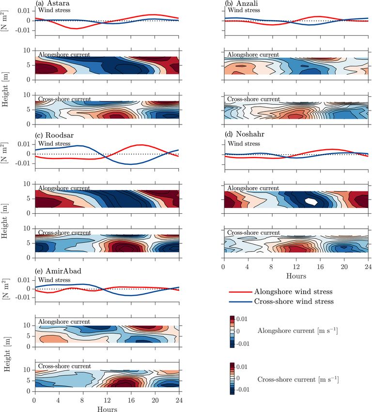
676                      M. Masoud and R. Pawlowicz: Currents generated by the sea breeze in the southern Caspian Sea

Figure 1. (a) Southern Caspian Sea with the location of current meter moorings. Topography above and below the levels of the Caspian is
derived from the ETOPO2 dataset (National Geophysical Data Center, 2001); the water level in the Caspian Sea is 28 m b.m.s.l. (below mean
sea level). (b) Wind roses for total winds at mooring locations (Anzali and Noshahr roses are shifted southwards for clarity). (c) Wind roses
for diurnal band-passed winds. Rings appear at 2 %, 4 %, and 6%.

Caspian shelf year-round. However, the coupling between                  the freshwater input (Alizadeh et al., 2008). The large-scale
the atmosphere and ocean is a strongly local phenomenon,                 stratification in the Caspian’s water column varies season-
with changes in the timing of the daily cycle of currents re-            ally, with warm salty (20–30 ◦ C, 12 PSU) waters in a rela-
sponding to changes in the timing of the cycle of winds di-              tively well-mixed layer about 40–100 m deep in summer and
rectly overhead, with no sign of propagation effects along-              fresher, less warm (10 ◦ C, 11 PSU) surface waters in winter
shore (unlike the case for lower-frequency current varia-                (Zaker et al., 2007) above more stratified waters at depth.
tions). Analytical solutions to a new coupled two-layer rotat-           However, even within this mixed layer there is often a weak
ing wind-driven shallow-water model are compared with ob-                stratification.
servations and show good agreement. Model dynamics also                     Atmospheric forcing governs the mostly cyclonic mean
explain the nature of the local response.                                circulation of the Caspian Sea, but winds are generally weak
                                                                         in the southern Caspian with mean speeds of only 3–4 m s−1 ;
1.1   The study area                                                     wind speeds are less than 5 m s−1 more than 90 % of the
                                                                         time (Kosarev, 2005). The occasional strong winds along the
                                                                         southern Caspian coast result in the formation of baroclinic
The Caspian Sea (Fig. 1a) is a terminal basin into which
                                                                         coastally trapped waves along the shelf edge (Masoud et al.,
rivers flow but water is only lost by evaporation; its surface is
                                                                         2019). These waves propagate from west to east at speeds
about 28 m below mean ocean level. Although the northern
                                                                         of 1–3 m s−1 and explain most of the variance in currents at
Caspian Sea is very shallow, with depths of less than 50 m,
                                                                         frequencies less than 1 cpd.
the southern part is characterized by a central region with
                                                                            The southern Caspian has a humid subtropical climate
depths of more than 800 m, bordered on the south and west
                                                                         characterized by warm summers and mild winters, and it
by a narrow shelf area (Fig. 1) extending 10–30 km offshore
                                                                         receives a significant amount of solar radiation (Kosarev,
to the 100 m isobath. Inshore of this is a coastal plain of vary-
                                                                         2005). At higher frequencies the sea breeze is then an im-
ing width, backed up by the Alborz mountains with heights
                                                                         portant phenomenon which exists throughout the year but is
of up to 5610 m. On the southeastern coast, the shelf extends
                                                                         most widespread in spring and summer months (Khoshhal,
offshore more than 100 km; the coastal plain there is simi-
                                                                         1997; Azizi et al., 2010; Ghaffari and Chegini, 2010; Karimi
larly flat and extends well inland.
                                                                         et al., 2016). A typical sea breeze in warm months is gen-
   Most of the fresh water enters from the Volga River in Rus-
                                                                         erated by solar radiation. However, in other months when
sia to the north. There are many small rivers on the south-
                                                                         the temperature gradient between the sea and land surfaces
ern (Iranian) coast, but together they supply only 5 % of

Ocean Sci., 18, 675–692, 2022                                                                  https://doi.org/10.5194/os-18-675-2022
M. Masoud and R. Pawlowicz: Currents generated by the sea breeze in the southern Caspian Sea                                            677

Table 1. Location, water depth, and distance to shore for all mooring locations. Also given is the direction of the principal axis of current
variations. The details of ADCPs located in deeper water are presented in the second column for Astara and Roodsar.

                  Station                             Astara         Anzali        Roodsar         Noshahr     AmirAbad
                  Longitude (◦ E)                 48.92    49.05      49.45     50.30     50.35       51.39         53.41
                  Latitude (◦ N)                  38.39    38.37      37.49     37.21     37.23       36.70         36.91
                  Distance from shore (km)          4.2     15.8        1.3       2.4       8.9         1.5           6.4
                  Water depth (m)                    10       31       10.5        10        32        10.5          13.7
                  Direction of major axis (◦ )   167.00   175.74      93.78    153.10    158.54       85.14          75.6

is low, other mechanisms, for example outflows from the Al-              gion, interpolated to the location of ADCP measurement sta-
borz mountains in winter known as Garmesh winds, can also                tions. The WRF model, described at length in Bohluly et al.
increase temperatures in the coastal plain, generating a sea             (2018), is configured with two nests. The 42 × 52 outer do-
breeze (Khoshhal, 1997; Karimi et al., 2016).                            main has a resolution of 0.3◦ , and the 94 × 124 inner domain
   A typical sea breeze cycle in the southern Caspian is char-           grid has a resolution of 0.1◦ . The 6-hourly ERA-Interim re-
acterized by onshore winds (the “sea breeze”) generally start-           analysis data from the European Centre for Medium-Range
ing more than 2 h after sunrise at around 9:00–noon (see,                Weather Forecasts (ECMWF) are used as initial and bound-
e.g., Azizi et al., 2010; Ghaffari and Chegini, 2010; Karimi             ary conditions. The model is run daily starting at 18:00 for
et al., 2016, all times referred to here are in local sum-               1.25 d with 6 h of spin-up time that is discarded. The accu-
mer time, which is known as Iran Daylight Time – IRDT                    racy of modeled winds has been evaluated by Bohluly et al.
– or UTC+4:30). The wind direction changes to offshore                   (2018) and Ghader et al. (2014). The latter compared model
(the “land breeze”) around 16:00–21:00. The maximum wind                 winds with a variety of observed wind products over the
speed of about 4 m s−1 occurs during the sea breeze between              Caspian Sea including one offshore buoy, three nearshore
noon and 16:00 after the time of maximum temperature gra-                buoys, and also data from the QuikSCAT satellite product.
dient between sea and land. The strongest and most frequent              Qualitative and quantitative assessment of these comparisons
sea breeze days occur in areas around AmirAbad and Anzali                showed that the simulated surface wind fields are in good
where the coastal plain is widest, and the fewest sea breeze             agreement with the observational data and QuikSCAT satel-
days are observed around Noshahr and Astara (Azizi et al.,               lite data. We also evaluated the accuracy of the WRF wind
2010; Karimi et al., 2016).                                              data ourselves by comparing with available wind buoy data
                                                                         at three locations during 2013 (the wind data are available
1.1.1   Data and data processing                                         mostly between May and September). The root mean square
                                                                         error (RMSE) between WRF wind and observed wind is
The wind and current meter datasets used here were fully de-             less than 0.1, 0.11, and 0.2 m s−1 at Anzali, Noshahr, and
scribed in Masoud et al. (2019), and only brief details are              AmirAbad, respectively. The wind stress is calculated from
given here. Over a period of about 16 months from late 2012              the 10 m elevation wind velocity from the WRF model us-
to early 2014, current velocity measurements using 600 kHz               ing drag coefficients from Large and Pond (1981). Since the
Nortek AWAC acoustic Doppler current profilers (ADCPs)                   WRF model is run on a daily cycle, the diurnal peaks in
were collected at five locations a few kilometers offshore in            the spectra that we describe later could be numerical arti-
depths of about 10 m over the southern Caspian shelf in suc-             facts. However, similarly strong diurnal peaks are observed
cessive monthly deployments (Fig. 1 and Table 1). Measure-               in spectra of observed wind from buoy data at Anzali and
ments for the period of December 2012 to December 2013,                  AmirAbad and from land stations located near Astara, An-
when spatial and temporal coverage was most complete, are                zali, Noshahr, and AmirAbad stations (not shown), so we be-
used here. More sparse information is also available at two              lieve the WRF outputs reflect real conditions. In addition, the
locations further offshore near the 30 m isobath at Astara and           daily analysis we perform in this paper starts at midnight, and
Roodsar. The instruments used collected data every 10 min                hence any systematic forecast-to-forecast step would occur at
with a vertical bin resolution of 0.5 m; the lowest useful bin,          figure boundaries.
which we use to show bottom currents, is 2 m above the bot-                 Finally, water levels in the southern Caspian are mea-
tom.                                                                     sured by tide gauges at Anzali (37.48◦ N, 49.46◦ E) and at
   Some local observations of surface winds are available at             AmirAbad (36.85◦ N, 53.37◦ E). For our purposes (to see
three stations (Anzali, Noshahr, and AmirAbad) out of our                daily variations) we subtract the daily mean from each day.
five stations during 2013, but even these data contain gaps.             This removes any biases resulting from a seasonal cycle with
So for consistency we use winds at 10 m above the water                  a range of about 0.4 m, as well as long-term trends.
surface, which are extracted from a Weather Research and
Forecasting (WRF) model configured for the Caspian Sea re-

https://doi.org/10.5194/os-18-675-2022                                                                    Ocean Sci., 18, 675–692, 2022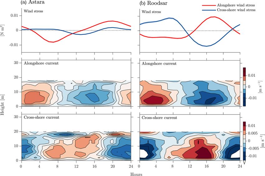
678                      M. Masoud and R. Pawlowicz: Currents generated by the sea breeze in the southern Caspian Sea

Table 2. Ratio of diurnal variance (band-passed filter with removing periods less than 6 h and more than 30 h) to high-frequency variance
(frequencies higher than 1 cpd) for alongshore and cross-shore wind stress and bottom current. Ratios are in percentage.

                             Station                     Astara    Anzali     Roodsar     Noshahr    AmirAbad
                             Alongshore wind stress      64.48     66.01       68.66       64.58        60.35
                             Cross-shore wind stress     64.76     65.76       69.73       69.02        72.20
                             Alongshore current          38.88     29.47       44.74       39.69        35.43
                             Cross-shore current         34.87     26.96       40.34       32.12        39.17

                                                                           2.1.1   Wind and current spectra

                                                                           Wind stress spectra have a narrow, statistically significant
                                                                           spectral peak at 1 cpd at all stations (Fig. 3a and c); it is
                                                                           strongest at Roodsar. There is both clockwise and anticlock-
                                                                           wise motion in diurnal frequencies, although the clockwise
                                                                           motion is stronger everywhere except at AmirAbad, con-
                                                                           sistent with the strong directionality of the daily wind rose
                                                                           there (Fig. 1c) and generally clockwise rotations elsewhere.
                                                                           Smaller spectral peaks also occur at the first harmonic of the
Figure 2. Definition of axes. Offshore direction is the positive           diurnal frequency (frequencies of ±2 cpd) at many stations
x axis; θ is the rotation angle between geographic and coastal axes.       and sometimes (e.g., at AmirAbad) at higher harmonics as
                                                                           well.
                                                                              Rotary spectra for bottom currents also have narrow, sta-
2     Results                                                              tistically significant peaks at 1 cpd and small peaks at the first
                                                                           harmonic frequencies (Fig. 3b and d). Spectra for wind and
2.1    Total and diurnal-period winds
                                                                           currents computed for each season rather than for the whole
Wind roses at our five study sites (Fig. 1b) show that winds               year (not shown here) also contain the 1 cpd peak. Although
are generally aligned along the coast, with maximum wind                   these peaks are always present they are largest in the sum-
speeds of about 10 m s−1 . However, if we separate out the di-             mer and spring. At frequencies higher than about 2 cpd, wind
urnal variability using a Butterworth fourth-order band-pass               stress spectra continue to slope downwards, whereas bottom
filter to remove periods less than 6 h and more than 30 h,                 current spectra begin to flatten. This suggests that the current
wind roses for this band-limited time series show mostly                   time series is mostly dominated by instrument white noise at
cross-shelf variation with speeds of up to 4 m s−1 at three sta-           these high frequencies. We shall then restrict our analysis to
tions. Diurnal winds at the other two (Astara and Noshahr)                 frequencies less than 2 cpd.
still have a significant alongshore component (Fig. 1c). As-                  Inertial frequencies, which at around 1.2 cpd at these lati-
tara is at the southern end of a large inland plain from                   tudes are well-separated from the diurnal frequency, are as-
which sea breezes are generated, so the sea breeze will align              sociated with a very weak peak in bottom currents at most
with the coast, and the coastal plain is also very narrow at               locations (Fig. 3d). Although we cannot separate the diur-
Noshahr, making it difficult to generate a large cross-shore               nal peak from any that might be associated with the domi-
wind.                                                                      nant diurnal tidal constituent (K1 ), there is clearly no visi-
    Subtracting the mean, the wind stress and current data are             ble peak at the frequency of the next most important diurnal
then rotated based on principal axes of the currents at 4 m to             constituent (O1 ) or at the frequency of the dominant semi-
align with the local bathymetry so that vectors are decom-                 diurnal constituent (M2 ), strongly suggesting that the diurnal
posed into alongshore and cross-shore components (Table 1,                 and semi-diurnal peaks represent a response to wind stress
Fig. 2). The diurnal wind stress represents about 60 %–72 %                forcing at those frequencies and not tidal variability.
of the high-frequency wind stress variability, depending on
                                                                           2.1.2   The sea breeze
location (Table 2), and the diurnal current variability repre-
sents about 27 %–45 % of the high-frequency current vari-
                                                                           In order to concentrate our attention on the sea breeze forcing
ability near the bottom.
                                                                           and response, ignoring the low-frequency variability which
                                                                           was discussed in Masoud et al. (2019), we will analyze only
                                                                           band-passed data (removing data with periods less than 6 h
                                                                           and more than 30 h) from now on. Examining a 4 d period
                                                                           typical of the summer (Fig. 4i), the daily cycle of the sea

Ocean Sci., 18, 675–692, 2022                                                                   https://doi.org/10.5194/os-18-675-2022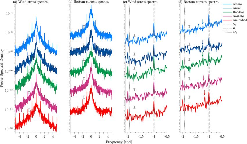
M. Masoud and R. Pawlowicz: Currents generated by the sea breeze in the southern Caspian Sea                                             679

Figure 3. Rotary power spectral density estimates of (a) wind stress and (b) bottom current at Astara, Anzali, Roodsar, Noshahr,
and AmirAbad stations using the Welch method. Successive spectra are offset downwards by 100 N m2 cpd−1 for wind stress and
100 m2 s−2 cpd−1 for currents. Negative and positive frequencies correspond to clockwise and counterclockwise rotation, respectively. The
grey error bars indicate 95% confidence intervals. (c) A magnification of the wind stress spectra for clockwise diurnal frequencies. (d) The
same for bottom currents. The arrows indicate the inertial frequency (at approximately 1.2 cpd) at each station, and other vertical grey lines
mark the location of the O1 (0.9295 cpd), K1 (1.0027 cpd), and M2 (1.9323 cpd) tidal frequencies.

breeze system is obvious, with onshore wind (the sea breeze)             Miller and Keim, 2003; Azorin-Molina and Chen, 2009). Ad-
in the late morning–early afternoon and offshore wind (the               ditionally, a rapid change in the intensity of wind is con-
land breeze) in the night–early morning. Winds rotate in the             sidered in some cases. Here, a sea breeze day is counted
clockwise direction. The daily cycle of band-passed wind di-             when (1) the wind direction during the day (from 10:00 to
rections for the whole study period demonstrates the predom-             23:00) is from the sea breeze direction (onshore) but the wind
inance of this daily change from onshore to offshore wind                overnight (from 23:00 to 10:00) is not from the same direc-
(Fig. 5) over the whole year. At all locations the wind blows            tion (greater than 60◦ wind direction difference) and (2) the
onshore in the early afternoon, starting at about 5 h after sun-         wind directions in the afternoon and morning are both from
rise (even as the time of sunrise varies over the year), and the         the sea breeze direction (onshore) but afternoon (noon to
onshore direction changes to offshore around sunset, remain-             23:00) wind speed is larger than wind speed in the morning
ing in that direction until late morning (Figs. 4i and 5).               (10:00 to noon).
   The diurnal bottom currents are slightly less consistent                 Using these selection criteria, about 220–280 sea breeze
from day to day (Fig. 4ii) but show an onshore current in                days occur in 2013 depending on the location, with a mean
the mornings and offshore currents in the evenings. Although             wind speed of 1.5 m s−1 (Fig. 6). The most are seen at Rood-
these currents also mostly turn clockwise, they are not in               sar (which also has the strongest winds) and the fewest at As-
phase with the winds, and their magnitude varies over the                tara. However, sea breeze activity is subject to a slight sea-
whole year (not shown) from less than 0.01 m s−1 to as much              sonal variability. In spring and summer (April–September),
as 0.2 m s−1 on occasion.                                                approximately 20–30 sea breeze days are experienced every
   More quantitatively, we count the number of sea breeze                month. However, closer to 10–25 sea breeze days occur per
days at all locations using a standard algorithm applied to              month in fall and winter seasons (October–March).
our band-passed datasets. In most selection methods for sea                 Water level measurements (Fig. 4iii) are available at
breeze days, the diurnal reversal of wind direction from off-            two locations. The daily range is about 0.1 m at both. At
shore to onshore is used as an identifier for a sea breeze               AmirAbad there is a “low” water level around noon and a
day (Masselink and Pattiaratchi, 2001; Furberg et al., 2002;             high water level a few hours after midnight. There is addi-

https://doi.org/10.5194/os-18-675-2022                                                                    Ocean Sci., 18, 675–692, 2022
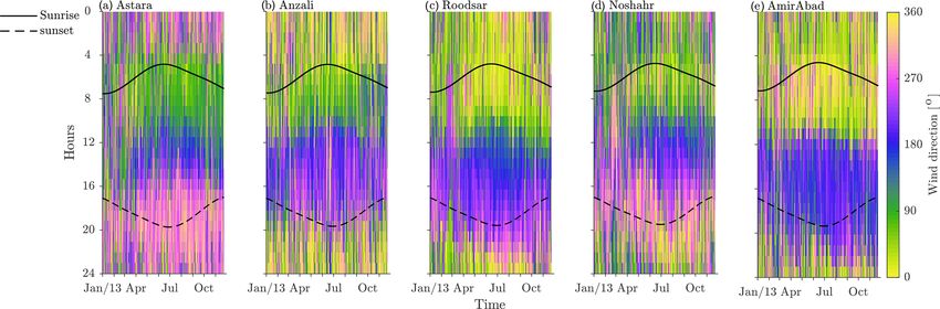
680                      M. Masoud and R. Pawlowicz: Currents generated by the sea breeze in the southern Caspian Sea

Figure 4. An example of summer daily variability from 21–25 July 2013. (i) Stick plot of hourly band-passed alongshore and cross-shore
winds at (a) Astara, (b) Anzali, (c) Roodsar, (d) Noshahr, and (e) AmirAbad. In this figure the coastline is horizontal with water above and
land below; positive upwards (positive y) winds in the morning are offshore, and negative downward (negative y) winds in the afternoon
are onshore. (ii) Stick plot of band-passed alongshore and cross-shore current at (a) Astara, (b) Anzali, (c) Roodsar, (d) Noshahr, and
(e) AmirAbad. (iii) Time series of sea level at (a) Anzali and (b) AmirAbad.

Figure 5. Wind direction at (a) Astara, (b) Anzali, (c) Roodsar, (d) Noshahr, and (e) AmirAbad. Angles increase clockwise from the offshore
direction so that a wind direction of 0/360◦ is pure offshore wind and 180◦ is pure onshore wind. The black solid and dashed lines are sunrise
time and sunset times, respectively (Beauducel, 2021).

Ocean Sci., 18, 675–692, 2022                                                                   https://doi.org/10.5194/os-18-675-2022
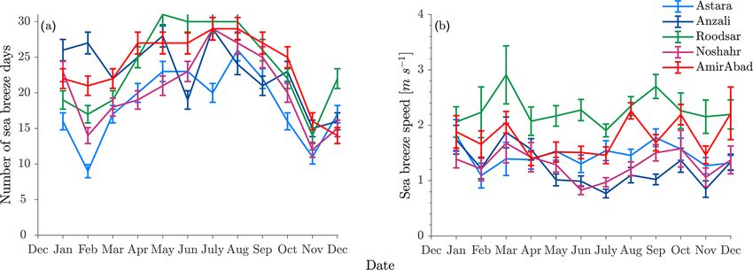
M. Masoud and R. Pawlowicz: Currents generated by the sea breeze in the southern Caspian Sea 681
Figure 6. (a) Number of sea breeze days and (b) sea breeze speed at Astara, Anzali, Roodsar, Noshahr, and AmirAbad stations for each
month from December 2012 to December 2013.
tionally a larger twice-a-day signal at Anzali. If we perform early as 9:00 at Noshahr but as late as 11:00 at Roodsar. The
a tidal harmonic analysis using T_Tide (Pawlowicz et al., transition back to offshore flow occurs at 16:00 at Noshahr
2002), we find M2 tidal amplitudes of 0.02 and 0.007 m for and Astara but as late as 23:00 at Roodsar and AmirAbad.
Anzali and AmirAbad stations, respectively. O1 amplitudes In the water column, the average diurnal cycle is similarly
are below the noise level, but S1 amplitudes, at 0.01 and uniform in its patterns at all locations, although the magni-
0.03 m for Anzali and AmirAbad, respectively, are signif- tude and exact timing of the cycle also vary from place to
icantly larger than their close neighbors P1 and K1 . S2 is place (Fig. 7). The cross-shore currents are almost entirely
also substantial. However, Medvedev et al. (2016), examin- baroclinic, with a node at a height above bottom of around
ing water level records in the central Caspian, suggest that the 6 to 7.7 m, a short distance above the middle of the water
anomalously large S1 and S2 constituents actually represent column (Fig. 7iii). Although we do not have measurements
“radiational” tides, probably resulting from the sea breeze. close to the bottom or surface due to limitations imposed by
The narrowness of these spectral peaks is then a result of the the ADCP design, it seems likely that this pattern consists of
extremely consistent sea breeze pattern over the whole year. the first baroclinic mode and that surface currents are coher-
ent with, but even larger than, those seen in the topmost bin
2.1.3 The mean diurnal cycle for which reasonable averages can be obtained. After mid-
night, there is an offshore flow in the surface layer, appar-
ently matching the offshore wind stress, and onshore flow at
Now we consider an “average” day. Although the annual
the bottom layer. An opposite pattern with an onshore flow in
changes in sunrise and sunset times result in a slight annual
the surface layer (and an onshore wind stress) and offshore
modulation in the timing of the sea breeze (Fig. 5), we ig-
flow at the bottom layer can be observed during daylight
nore this variation and average by hour of the day over the
hours. The magnitude of the average cycle is O(0.01 m s−1 ),
whole year. We also processed the data using only the de-
which is largest at Roodsar and Astara and smaller at the
duced “sea breeze” days, but find the smaller number of days
other three locations. Oscillation peaks, as well as peaks in
in the mean gave more variable results than averaging over
the offshore wind stress, occur slightly later at Roodsar and
the whole year; the sea breeze day selection algorithm ap-
AmirAbad relative to the other stations. These delays do not
pears to be overly conservative.
consistently trend eastwards or westwards and hence do not
The resulting time series of daily wind stress (Fig. 7) again
suggest alongshore propagation of wave-like features.
shows the same general pattern at all stations, but demon-
The alongshore cycle is also quite similar at all stations
strates a little more clearly how the magnitude of the signal,
(Fig. 7). Here, however, a noticeable barotropic flow can be
and the relative strengths of cross-shore and alongshore wind
seen, in addition to a baroclinic pattern. Current maximums
stresses, varies from place. Alongshore winds are to the right
and minimums of O(0.01 m s−1 ) near the bottom lag those
in the morning and to the left (when facing offshore) in the
at the surface by about 1/4 wave period so that they reach
afternoon and evening. These winds are strongest at Roodsar
a maximum while surface values approach zero (and vice
and weakest at Anzali. The daily cycle is not a pure sinusoid
versa). In the diurnal alongshore current pattern, there is a
but contains distortions associated with higher harmonics.
negative (rightward) flow in the daytime and positive (left-
These are greatest at AmirAbad, consistent with the appear-
ward) flow in the nighttime.
ance of wind spectra (Fig. 3). In addition, there are more sub-
The stronger winds at Roodsar and Astara are corre-
tle differences in the timing of peaks and transitions. For ex-
lated with stronger currents, and weaker winds at Anzali
ample, the transition from offshore to onshore flow occurs as
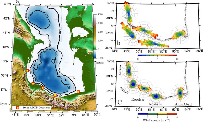
https://doi.org/10.5194/os-18-675-2022 Ocean Sci., 18, 675–692, 2022682 M. Masoud and R. Pawlowicz: Currents generated by the sea breeze in the southern Caspian Sea Figure 7. The 24 h averaged daily cycle of band-passed alongshore and cross-shore wind stress (first panel), as well as the alongshore current (second panel) and cross-shore current (third panel) at (a) Astara, (b) Anzali, (c) Roodsar, (d) Noshahr, and (e) AmirAbad stations from December 2012 to December 2013. The current data are band-passed and then averaged by hours; we remove values from bins that are too close to the surface and (at AmirAbad) bins with unstable averages. and Noshahr are associated with weaker currents. The tim- also located further offshore at the 31 and 32 m isobath (Ta- ing of changes in the direction of winds and the timing of ble 1). Although no useful data were returned from the upper changes in the direction of currents, which do vary slightly half of the water column there, the daily cycles of currents in from location to location, are also linked; locations with the lower half (Fig. 8) are similar in direction, magnitude, and later peaks and zero crossings in wind stress time series also timing to those seen at the bottom in the shallower locations, have later peaks and zero crossings in current time series. and there also weak indications at the shallowest depth for There is therefore a high (local) correlation between the sea which reliable measurements can be obtained that an upper breeze system and the diurnal currents all along the southern layer is present with flows similar to the upper layer flow in Caspian coast. shallower waters. Thus, daily oscillations in both surface and In addition to the moorings at depths of ∼ 10 m, two ad- bottom waters, with similar pattern and timing, are probably ditional current meter moorings at Astara and Roodsar were present in the water column over wide areas of the shelf. Ocean Sci., 18, 675–692, 2022 https://doi.org/10.5194/os-18-675-2022
M. Masoud and R. Pawlowicz: Currents generated by the sea breeze in the southern Caspian Sea                                         683

Figure 8. The 24 h averaged daily cycle of band-passed alongshore wind stress and cross-shore wind stress (first panel), as well as the
alongshore current (second panel) and cross-shore current (third panel) for (a) Astara at 31 m and (b) Roodsar at 32 m (Table 1).

2.2   Theoretical water column response to the sea
      breeze                                                                                  τ (x)    r
                                                                      u1t − f v1 = −gη1x +          −      (u1 − u2 ) − Ru1 ,        (1)
                                                                                             ρH1 H1
To further understand the linkages between the diurnal sur-
face wind stress and the diurnal currents, we now attempt                           τ (y)   r
                                                                      v1t + f u1 =        −     (v1 − v2 ) − Rv1 ,                   (2)
to model the dynamics. Instead of following the depth-                              ρH1 H1
dependent “oscillating Ekman layer” approach of Craig                 (η1 − η2 )t + H1 u1x = 0,                                      (3)
(1989b) with a vertical eddy viscosity coupled to a barotropic
mode, which has been used by many authors, we restrict our-           and the lower layer of undisturbed depth H2 ≈ 6.5 m is gov-
selves to a mathematically simpler coupled two-layer system,          erned by
as suggested by our observations, for which analytical solu-                                                 r
tions are more straightforward to obtain.                             u2t − f v2 = −g[(1 − ε)η1 + εη2 ]x −      (u2 − u1 ) − Ru2 ,
                                                                                                             H2
   Thus, consider a linearized two-layer shallow-water model                                                                         (4)
on the semi-infinite plane bounded by a coastline on the                              r
y axis, with the positive x axis pointed offshore (Fig. 2) into       v2t + f u2 = −    (v2 − v1 ) − Rv2 ,                           (5)
                                                                                     H2
shelf waters of depth HT ≈ 10 m (numerical values for these
                                                                      η2t + H2 u2x = 0,                                              (6)
and other parameters are presented here without comment to
justify the mathematical development; we shall discuss their          with g the gravitational acceleration, (ui , vi ) velocities and
origin in the next section). Since we are considering a local         Hi layer depths for the upper (i = 1) and lower (i = 2) layers,
response over scales of the shelf width, we will filter out long      ε = (ρ2 − ρ1 )/ρ ≈ 2 × 10⁻⁴ (with ρi layer densities and ρ a
shelf waves (which in any case are not suggested by our ob-           reference density), and τ (x) and τ (y) applied wind stresses in
servations at daily frequencies) by assuming negligible vari-         the offshore and alongshore directions. In this set of equa-
ation in the alongshore direction, but we retain the possibility      tions, r is an interfacial friction, and R represents a bottom
of an alongshore wind stress. Also, since the mooring loca-           friction, both characterized by their timescales r −1 and R −1 ,
tions are well inshore of the shelf break and energy that prop-       respectively. We (somewhat inconsistently) include R in both
agates across the shelf break will not return, we can neglect         the upper and lower layer equations since this allows us
the increase in depth past the shelf break. The upper layer of        to completely separate the baroclinic and barotropic modes
undisturbed depth H1 ≈ 3.5–6 m is then governed by                    next. The equations for each layer are fully coupled by the

https://doi.org/10.5194/os-18-675-2022                                                               Ocean Sci., 18, 675–692, 2022
684 M. Masoud and R. Pawlowicz: Currents generated by the sea breeze in the southern Caspian Sea
appearance of the interface height η2 in both, as well as by the associated surface height changes), and high-frequency
the interfacial friction; wind stress affects only the surface interface
p displacements travel with an intrinsic speed of
layer. The coastline boundary condition is that u1 = u2 = 0 gεH 0 ≈ 0.07 m s−1 , much slower than for the barotropic
at x = 0. mode. More importantly, the friction for the baroclinic mode
Using procedures described in Sect. 16 of LeBlond and must be greater than or equal to that affecting the barotropic
Mysak (1981), these six coupled equations can be approxi- mode, but the forcing stress is also larger (see changes in de-
mately separated into two independent sets of three equations nominator of the wind stress terms).
each when ε
1. A barotropic mode for which Now, we wish to find the response of this system
to a known diurnally oscillating (and possibly rotating)
H1 + H2 wind stress. Fortunately, the equations governing both the
u1 = u2 and η1 = η2 , (7)
H1 barotropic and baroclinic modes are almost identical, albeit
implying that the two interfaces move together in the same with coefficients whose numerical values are different so that
direction with about the same magnitude and that currents the same analytic solution can easily be adapted for either.
are the same from top to bottom, is then governed by the For simplicity, let us consider a canonical set of equations as
following equations. follows.
ut − f v = −gηx + T (x) − r 0 u
τ (x)
ut − f v = −gηx + − Ru (8) vt + f u = T (y) − r 0 v
ρHT
τ (y) ηt + H ux = 0 (21)
vt + f u = − Rv (9)
ρHT Now assume that both alongshore and cross-shore wind
ηt + HT ux = 0 (10) stress vectors decay offshore with a length scale α −1 (≈
100 km) and are oscillatory with a daily-frequency ω mod-
where eled by the real part of
H1 u 1 + H2 u 2 (x) (y)
u≈ (11) T (x) = T0 e−αx−iωt and T (y) = T0 e−αx−iωt (22)
HT
η ≈ η1 (12) (x) (y)
for constants T0 and T0 .
HT ≈ H1 + H2 (13) We look for solutions that vanish as x −→ ∞. The total
solution is made of a particular solution to the forced prob-
Thus, this mode is mostly linked to sea surface height lem and a homogeneous solution to the unforced equations,
variations.
√ The intrinsic speed of high-frequency waves is which are added together to match the coastal boundary con-
gHT ≈ 10 m s−1 . dition. For the particular solution, we guess that u, v, and
In addition, there is also a separate baroclinic mode for η will also decay offshore with a scale α −1 and oscillate with
which a frequency ω:
H1 H2
u2 = − u1 and η1 = −ε η2 , (14) u = Up e−αx−iωt , v = Vp e−αx−iωt , η = Np e−αx−iωt , (23)
H2 H1 + H2
where it is implicit in this approach that we take only the
governed by real part of the final (complex) solution. A nondimensional
τ (x) r decay scale, σ = r 0 /ω (which we will find to be ≈ 0 for the
ut − f v = −gεηx + − + R u, (15) barotropic mode but ∼ 1 for the baroclinic mode), is defined
ρH1 H0
to consider frictional effects. The particular solution then sat-
τ (y) r
isfies
vt + f u = − + R v, (16)
ρH1 H0 (x)
− iω(1 + iσ )Up − f Vp = gαNp + T0 , (24)
ηt + H 0 ux = 0, (17)
(y)
− iω(1 + iσ )Vp + f Up = T0 , (25)
where
− iωNp − H αUp = 0, (26)
u ≈ u1 − u2 , (18) whose solution for horizontal velocities in matrix form is
η ≈ −η2 , (19) " #
1 iω(1 + iσ ) −f
H1 H2 Up
= · 2
n o
H0 ≈ , (20) Vp β f iω (1 + iσ ) + gHω2α
H1 + H2
" #
(x)
which implies that for this mode, velocity shear is linked to T0
· (y) , (27)
mid-water interface depth changes (which are far larger than T0
Ocean Sci., 18, 675–692, 2022 https://doi.org/10.5194/os-18-675-2022M. Masoud and R. Pawlowicz: Currents generated by the sea breeze in the southern Caspian Sea 685
where Note that in the baroclinic case, the expressions within the
braces will be dominated by the first term (except very near
β = ω2 (1 + iσ )2 − f 2 + gH α 2 (1 + iσ ), (28) the coast) so that the baroclinic current magnitude and phase
response will be similar everywhere on the shelf and will be
with the height linked to offshore velocities through of similar magnitude in both the along and cross-shore direc-
iH α tions. However, for the barotropic case, the similarity of α
Np = Up . (29) and I m{k} means that the cross-shore barotropic current re-
ω
sponse will be very small and may be much smaller than the
For the homogeneous problem, a wave-like solution is alongshore barotropic response. These conclusions about rel-
considered: ative amplitudes are in general accord with our observations
(Fig. 8).
u = U eikx−iωt , v = V eikx−iωt , η = N eikx−iωt , (30) From our observations, we have both cross-shore and
alongshore winds of similar magnitude, and in this case it
leading to a dispersion relation of
becomes difficult to generalize further about the relationships
ω2 (1 + iσ ) − f 2 /(1 + iσ ) between currents and the wind stress. Thus, for further anal-
k2 = (31) ysis we now try and tune the predicted response to our ob-
gH
servations by first matching the measured daily wind cycle
(x) (y)
as well as (i.e., finding T0 and T0 specifically for each location) and
then, by taking the offshore distances and layer heights from
fU
V = (32) our observations, adjusting the offshore decay scale α −1 and
iω(1 + iσ ) frictions R and r as global parameters to match the observa-
and tions.
kH U 2.2.1 Fitting of model to data
N= . (33)
ω
Fitting sinusoids with a period of 1 d to the daily wind stress
Although in the inviscid limit there are free waves prop- (y) (y)
time series to estimate T0 and T0 for each location is
agating offshore (real k) for frequencies above the inertial
straightforward (Fig. 9i), as these time series are clearly dom-
frequency and evanescent waves (i.e., imaginary k with so-
inated by the daily variations with only a small amount of en-
lutions decaying exponentially in x) at lower frequencies,
ergy in the higher harmonics, as we have seen earlier (Fig. 3).
as will be the case in the Caspian, once friction is signifi-
However, the lack of ADCP data near the surface results in
cant then k will be complex. Here we have decay scales of
some difficulty in separating the barotropic and baroclinic
I m{k}−1 ≈ 200 km for the barotropic mode and around 1 km
modes in the water column observations. The layer interface
for the baroclinic mode. We can also (by combining with
is evident from the baroclinic response in Fig. 7 at about 6–
Eq. 28) write
7.7 m above the bottom at different stations, and this is not
centered in the depth range for which observed velocities
β = gH α 2 + k 2 (1 + iσ ) (34)
uo = (uo , vo ) are available. Using this information as well
as the surveyed total water depths (Table 1), we take layer
which shows that α will have little effect on the magnitude of
heights in pairs of (4, 6), (3.5, 7), (3.5, 6.5), (4, 6.5), and
the baroclinic response, although it will be important for the
(6, 7.7) for (surface, bottom) layer thicknesses at Astara, An-
barotropic response, including water level at the coast. Fric-
zali, Roodsar, Noshahr, and AmirAbad, respectively. Simi-
tion will directly affect both, but possibly in a complicated
larly we can take the offshore distances as observed from
way, since the 1 + iσ term also appears in the numerator for
Table 1.
some terms in Eq. (27).
Next, we estimate the barotropic response by averag-
Adding the particular and homogeneous solutions and set-
ing observed current velocities uo at equal distances above
ting U = −Up to meet the coastal boundary condition u(x =
and below the apparent layer interface and the baroclinic
0) = 0, the complete response is given by
response by subtracting current velocity at these depths
n o (Fig. 9ii and iii). For example, if the interface was judged
u = Up e−αx − eikx e−iωt , (35) to be at 6 m,
f Up uo (8 m) + uo (4 m)
v = Vp e−αx − eikx e−iωt , (36) ubarotropic = ,
(iω − r 0 )Vp 2
iH Up n −αx o
ubaroclinic = uo (8 m) − uo (4 m). (38)
η= αe + ikeikx e−iωt , (37)
ω
The alongshore barotropic response is largest at Astara and
with Up and Vp from Eq. (27). Roodsar (Fig. 9ii), where alongshore winds are also largest.
https://doi.org/10.5194/os-18-675-2022 Ocean Sci., 18, 675–692, 2022686 M. Masoud and R. Pawlowicz: Currents generated by the sea breeze in the southern Caspian Sea Figure 9. Mean daily cycle of (i) observed (solid line) and theoretical (dash–dot line) alongshore and cross-shore wind stress, (ii) observed (solid line) and theoretical (dash–dot line) barotropic alongshore and cross-shore current response, and (iii) observed (solid line) and the- oretical (dash–dot line) alongshore and cross-shore baroclinic current response at (a) Astara, (b) Anzali, (c) Roodsar, (d) Noshahr, and (e) AmirAbad stations. The shading indicates the 95 % confidence level for the observed current data. The cross-shore barotropic response is small compared to the 10 to 300 km has only a small impact on the phase shift and alongshore barotropic response at all locations. In contrast, magnitude of the modeled baroclinic response, mostly near the alongshore and cross-shore baroclinic responses are sim- the shelf edge (not shown) as αx → 1. However, the mag- ilar in magnitude to each other at all stations (Fig. 9iii), al- nitude of the barotropic response (especially for cross-track though together they are strongest at Astara and Roodsar; the velocity and the amplitude of surface height changes) does baroclinic response with peak values of O(0.02 m s−1 ) is also depend directly on α through its importance in the β factor about twice as large as the barotropic response. (Eq. 28) as was discussed above. Hydrographic profiling did not occur regularly during the The most sensitive tuning factor is then the friction. How- current meter program, and although we have found some ever, it too has only a limited ability to modify the solutions. data the quality is rather low. Nevertheless, they do suggest Taking the phase and magnitude of winds for Roodsar, in- that there may be a weak stratification over the shelf, and creasing friction from 0 to σ ≈ 1 decreases the magnitude of from this we very roughly estimate that the water column the velocities for the barotropic mode (Fig. 10 left side) but is characterized by a nondimensional density difference be- causes virtually no difference in the phase of the barotropic tween layers of ε ≈ 2 × 10⁻⁴ . Note, however, that the exact cross-shore velocity. Increasing friction does result in a slight value of this parameter is not too important, as its main dy- advance in the phase of the alongshore velocity and a slight namical effect here (other than to ensure a baroclinic mode delay in the phase of the surface height cycle. Its largest exists) is to set an the offshore decay scale for the effects effect is in greatly decreasing the magnitude of the surface of the coastal boundary. As long as ε is small, this response height change, halving it for σ ≈ 1. Note that the alongshore generally occurs only inshore of our mooring locations and velocity is similar at all locations across the shelf, and the hence will not affect the quality of our fits, nor will it have cross-shore velocity is small but increases linearly with dis- any effect on the response over the rest of the shelf offshore. tance from the coast. The offshore decay scale for the forcing α −1 has been es- The baroclinic mode, on the other hand, has a velocity re- timated to be about 150 km by comparing the energy magni- sponse which is far more sensitive to friction. Increasing fric- tude in the diurnal peak of wind spectra at different locations tion to σ = 1 reduces the velocity magnitudes to about 1/4 of offshore perpendicular to Anzali, Noshahr, and AmirAbad the inviscid values and significantly delays the phase by al- stations (1.5, 10, 40, 150, and 300 km). Changing α −1 from most a quarter cycle. For very weak friction, both phase and Ocean Sci., 18, 675–692, 2022 https://doi.org/10.5194/os-18-675-2022
M. Masoud and R. Pawlowicz: Currents generated by the sea breeze in the southern Caspian Sea                                              687

Figure 10. Sensitivity of alongshore current, cross-shore current, and sea level response to the friction parameter. Sensitivity of the modeled
(a) barotropic response with σ = 0, (b) barotropic response with σ = 0.5, (c) barotropic response with σ = 1, (d) baroclinic response with
σ = 0, (e) baroclinic response with σ = 0.5, and (f) baroclinic response with σ = 1 for (i) Alongshore current, (ii) cross-shore current, and
(iii) sea level with α = 1/150 km−1 at Roodsar station. The red and blue represent positive and negative values, respectively.

amplitude are affected, but with larger σ ∼ 1 the major effect            daily” cycle at these locations shows a range of about 0.02 m
is to reduce the amplitude. Alongshore and cross-shore ve-                (Fig. 11) at all locations. Both the amplitude and phase of
locities have similar magnitudes everywhere offshore. How-                the sea-breeze-forced response are in reasonable agreement
ever, there are significant changes in the velocity amplitudes,           with these observations. Predicted mid-water interface height
phases, and interface heights very near the coast.                        changes related to the baroclinic mode at our mooring loca-
   The barotropic response at all locations is then quite ad-             tions offshore are actually slightly smaller than the surface
equately matched by an inviscid (σ = 0) barotropic mode                   height changes, making them difficult to discern in our obser-
(Fig. 9ii). Note that the barotropic response actually rotates            vations since the vertical bin size in our measurements was
counterclockwise, although this is difficult to see since the             0.5 m. Although the amplitude of the modeled water level is
current ellipse is so narrow. The observed baroclinic re-                 in good agreement with the observed one in Anzali, the phase
sponse, on the other hand, is somewhat delayed relative to                of the modeled response does not catch the semi-diurnal tidal
the inviscid solutions, and friction of σ = 1 must be added to            component at this station.
both capture this delay and match the observed amplitudes.
The baroclinic response rotates in a clockwise direction.
   Given the limited amount of tuning possible, the predicted             3   Discussion
responses are, in general, quite close to our observations in
both amplitude and phase. In particular, the predicted ampli-             In the southern Caspian Sea, the sea breeze system, with
tude and phase of barotropic alongshore current and baro-                 winds of up to 4 m s−1 and wind stresses of up to about
clinic alongshore and cross-shore current are in reasonable               0.02 N m−2 (but on average peaking at 2 m s−1 and less
agreement with the observations at all stations. However, the             than 0.01 N m−2 ), is the major diurnal–inertial-period pro-
observed responses sometimes contain large departures from                cess in the atmosphere, explaining about two-thirds of high-
a daily sinusoid.                                                         frequency variance in winds (Table 2) and hence dominating
   Finally, our model can also provide estimates of layer                 the forcing of coastal processes at high frequency. Ghaffari
height changes. Observations of surface height are available              and Chegini (2010) found that these winds were highly corre-
at the coast near two of our locations. The observed “mean                lated with currents in the high-frequency range at a mooring

https://doi.org/10.5194/os-18-675-2022                                                                     Ocean Sci., 18, 675–692, 2022
688                      M. Masoud and R. Pawlowicz: Currents generated by the sea breeze in the southern Caspian Sea

Figure 11. Mean daily cycle of observed water level (solid line) only at Anzali and AmirAbad stations and theoretical (dash–dot line) water
level at (a) Astara, (b) Anzali, (c) Roodsar, (d) Noshahr, and (e) AmirAbad. The shading indicates the 95 % confidence level.

west of AmirAbad and speculated that there was a link be-               series in which the lower-frequency motions are filtered away
tween the sea breeze system and high-frequency variance in              (Fig. 4).
currents. Anomalously large S1 constituents in tidal analyses              If we require a band-passed wind speed to be greater than
for coastal Caspian Sea water levels also suggest a notice-             a particular threshold to be classified as a true sea breeze, as
able radiational effect, which has in the past been ascribed            is typically done in sea breeze studies (Masselink and Pat-
to sea breezes (Medvedev et al., 2016). We find here that               tiaratchi, 2001; Furberg et al., 2002; Miller and Keim, 2003;
daily-frequency current variations of ±0.02 m s−1 and daily             Azorin-Molina and Chen, 2009), we count more than 220 sea
surface height changes of about 0.03 m are clearly consis-              breeze days in 2013, with an average wind speed of 1.5 m s−1
tent with the water column response to the local sea breeze             (Fig. 6). These details change from location to location but
forcing all along the southern Caspian coast and that this re-          with average speeds at Roodsar about double the speeds at
sponse is seen year-round. In both the alongshore and cross-            Noshahr and Anzali. In summer, more than 20 sea breezes
shore directions this daily response is large and baroclinic;           occur monthly. Less frequent sea breeze days are observed
there is also an alongshore barotropic component, which is              in winter. On the other hand, time series of band-pass-filtered
about half as large, and an even smaller cross-shelf barotropic         wind angle (Fig. 5) show that this daily reversal is present at
component linked to coastal water level changes.                        nearly all times, although again the details of timing change
   In comparison, lower-frequency coastally trapped waves               from location to location.
in the same area, generated by lower-frequency wind vari-                  Our findings for 2013 thus agree with earlier work in con-
ations, are associated with rather larger barotropic current            cluding that the atmospheric sea breeze is an obvious and
variations over the shelf (although they can have depth struc-          featured phenomenon in the southern Caspian Sea area, es-
ture further offshore) of O(0.1 m s−1 ), mostly in the along-           pecially in spring and summer months (Khoshhal, 1997; Az-
shelf direction, and surface height changes of O(0.1 m),                izi et al., 2010; Ghaffari and Chegini, 2010; Karimi et al.,
which are also larger than those for sea breeze (Masoud                 2016). Also in agreement with this earlier work, we find that
et al., 2019). Known processes that affect water level also             the sea breeze starts in late morning sometime between 9:00
include an annual cycle of magnitude O(0.4 m) due to sea-               and 11:00 (depending on time of year and location), reaches
sonal imbalances between river inflow and evaporation, as               its maximum velocity between about 12:00–16:00, and sub-
well as astronomically forced tidal signals as large as 0.06 m          sides between 16:00–22:00, after which it is replaced by the
(Medvedev et al., 2020). Thus, we conclude here that the                land breeze (Figs. 4, 5 and 7i). This pattern of onshore sea
water column response to the sea breeze does not dominate               breeze during the day followed by offshore winds at night,
time series of currents, although it is clearly an important            particularly in spring and summer, is a characteristic fea-
factor in short-term coastal water level changes, resulting in          ture of many other coastal areas (Rosenfeld, 1988; DiMarco
a small “tide-like” daily cycle. The sea breeze current re-             et al., 2000; Simpson et al., 2002; Hyder et al., 2002; Zhang
sponse is, however, very consistent over time, and is there-            et al., 2009; Sobarzo et al., 2010; Gallop et al., 2012); how-
fore also clearly visible as distinct peaks in spectra of the           ever, most of these other investigations were based on obser-
currents (Fig. 3) and sea level (not shown), as well as in time         vations from only one or two (usually close together) loca-
                                                                        tions. A significant result here is that the sea breeze system

Ocean Sci., 18, 675–692, 2022                                                                 https://doi.org/10.5194/os-18-675-2022
M. Masoud and R. Pawlowicz: Currents generated by the sea breeze in the southern Caspian Sea 689 in the southern Caspian Sea and its water column response diurnal bottom and surface currents have almost the same are shown to be coupled in a very similar way over a distance amplitude. In contrast, many previous studies have found of about 500 km along a coastline, although the exact timing that the diurnal surface current is stronger than the bottom of both the forcing and the response does vary from place to current, and the amplitude of the oscillations in the bottom place. By comparing phase at these different locations, we layer is weaker than in the surface layer, by a factor which is find that the variations are not consistent with a phase prop- a function of the depth of the pycnocline (Rosenfeld, 1988; agation along the coast, as was found at lower frequencies at Rippeth et al., 2002; Hyder et al., 2002; Zhang et al., 2009; which the eastward delays were associated with the passage Sobarzo et al., 2010; Gallop et al., 2012). Here the stratifica- of coastally trapped waves (Masoud et al., 2019). This sug- tion is weak enough that no distinct pycnocline exists on the gests that the response to the widespread diurnal forcing is shelf; instead the first baroclinic mode separates the water mostly local, which would be consistent with the evanescent column into two almost equal layers. (i.e., non-“wave-like”) nature of an oceanic forced response, Theoretical models of the circular motion and vertical as we are north of the critical latitude for daily variations. structure of current response to diurnal winds in shallow and Not only is a sea breeze seen along the coastline, but the deep water in the presence of a coast, after the decay of tran- offshore extent of the sea breeze was also estimated here to sients, have been investigated by Craig (1989a, b). A one- be 150 km. Although the typical scale of a sea breeze system dimensional, constant-density analytical model was applied is 50 km for subtropical areas described by Sonu et al. (1973), with an assumption that the bottom layer flow is forced by Simpson (1994), and Steyn (1998), other studies (Largier and the coast-normal pressure gradient due to the periodic wind Boyd, 2001; Simpson et al., 2002) reported the existence of stress, without considering frictional effects (Craig, 1989b). strong diurnal oscillations on the outer Namibian shelf and at The mean flow is driven by a barotropic surface slope re- Benguela shelf edge. Significant diurnal winds extending to sulting from the applied wind stress. Simpson et al. (2002) an offshore site 125 km from the coast of northern Africa at examined numerical solutions including the effects of fric- latitude 22◦ N were reported (Halpern, 1977). Since the shelf tional coupling between layers, extending Craig’s approach. area is only 10–30 km wide, the sea breeze thus affects the Craig’s analytical model has also been extended in a numeri- entire width of the shelf, and in turn the pattern of currents cal solution to a multi-layer structure with frictional coupling that arise in response to the sea breeze might also be expected between the layers via an eddy viscosity by Rippeth et al. to be similar over the shelf width, except perhaps very close (2002). In this model energy propagates down through the to the coast where the response must adjust to the coastal water column through frictional coupling of adjacent layers “wall”. as in the classical Ekman problem. However, Rippeth et al. In detail, the local water column response to the sea breeze (2002) also used a two-layer analytical model without con- can be described as follows: in the cross-shore direction, cur- sidering friction effects to demonstrate current response to rents are baroclinic with a zero crossing near the middle of wind in the diurnal band. the water column (Fig. 7). The sea breeze forces onshore Here, our observations clearly suggest a two-layer re- surface flow and offshore bottom flow during daytime, with sponse, without alongshore propagation of long waves, the opposite at night. The total excursion for water parcels which is superimposed on lower-frequency variations aris- would be around 600 m. There is little barotropic offshore ing from coastally trapped waves, so we have developed a flow, although it cannot be zero since a small daily variation new linear two-layer model, including interfacial and bottom in surface height is seen at the coast, with lowest waters dur- friction but without alongshore variations, to investigate the ing daylight hours. Note that the baroclinic response is also sea breeze response and the important factors governing this weak enough that the mid-water interface also does not vary response in a more general way. Analytical solutions that we in height very much over most of the shelf. In contrast, the develop for this forced system greatly simplify the identifi- daily alongshore response is much more strongly barotropic, cation of important factors in the response, without making especially at Roodsar, with flow leftwards at night and right- prior judgments about their importance. wards (when facing offshore) in daytime, with a total excur- For the barotropic mode, bottom friction can reduce the sion of about 300 m. magnitude of the response, but it has only minor effects on A diurnal current response to diurnal wind stress with a the phase. The magnitude of the response is also affected combined barotropic–baroclinic response in the alongshore by α, so to some extent changes in either bottom friction or α direction and two-layer baroclinic structure in the cross- can compensate for changes in the other. However, friction shore direction was also clearly observed on the Chilean shelf must remain weak as increasing friction advances the phase at 36–37◦ S (Sobarzo et al., 2010). The flow in the surface of the (strong) alongshore component and would hence re- layer was downwind, and the motion at the bottom layer was duce the agreement with the phase of observations. Previ- in the opposite direction. A baroclinic response has also been ous modeling of low-frequency coastally trapped waves in seen elsewhere at or poleward of the critical latitude (Hyder the southern Caspian (Masoud et al., 2019) required a lin- et al., 2002; Simpson et al., 2002; Rippeth et al., 2002; So- ear bottom friction of 1.5 × 10⁻⁴ m s−1 to agree with ob- barzo et al., 2010). A unique aspect of our observations is that servations. Spread out over the 10 m water column to agree https://doi.org/10.5194/os-18-675-2022 Ocean Sci., 18, 675–692, 2022
You can also read