HarmoFL: Harmonizing Local and Global Drifts in Federated Learning on Heterogeneous Medical Images
←
→
Page content transcription
If your browser does not render page correctly, please read the page content below
HarmoFL: Harmonizing Local and Global Drifts in
                                                                    Federated Learning on Heterogeneous Medical Images
                                                                                    Meirui Jiang1 * , Zirui Wang2 * , Qi Dou1
                                                            1
                                                                Department of Computer Science and Engineering, The Chinese University of Hong Kong
                                                                     2
                                                                       School of Biological Science and Medical Engineering, Beihang University

                                                                      Abstract                                              w/o                  Local              Local + Global
arXiv:2112.10775v2 [eess.IV] 3 Jan 2022

                                                                                                                        Harmonization         Harmonization     Harmonization (HarmoFL)
                                            Multiple medical institutions collaboratively training a model
                                            using federated learning (FL) has become a promising so-

                                                                                                             Client 1
                                            lution for maximizing the potential of data-driven models,
                                            yet the non-independent and identically distributed (non-iid)
                                            data in medical images is still an outstanding challenge in
                                            real-world practice. The feature heterogeneity caused by di-
                                            verse scanners or protocols introduces a drift in the learn-
                                            ing process, in both local (client) and global (server) opti-
                                            mizations, which harms the convergence as well as model          Client 2
                                            performance. Many previous works have attempted to ad-
                                            dress the non-iid issue by tackling the drift locally or glob-
                                            ally, but how to jointly solve the two essentially coupled
                                            drifts is still unclear. In this work, we concentrate on han-                Global solution F*      Local solution F*
                                                                                                                                                                 i
                                            dling both local and global drifts and introduce a new har-
                                            monizing framework called HarmoFL. First, we propose to          Figure 1: Loss landscape visualization of two clients without
                                            mitigate the local update drift by normalizing amplitudes        harmonization (left), with only local harmonization (middle)
                                            of images transformed into the frequency domain to mimic         and our complete method of HarmoFL (right). The vertical
                                            a unified imaging setting, in order to generate a harmo-         axis shows the loss (denoting the solution for global objec-
                                            nized feature space across local clients. Second, based on       tive as F ∗ and each local objective as Fi∗ ), and the horizon-
                                            harmonized features, we design a client weight perturbation      tal plane represents a parameter space centered at the global
                                            guiding each local model to reach a flat optimum, where a        model weight. (See Introduction for detailed explanation.)
                                            neighborhood area of the local optimal solution has a uni-
                                            formly low loss. Without any extra communication cost, the
                                            perturbation assists the global model to optimize towards
                                            a converged optimal solution by aggregating several local        can jointly train a model without actual data sharing, i.e.,
                                            flat optima. We have theoretically analyzed the proposed         training client models locally and aggregating them globally
                                            method and empirically conducted extensive experiments on        (McMahan et al. 2017; Kaissis et al. 2020).
                                            three medical image classification and segmentation tasks,          Despite the recent promising progress achieved by FL in
                                            showing that HarmoFL outperforms a set of recent state-          medical image analysis (Dou et al. 2021; Rieke et al. 2020;
                                            of-the-art methods with promising convergence behavior.          Sheller et al. 2020; Roth et al. 2020; Ju et al. 2020), the
                                            Code is available at: https://github.com/med-air/HarmoFL
                                                                                                             non-independent and identically distributed (non-iid) data is
                                                                                                             still an outstanding challenge in real-world practice (Kairouz
                                                                1    Introduction                            et al. 2019; Hsieh et al. 2020; Xu et al. 2021). Non-iid issue
                                                                                                             typically happens, and the device vendors or data acquisition
                                          Multi-site collaborative training of deep networks is in-          protocols are responsible for heterogeneity in the feature dis-
                                          creasingly important for maximizing the potential of data-         tributions (Aubreville et al. 2020; Liu et al. 2020). For exam-
                                          driven models in medical image analysis (Shilo, Rossman,           ple, the appearance of histology images varies due to differ-
                                          and Segal 2020; Peiffer-Smadja et al. 2020; Dhruva et al.          ent staining situations, and MRI data of different hospitals
                                          2020), however, the data sharing is still restricted by some       suffer from feature distribution shifts associated with vari-
                                          legal and ethical issues for protecting patient data. Fed-         ous scanners or imaging protocols.
                                          erated learning recently allows a promising decentralized
                                                                                                                Previous literature has demonstrated, both empirically
                                          privacy-preserving solution, in which different institutions
                                                                                                             and theoretically, that such data heterogeneity across clients
                                              * Equal contribution. Corresponding: mrjiang@cse.cuhk.edu.hk   introduces drift in both local (client) and global (server) opti-
                                          Copyright © 2022, Association for the Advancement of Artificial    mizations, making the convergence slow and unstable (Zhao
                                          Intelligence (www.aaai.org). All rights reserved.                  et al. 2018; Li et al. 2019; Karimireddy et al. 2020). Specif-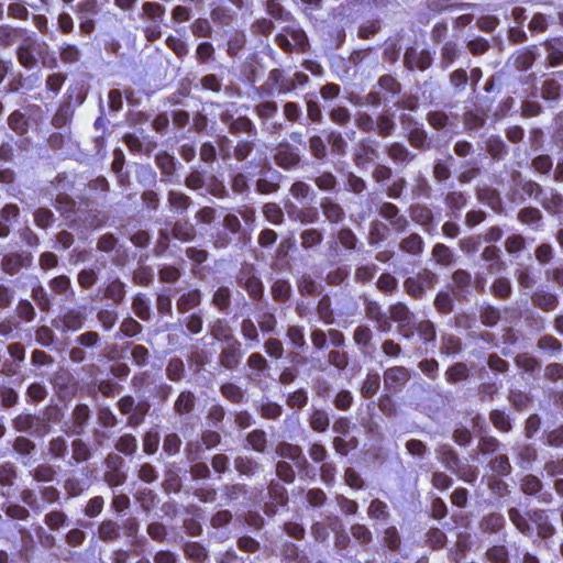
ically, in the local update, each client model will be opti-        model to optimize towards a converged optimal solution. As
mized towards its own local optima (i.e., fitting its individual    can be observed from the last two columns of Fig. 1, the pro-
feature distribution) instead of solving the global objective,      posed amplitude normalization for local harmonization well
which raises a drift across client updates. Meanwhile, in the       mitigates the distance between global and local solutions,
global update that aggregates these diverged local models,          and with the weight perturbation for global harmonization,
the server model is further distracted by the set of mismatch-      our approach achieves flat client solutions that can be di-
ing local optima, which subsequently leads to a global drift        rectly aggregated to obtain an optimal global model.
at the server model. Fig. 1 intuitively illustrates such local         Our main contributions are highlighted as follows:
and global drifts via loss landscape visualization (Li et al.        • We propose to effectively mitigate the local update drift
2018), in an example of two non-iid clients. The vertical axis         by normalizing the frequency-space amplitude compo-
shows the loss at each client (denoting the solution for global        nent of different images into a unified space, which har-
objective as F ∗ and for each local objective as Fi∗ ), and the        monizes non-iid features across clients.
horizontal plane represents a parameter space centered at the
                                                                     • Based on the harmonized features, we further design a
specific parameters of global model . With the same objec-
                                                                       novel weight-perturbation based strategy to rectify global
tive function and parameter initialization for each client, we
                                                                       server update shift without extra communication cost.
can see the local solution of two clients in the first column
are significantly different, which indicates the drift across lo-    • To the best of our knowledge, we are the first to simul-
cal client updates. Globally, a current good solution F ∗ may          taneously address both local and global update drifts for
achieve a relatively low loss for both clients. However, since         federated learning on heterogeneous medical images. We
each client has its own shaped loss landscape, optimizing              have also theoretically analyzed the proposed HarmoFL
the current solution towards global optima is difficult and            framework from the aspect of gradients similarity, show-
the aggregation of the two diverged local solutions further            ing that drift caused by data heterogeneity is bounded.
distracts the current good solution.                                 • We conduct extensive experiments on three medical im-
   To address such non-iid problem in FL, existing works               age tasks, including breast cancer histology image classi-
can be mainly divided into two groups, which correspond                fication, histology nuclei segmentation, and prostate MRI
to tackling the drift locally or globally. The local side em-          segmentation. Our HarmoFL significantly outperforms a
phasizes how to better normalize those diverse data. For ex-           set of latest state-of-the-art FL methods.
ample, (Sheller et al. 2018) conducted a pioneer study and
proposed using data pre-processing to reduce data hetero-                               2   Related Work
geneity. Recently, FedBN (Li et al. 2021) kept batch normal-        There have been many methods proposed trying to improve
ization layers locally to normalize local data distribution. As     federated learning on heterogeneous data and can be mainly
for the global server side, adjusting aggregation weight is a       divided into two groups, including improvements on local
typical strategy, for instance, (Yeganeh et al. 2020) used in-      client training and on global server aggregation.
verse distance to adaptively reweight aggregation. Recently,
the framework FedAdam (Reddi et al. 2021) is proposed for           Local client training: Literature towards improving the
introducing adaptive optimization to stabilize server update        client training to tackle local drift includes, using data
in heterogeneous data. However, these methods tackle het-           pre-processing to reduce data heterogeneity (Sheller et al.
erogeneity partially via either client or server update. The        2018), introducing a domain loss for heterogeneous elec-
local and global drifts are essentially coupled, yet how to         troencephalography classification (Gao et al. 2019), using
jointly solve them as a whole still remains unclear.                simulated CT volumes to mitigate scanner differences in
                                                                    cardiac segmentation (Li et al. 2020a), adding a proximal
   In this paper, we consider both client and server updates
                                                                    term to penalize client update towards smaller weight dif-
and propose a new harmonizing strategy to effectively solve
                                                                    ferences between client and server model (Li et al. 2020b),
the data heterogeneity problem for federated medical im-
                                                                    and learning affine transformation against shift under the as-
age analysis. First, to mitigate local drift at the local update,
                                                                    sumption that data follows an affine distribution (Reisizadeh
we propose a more effective normalization strategy via am-
                                                                    et al. 2020). Recently, both SiloBN (Andreux et al. 2020)
plitude normalization, which unifies amplitude components
                                                                    and FedBN (Li et al. 2021) propose keeping batch normal-
from images decomposed in the frequency domain. Then
                                                                    ization locally to help clients obtain similar feature distribu-
for the global drift, although weighted parameter aggrega-
                                                                    tions, and MOON (Li, He, and Song 2021) uses contrastive
tion is widely adopted, the coordination can fail over het-
                                                                    learning on latent feature representations at the client-side to
erogeneous clients with large parameter differences. Thus,
                                                                    enhance the agreements between local and global models.
we aim to promote client models that are easy to aggregate
rather than design a new re-weighting strategy. Based on the        Global server aggregation: Besides designs on the client-
harmonized feature space, we design a weight-perturbation           side, many methods are proposed towards reducing global
strategy to reduce the server update drift. The perturbation        drift with a focus on the server-side. (Zhao et al. 2018) create
is generated locally from gradients and applied on the client       a small subset of data that is globally shared across clients,
model to constrain a neighborhood area of the local con-            and many other methods improve the aggregation strategy,
verged model to have a uniformly low loss. With the pertur-         e.g. (Yeganeh et al. 2020) calculate the inverse distance
bation, each client finds a shared flat optimal solution that       to re-weight aggregation and FedNova (Wang et al. 2020)
can be directly aggregated with others, assisting the global        proposes to use normalized stochastic gradients to perform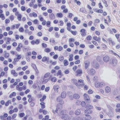
global model aggregation rather than the cumulative raw lo-
                                                                                                                     Shared
cal gradient changes. Very recently, FedAdam (Reddi et al.
2021) introduces adaptive optimization into federated learn-

                                                                                                         Normalize
ing to stabilize convergence in heterogeneous data.
   However, the above-mentioned methods partially address            Phase        Image      Amplitude

the drift either from the local client or global server perspec-
tive. Instead, our approach aims jointly mitigating the two
coupled drifts both locally and globally.

                     3   Methodology                               Figure 2: Amplitude normalization that harmonizes local
To address the non-iid issues from both local and global as-       client features. Phase components are strictly kept locally
pects, we propose an effective new federated learning frame-       and only the average amplitude from each client is shared.
work of HarmoFL. We start with the formulation of feder-
ated heterogeneous medical images analysis, then describe          transform images into the frequency space signals and de-
amplitude normalization and weight perturbation towards            compose out the amplitude spectrum which captures low-
reducing local drift and global drift respectively. At last, we    level features. Considering the patient level privacy sensitiv-
give a theoretical analysis of HarmoFL.                            ity and forbiddance of sharing original images, we propose
                                                                   only using averaged amplitude term during communication
3.1   Preliminaries                                                to conduct the normalization.
Denote (X , Y) as the joint image and label space over N              More specifically, for input image x from the i-th
clients. A data sample is an image-label pair (x, y) with x ∈      client, we transform each channel of image x ∈
X , y ∈ Y, and the data sampled from a specific i-th client        RH×W ×C into the frequency space signals F i (x)(u, v) =
follows data distribution Di . In this work, we focus on the       PH−1 PW −1               −j2π ( H
                                                                                                   h    w
                                                                                                     u+ W v)
non-iid feature shift. Given the joint probability P (x, y) of        h=0     w=0 x(h, w)e                   . Then we can split
feature x of image x and label y, we have Pi (x) varies even       the real part Ri (x) and the imaginary part Ii (x) from the
if P (y| x) is the same or Pi (x |y) varies across clients while   frequency signals F i (x). The amplitude and phase compo-
P (y) is unchanged.                                                nent can be expressed as:
                                                                                                               1/2
   Our proposed HarmoFL aims to improve federated learn-                           Ai (x) = R2i (x) + Ii2 (x)

ing for both local client training and global aggregation. The                                                                 (2)
federated optimization objective is formulated as follows:                        Pi (x) = arctan [Ii (x)/Ri (x)] .
                  "           N
                                                   #               Next, we normalize the amplitude component of each im-
                             X                                     age batch-wise with a moving average term. For the k-th
             min F (θ) :=        pi Fi (θ + δ, Di ) ,        (1)   batch of M sampled images, first we decompose the ampli-
             θ
                            i=1
                                                                   tude Ai,xm and phase P i,xm for each single image xm in
                                                                   the batch. We calculate the in-batch average amplitude and
                 P
where Fi =          (x,y)∼D i `i (Ψ(x), y; θ + δ) is the local
objective function and `i is the loss function defined by          update the average amplitude with a decay factor v:
the learned model θ and sampled pair (x, y). For the i-th                                                            1 X
                                                                                                                        M
client, pi is the corresponding weight such that pi ≥ 0 and                  Ai,k = (1 − v)Ai,k−1 + v                      Ai,xm ,   (3)
PN                                                                                                                   M m=1
   i=1 pi = 1. The δ is a weight perturbation term and D i is
the harmonized feature distribution obtained by our ampli-         where Ai,k−1 is the average amplitude calculated from the
tude normalization. Specifically, we propose a new ampli-          previous batch and this term is set to zero for the first batch.
tude normalization operator Ψ(·) harmonizing various client        The Ai,k harmonizes low-level distributions inside a client
features distribution to mitigate client update drift. The nor-    and keeps tracking amplitudes of the whole client images.
malizer manipulates amplitudes of data in the frequency            With the updated average term, each original image of the
space without violating the local original data preserving.        k-th batch is normalized using the average amplitude Ai,k
Based on the harmonized features, we can generate a weight         and its original phase component P i,xm in below:
perturbation for each client without any extra communica-
tion cost. The perturbation forces each client reaching a uni-                     Ψ(xm ) = F −1 (Ai,k , P i,xm ),                   (4)
formly low error in a neighborhood area of local optima,                     −1
                                                                   where F       is the inverse Fourier transform. After client
thus reducing the drift in the server.                             training, the amplitude normalization layer which only con-
                                                                   tains the average amplitude information will be sent to the
3.2   Amplitude normalization for local training                   central server and generate a global amplitude. This global
Structure semantic is an important factor to support med-          amplitude compromises various low-level visual features
ical imaging analysis while low-level statistics (e.g. color,      across clients and can help reduce client update drift at the
contrast) usually help to differentiate the structure. By de-      next federated round. In practice, we find that only commu-
composing the two parts, we are able to harmonize low-level        nication at the first round and fix the global amplitude can
features across hospitals while preserving critical structures.    well harmonize non-iid features as well as saving the com-
Using the fast Fourier transform (Nussbaumer 1981), we can         munication cost.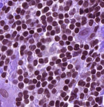
3.3   Weight perturbation for global aggregation                 Algorithm 1: Harmonizing Local and Global Drifts in FL
The above-proposed amplitude normalization allows each           Input: communication rounds T , number of clients N , mini-
client to optimize within a harmonized feature space, mit-       batch steps K, client learning rate ηl , global learning rate ηg ,
igating the local drift. Based on the harmonized feature         hyper-parameter α
space, we further aim to promote client models that are easy     Output: The final global model θ(T )
to aggregate, thus rectifying the global drift. As the global     1: Initialize server model θ (1)
aggregation is typically the weighted averaging, a client with    2: for t = 1, 2, · · · , T do
flat optima can well coordinate with other clients than sharp     3:     for i = 1, 2, · · · , N in parallel do
local minima (Keskar et al. 2016), which shows large er-          4:           t
                                                                              θi,1  ← θt . send the global model θt to client i
ror increases even with minor parameter change. Motivated         5:          for k = 1, 2, · · · , K do         . client training
from adversarial training, we propose a local optimization        6:               sample a batch of data pairs (x, y) of Di
objective of each client as below:                                                   t                t
                                                                  7:               Ai,k = (1 − v)Ai,k−1
                     X                                                                          1
                                                                                                   PM
              min             0
                                max `(x0 , y; θ),          (5)    8:                        +v M     m=1 Axm            . Eq. (3)
              θ               kx −xkp ≤δ                                                                         t
                  (x,y)∼D i                                       9:                Ψ(x) = F −1 (Ai,k , P xm )           . Eq. (4)
where x0 is the adversarial image within a Lp -norm bounded      10:
                                                                                             ∇`i (Ψ(x),y;θ)
                                                                                    δk = α k`i (Ψ(x),y;θ)k               . Eq. (6)
δ-ball centered at original image x, the adversarial image                                                 2
                                                                                                            t
                                                                 11:                gδ = ∇`i (Ψ(x), y; θi + δk )
is generated with the same label of x but different feature                          t          t
                                                                 12:                θi,k+1 ← θi,k   − ηl gδ              . Eq. (7)
shift. However, the generating process has an extra com-
munication burden since we have to transfer feature distri-      13:            end for
                                                                                         t
bution information across clients. Based on the harmonized       14:            return θi,K          . send client model to server
features, we carefully design a weight perturbation to effec-    15:        end for          PN
tively solve the Eq. (5). With a little abuse of notation, in-   16:        θt+1 ← θt − ηg i=1 pi (θi,K   t      t
                                                                                                              − θi,1 )
                                                                              t+1          N      t
stead of generating adversarial images bonded by the term δ,                          1
                                                                                        P
                                                                 17:        A     = N i=1 Ai,K
we propose a new δ as a perturbation that is directly applied    18:    end for
to model parameters. The perturbation is self-generated us-      19:    return θ(T )
ing gradients from the harmonized feature and has no extra
communication cost. Formally, for the k-th batch, we first
calculate the gradients of client model θi,k−1 on the am-        and weight perturbation from the gradients perspective. For
plitude normalized feature Ψ(x), which is calculated from        amplitude normalization, it reduces gradients dissimilarity
Eq. (4). Then we use the Euclidean norm k · k2 to normalize      between clients by harmonizing the non-iid features. In the
the gradients and obtain the perturbation term for the current   meanwhile, the weight perturbation forces clients to achieve
iteration of gradient descent:                                   flat optima, in which the loss variation is constrained, mak-
                        ∇`i (Ψ(x), y; θi,k−1 )                   ing the gradients change mildly. So both amplitude normal-
              δk = α                            ,         (6)    ization and weight perturbation bound gradient differences
                       k`i (Ψ(x), y; θi,k−1 )k2
                                                                 across clients, and this assumption has also been widely ex-
where α is a hyper-parameter to control the degree of per-       plored in different forms (Yin et al. 2018; Li et al. 2020b;
turbation. The flat area around the local client optimum can     Vaswani, Bach, and Schmidt 2019; Karimireddy et al. 2019).
be expanded with the larger α, and the choice of α is studied    Based on the standard federated optimization objective, we
in the experiment section. After obtaining the perturbation      formulate a new form in below:
term δk , we minimize the loss on the parameter-perturbated                        "          N
                                                                                                               #
model as below:
                                                                                              X
                                                                              min F (θ) :=       pi Fi (θ, Di )
                                                                                       θ
       θi,k ← θi,k−1 − ηl ∇`i (Ψ(x), y; θi,k−1 + δk ),    (7)                                              i=1
                                                                                  X                                                        (8)
where θi,k−1 is the model from the previous batch and ηl is            s.t.                     |∇`(xi , yi ; θ) − ∇`(xj , yj ; θ)| ≤ ,
the local client learning rate. After iteratively update, each                (xi ,yi )∼D i ,
                                                                              (xj ,yj )∼D j
local client model is gradually driven towards an optimal
solution that holds a uniformly low loss around its neighbor-    where j ∈ {1, · · · , N }\{i} and  is a non-negative constant
hood area (i.e. flat optimum), thus promoting the aggrega-       and (xi , yi ) is the image-label pair from the i-th client’s dis-
tion and getting rid of trapped into the local sharp minima.     tribution. To quantify the overall drift between client and
                                                                 server models at the t-th communication round, we define
3.4   Theoretical analysis for HarmoFL                           the overall drift term as below:
With the help of amplitude normalization and weight per-                                           K N
turbation, we constrain the client update with less dissim-                                      1 XX        t
                                                                                     Γ=                  E[kθi,k − θt k2 ],                (9)
ilarity and achieve a model having a relatively low error                                       KN   i=1
                                                                                                     k=1
with a range of parameter changes. To theoretically ana-
lyze HarmoFL, we transform our approach into a simplified        where K is the mini-batch steps. We theoretically show that
setting where we interpret both the amplitude normalization      with the bounded gradient difference, our HarmoFL strategy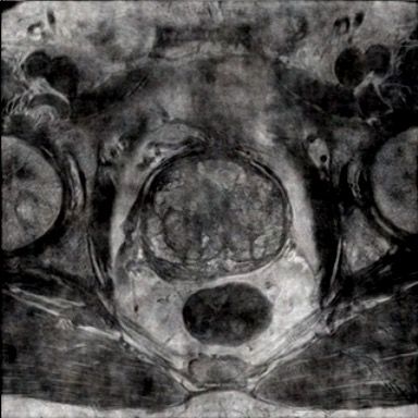
is guaranteed to have an upper bound on the overall drift         with 1 local update epoch for each communication round.
caused by non-iid data.                                           We use segmentation Dice coefficient (Dice) loss and SGD
Theorem 3.1 With the shift term Γ defined in Eq. (9), as-         optimizer with a learning rate of 1e−4 .
sume the gradient dissimilarity and variance are bounded          Prostate MRI segmentation. For the prostate segmenta-
and the functions Fi are β-smooth, denote the effective step-     tion, we use a multi-site prostate segmentation dataset (Liu
size η̃ = Kηg ηl , we have the upper bound for the overall        et al. 2020) which contains 6 different data sources from 3
drift of our HarmoFL below:                                       public datasets (Nicholas et al. 2015; Lemaı̂tre et al. 2015;
             N                                                    Litjens et al. 2014). We regard each data source as a client
          1 X 4η̃ 2          2   4η̃ 2 2 (N − 1)2   2η̃ 2 σ 2    and train the U-Net using Adam optimizer with a learning
 Γ≤                 k∇Fi (θ)k  +                   +
          N i=1 ηg2                     ηg2 N 2       Kηg2        rate of 1e−4 , momentum of 0.9 and 0.99.
                                                                     We report the performance of global models, i.e., the final
          4η̃ 2 (G2 + B 2 C 2 ) 4η̃ 2 2 (N − 1)2   2η̃ 2 σ 2     results of our overall framework. The model was selected
      ≤                        +                  +           ,
                   ηg2                 ηg2 N 2       Kηg2         using the separate validation set and evaluated on the testing
                                                                  set. To avoid distracting focus on the feature non-iid problem
where C := F (θ0 ) − F ∗ when functions Fi are convex,            due to data imbalance, we truncate the sample size of each
and for non-convex situation, we have C := k∇F (θ)k. This         client to their respective smaller number in histology image
theorem gives the upper bound with both the convex and            classification and prostate MRI segmentation task, but we
non-convex assumptions for Fi .                                   keep the client data imbalance in the nuclei segmentation
   Please find the notation table in Appendix A. All assump-      task to demonstrate the performance with data quantity dif-
tions and proofs are formally given in Appendix B. The            ference. If not specified, our default setting for the local up-
proof sketch is applying our extra gradient differences con-      date epoch is 1. We use the momentum of 0.9 and weight
straint in the subproblem of one round optimization and us-       decay of 1e−4 for all optimizers in three tasks. We empiri-
ing the bounded dissimilarity. The shift bound is finally un-     cally set the decay factor v to 0.1 and set the degree of per-
rolled from a recursion format of one round progress.             turbation term to 5e−2 by grid search. For more dataset and
                                                                  implementation details, please refer to Appendix C.
                        4    Experiments
In this section, we extensively evaluate our method to                     Client A   Client B   Client C   Client D    Client E
demonstrate that harmonizing local and global drifts are
                                                                  Normal

beneficial for clients with heterogeneous features. Our har-
monizing strategy, HarmoFL, achieves higher performance
as well as more stable convergence compared with other
methods on feature non-iid datasets. This is shown on the
breast cancer histology image classification, histology nu-
                                                                  Tumor

clei segmentation, and prostate MRI segmentation. All re-
sults reported are the average of three repeating runs with a
standard deviation of different random seeds. More results        Figure 3: Examples of breast histology images of normal and
please refer to Appendix C.                                       tumor tissues from five clients, showing large heterogeneity.
4.1       Dataset and experimental settings
Breast cancer histology image classification. We use the          4.2        Comparison with the state-of-the-arts
public tumor dataset Camelyon17, which contains 450,000
                                                                  We compare our approach with recent state-of-the-art
histology images with different stains from 5 different hos-
                                                                  (SOTA) FL methods towards solving the non-iid problem.
pitals (Bandi et al. 2018). As shown in Fig. 3, we take each
                                                                  For local drifts, FedBN (Li et al. 2021) focuses on the non-
hospital as a single client, and images from different clients
                                                                  iid feature shift with medical image applications, and both
have heterogeneous appearances but share the same label
                                                                  FedProx (Li et al. 2020b) and a recent method MOON (Li,
distribution (i.e. normal and tumor tissues). We use a deep
                                                                  He, and Song 2021) tackle the non-iid problem by con-
network of DenseNet121 (Huang et al. 2017) and train the
                                                                  straining the dissimilarity between local and global mod-
model for 100 epochs at the client-side with different com-
                                                                  els to reduce global aggregation shifts. FedAdam (Reddi
munication frequencies. We use cross-entropy loss and SGD
                                                                  et al. 2021) and FedNova (Wang et al. 2020) are proposed
optimizer with a learning rate of 1e−3 .
                                                                  as general methods to tackle global drifts. For the breast
Histology nuclei segmentation. For the cell nuclei seg-           cancer histology image classification shown in Table 2, we
mentation, we gather three public datasets, including             report the testing accuracy on five different clients and the
MoNuSAC2020 (Verma et al. 2021), MoNuSAC2018 (Ku-                 average results. FedProx only achieves minor improvements
mar et al. 2019) and TNBC (Naylor et al. 2018). For data          than FedAvg, showing that only reducing global aggregation
from MoNuSAC2020, we divide them into 4 clients accord-           drift may not achieve promising results when local clients
ing to different hospitals they come from and form 6 clients      shifted severely. Another recent representation dissimilarity
in total. We use U-Net (Ronneberger, Fischer, and Brox            constraining method, MOON, boosts the accuracy on clients
2015) and train the model for 500 communication rounds            B, C, D but suffers from a large drop on client E. The reason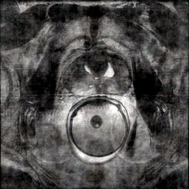
Table 1: Results for histology nuclei segmentation and prostate MRI segmentation. The results of the Dice coefficient are
reported. Each column represents one client and the Avg. is abbreviated for the average Dice.
                        Histology Nuclei Segmentation (Dice %)      Prostate MRI Segmentation (Dice %)
       Method
                      A     B      C      D     E       F    Avg. A    B      C     D      E      F    Avg.
         FedAvg     73.44 73.06 72.52 68.91 67.33 49.69 67.49 90.04 94.31 92.60 92.21 90.14 89.36 91.44
    (PMLR2017)      (0.02) (0.24) (0.85) (0.34) (0.86) (0.34) (9.06)   (1.27) (0.28) (0.66) (0.71) (0.27) (1.76) (1.91)
        FedProx     73.49 73.11 72.45 69.01 67.33 49.56 67.49 90.65 94.60 92.64 92.19 89.36 87.07 91.08
    (MLSys2020)     (0.07) (0.19) (0.94) (0.34) (0.86) (0.34) (9.12)   (1.95) (0.30) (1.03) (0.15) (0.97) (1.53) (2.66)
        FedNova     73.40 73.01 71.50 69.23 67.46 50.68 67.55 90.73 94.26 92.73 91.91 90.01 89.94 91.60
   (NeurIPS2020)    (0.05) (0.38) (1.35) (0.34) (1.07) (0.34) (8.57)   (0.41) (0.08) (1.29) (0.61) (0.87) (1.54) (1.70)
        FedAdam     73.53 72.91 71.74 69.26 66.69 49.72 67.31 90.02 94.84 93.30 91.70 90.17 87.77 91.30
      (ICLR2021)    (0.08) (0.24) (1.33) (0.50) (1.18) (0.11) (8.98)   (0.29) (0.11) (0.79) (0.16) (1.46) (1.35) (2.53)
         FedBN      72.50 72.51 74.25 64.84 68.39 69.11 70.27 92.68 94.83 93.77 92.32 93.20 89.68 92.75
      (ICLR2021)    (0.81) (0.13) (0.28) (0.93) (1.13) (0.94) (3.47)   (0.52) (0.47) (0.41) (0.19) (0.45) (0.60) (1.74)
         MOON       72.85 71.92 69.23 69.00 65.08 48.26 66.06 91.79 93.63 93.01 92.61 91.22 91.14 92.23
     (CVPR2021)     (0.46) (0.37) (2.29) (0.71) (0.73) (0.66) (9.13)   (1.64) (0.21) (0.75) (0.53) (0.61) (0.88) (1.01)
        HarmoFL     74.98 75.21 76.63 76.59 73.94 69.20 74.42 94.06 95.26 95.28 93.51 94.05 93.53 94.28
         (Ours)     (0.36) (0.57) (0.20) (0.77) (0.13) (1.23) (2.76)   (0.47) (0.38) (0.33) (0.79) (0.50) (1.02) (0.80)

Table 2: Results for breast cancer histology images classi-     images show fewer non-iid feature shifts than histology im-
fication of different methods. Each column represents one       ages, the performance gap of each client is not as large as
client and the Avg. is abbreviated for the average accuracy.    nuclei segmentation. However, our method still consistently
               Breast Cancer Histology Image Classification     achieves the highest Dice of 94.28% and has a smaller stan-
    Method                    (Accuracy %)                      dard deviation over different clients. Besides, we visualize
                A      B       C       D      E       Avg.      the segmentation results to demonstrate a qualitative com-
      FedAvg  91.10 83.12 82.06 87.49 74.78 83.71               parison, as shown in Fig. 4. Comparing with the first ground-
 (PMLR2017) (0.46) (1.58) (8.52) (2.49) (3.19) (6.16)           truth column, due to the heterogeneous features, other fed-
     FedProx  91.03 82.88 82.78 87.07 74.93 83.74               erated learning methods either cover more or fewer areas
 (MLSys2020) (0.50) (1.63) (8.56) (1.76) (3.05) (5.99)          in both prostate MRI and histology images. As can be ob-
     FedNova  90.99 82.97 82.40 86.93 74.86 83.61               served from the second and fourth row, the heterogeneity in
(NeurIPS2020) (0.54) (1.76) (9.21) (1.58) (3.12) (6.00)
                                                                features also makes other methods fail to obtain an accurate
     FedAdam  87.45 80.38 76.89 89.27 77.86 82.37               boundary. But with the proposed harmonizing strategy, our
   (ICLR2021) (0.77) (2.03) (14.03) (1.28) (2.68) (5.65)
      FedBN   89.35 90.25 94.16 94.04 68.87 87.33
                                                                approach shows more accurate and smooth boundaries.
   (ICLR2021) (8.50) (1.66) (1.00) (2.32) (22.14) (10.55)
      MOON    88.92 83.52 84.71 90.02 67.79 82.99               4.3    Ablation study
  (CVPR2021) (1.54) (0.31) (5.14) (1.56) (2.06) (8.93)
     HarmoFL   96.17 93.60 95.54 95.58 96.50 95.48              We further conduct ablation study based on the breast
      (Ours)  (0.56) (0.67) (0.32) (0.27) (0.46) (1.13)         cancer histology image classification to investigate key
                                                                properties of our HarmoFL, including the convergence
                                                                analysis, influence of different local update epochs, and the
                                                                effects of weight perturbation degree.
may come from that images in client E appear differently
as shown in Fig. 3, making the representations of client E      Convergence analysis. To demonstrate the effective-
failed to be constrained towards other clients. With the har-   ness of our method on reducing local update and server
monized strategy reducing both local and global drifts, our     update drifts, we plot the testing accuracy curve on the
method consistently outperforms others, reaching an accu-       average of five clients for 100 communication rounds with
racy of 95.48% on average, which is 8% higher than the pre-     1 local update epoch. As shown in Fig. 5(a), the curve of
vious SOTA (FedBN) for the feature non-iid problem. Be-         HarmoFL increases smoothly with communication rounds
sides, our method can help all heterogeneous clients bene-      increasing, while the state-of-the-art method of FedBN (Li
fit from the federated learning, where clients show a testing   et al. 2021), shows unstable convergence as well as lower
accuracy with a small standard deviation on average, while      accuracy. From the curve of FedBN (Li et al. 2021), we
other methods show larger variance across clients.              can see the there are almost no improvements at the first 10
    For segmentation tasks, the experimental results of Dice    communication rounds, the potential reason is that the batch
are shown in Table 1 in the form of single client and average   normalization layers in each local client model are not fully
performance. On histology nuclei segmentation, HarmoFL          trained to normalize feature distributions.
significantly outperforms the SOTA method of FedBN and
improves at least 4% on mean accuracy compared with all         Influence of local update epochs. Aggregating with
other methods. On the prostate segmentation task, as MRI        different frequencies may affect the learning behavior,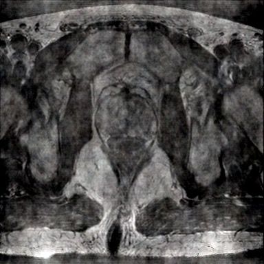
Groundtruth         FedAvg     FedProx         FedNova    FedAdam        FedBN         MOON       HarmoFL (Ours)

Figure 4: Qualitative comparison on segmentation results with our method and other state-of-the-art methods. Top two rows for
the task of prostate MRI segmentation and the bottom two rows for the task of histology nuclei segmentation.

                                                                 significantly outperforms other approaches and shows ro-
                                                                 bustness to larger drift brought by more local update epochs.

                                                                 Effects of weight perturbation degree. We further
                                                                 analyze how the weight perturbation degree control
                                                                 hyper-parameter α affects the performance of our method.
                               (a)                               Intuitively, the value of α indicates the radius of the flat
                                                                 optima area. A small radius may hinder clients to find a
                                                                 shared flat area during aggregation, while a large radius
                                                                 creates difficulties in the optimization of reaching such a flat
                                                                 optimum. As shown in Fig 5(c), we plot the average testing
                                                                 accuracy with standard error across clients by searching
                                                                 α ∈ {1, 5e−1 , 5e−2 , 5e−3 , 5e−4 }. Our method reaches the
                                                                 highest accuracy when α = 5e−2 and the performance
                    (b)                        (c)
                                                                 decreases with α reducing. Besides, we can see our method
Figure 5: (a) Convergence in terms of testing accuracy with      can achieve more than 90% accuracy even without degree
communication rounds. (b) Comparison of FedAvg, FedBN,           control (i.e. α = 1).
and our HarmoFL with different local training epochs. (c)
Performance of HarmoFL with different perturbation radius.                             5   Conclusion
                                                                 This work proposes a novel harmonizing strategy, HarmoFL,
since less frequent communication will further enhance           which uses amplitude normalization and weight perturba-
the drift due to the non-iid feature, and finally obtaining      tion to tackle the drifts that exist in both local client and
a worse global model. We study the effectiveness of Har-         global server. Our solution gives inspiration on simultane-
moFL with different local update epochs and the results          ously solving the essentially coupled local and global drifts
are shown in Fig. 5(b). When the local epoch is 1, each          in FL, instead of regarding each drift as a separate issue.
client communicates with others frequently, all methods          We conduct extensive experiments on heterogeneous med-
have a relatively high testing accuracy. With more local         ical images, including one classification task and two seg-
epochs added, the local client update drift is increased and     mentation tasks, and demonstrates the effectiveness of our
the differences between local and global models become           approach consistently. We further provide theoretical anal-
larger. Both FedAvg and FedBN suffer from large drifts           ysis to support the empirical results by showing the overall
and show severe performance drops. However, because              non-iid drift caused by data heterogeneity is bounded in our
our method enables each client to train the model using          proposed HarmoFL. Overall, our work is beneficial to pro-
weight perturbation with harmonized features, HarmoFL            mote wider impact of FL in real world medical applications.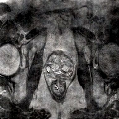
References                                 Karimireddy, S. P.; Kale, S.; Mohri, M.; Reddi, S.; Stich, S.;
Andreux, M.; du Terrail, J. O.; Beguier, C.; and Tramel,           and Suresh, A. T. 2020. SCAFFOLD: Stochastic Controlled
E. W. 2020. Siloed federated learning for multi-centric            Averaging for Federated Learning. In III, H. D.; and Singh,
histopathology datasets. In Domain Adaptation and Rep-             A., eds., Proceedings of the 37th International Conference
resentation Transfer, and Distributed and Collaborative            on Machine Learning, volume 119 of Proceedings of Ma-
Learning, 129–139. Springer.                                       chine Learning Research, 5132–5143. PMLR.
                                                                   Karimireddy, S. P.; Kale, S.; Mohri, M.; Reddi, S. J.; Stich,
Aubreville, M.; Bertram, C. A.; Donovan, T. A.; Marzahl,
                                                                   S. U.; and Suresh, A. T. 2019. SCAFFOLD: Stochastic Con-
C.; Maier, A.; and Klopfleisch, R. 2020. A completely an-
                                                                   trolled Averaging for On-Device Federated Learning.
notated whole slide image dataset of canine breast cancer
to aid human breast cancer research. Scientific data, 7(1):        Keskar, N. S.; Mudigere, D.; Nocedal, J.; Smelyanskiy,
1–10.                                                              M.; and Tang, P. T. P. 2016. On large-batch training for
                                                                   deep learning: Generalization gap and sharp minima. arXiv
Bandi, P.; Geessink, O.; Manson, Q.; Van Dijk, M.; Balken-         preprint arXiv:1609.04836.
hol, M.; Hermsen, M.; Bejnordi, B. E.; Lee, B.; Paeng, K.;
Zhong, A.; et al. 2018. From detection of individual metas-        Kumar, N.; Verma, R.; Anand, D.; Zhou, Y.; Onder, O. F.;
tases to classification of lymph node status at the patient        Tsougenis, E.; Chen, H.; Heng, P.-A.; Li, J.; Hu, Z.; et al.
level: the CAMELYON17 challenge. IEEE Transactions on              2019. A multi-organ nucleus segmentation challenge. IEEE
Medical Imaging.                                                   transactions on medical imaging, 39(5): 1380–1391.
Dhruva, S. S.; Ross, J. S.; Akar, J. G.; Caldwell, B.; Childers,   Lemaı̂tre, G.; Martı́, R.; Freixenet, J.; Vilanova, J. C.;
K.; Chow, W.; Ciaccio, L.; Coplan, P.; Dong, J.; Dykhoff,          Walker, P. M.; and Meriaudeau, F. 2015. Computer-aided
H. J.; et al. 2020. Aggregating multiple real-world data           detection and diagnosis for prostate cancer based on mono
sources using a patient-centered health-data-sharing plat-         and multi-parametric MRI: a review. Computers in biology
form. NPJ digital medicine, 3(1): 1–9.                             and medicine, 60: 8–31.
                                                                   Li, D.; Kar, A.; Ravikumar, N.; Frangi, A. F.; and Fidler, S.
Dou, Q.; So, T. Y.; Jiang, M.; Liu, Q.; Vardhanabhuti, V.;         2020a. Federated Simulation for Medical Imaging. In Med-
Kaissis, G.; Li, Z.; Si, W.; Lee, H. H.; Yu, K.; et al. 2021.      ical Image Computing and Computer Assisted Intervention
Federated deep learning for detecting COVID-19 lung ab-            (MICCAI), 159–168.
normalities in CT: a privacy-preserving multinational vali-
dation study. NPJ digital medicine, 4(1): 1–11.                    Li, H.; Xu, Z.; Taylor, G.; Studer, C.; and Goldstein, T. 2018.
                                                                   Visualizing the Loss Landscape of Neural Nets. In Neural
Gao, D.; Ju, C.; Wei, X.; Liu, Y.; Chen, T.; and Yang, Q.          Information Processing Systems.
2019. Hhhfl: Hierarchical heterogeneous horizontal feder-
ated learning for electroencephalography. arXiv preprint           Li, Q.; He, B.; and Song, D. 2021. Model-Contrastive Feder-
arXiv:1909.05784.                                                  ated Learning. In Proceedings of the IEEE/CVF Conference
                                                                   on Computer Vision and Pattern Recognition, 10713–10722.
Geiping, J.; Bauermeister, H.; Dröge, H.; and Moeller, M.
                                                                   Li, T.; Sahu, A. K.; Zaheer, M.; Sanjabi, M.; Talwalkar, A.;
2020. Inverting Gradients–How easy is it to break privacy
                                                                   and Smith, V. 2020b. Federated optimization in heteroge-
in federated learning? arXiv preprint arXiv:2003.14053.
                                                                   neous networks. In Conference on Machine Learning and
Hsieh, K.; Phanishayee, A.; Mutlu, O.; and Gibbons, P.             Systems.
2020. The non-iid data quagmire of decentralized machine           Li, X.; Huang, K.; Yang, W.; Wang, S.; and Zhang, Z. 2019.
learning. In International Conference on Machine Learning,         On the Convergence of FedAvg on Non-IID Data. In Inter-
4387–4398. PMLR.                                                   national Conference on Learning Representations.
Huang, G.; Liu, Z.; Van Der Maaten, L.; and Weinberger,            Li, X.; Jiang, M.; Zhang, X.; Kamp, M.; and Dou, Q. 2021.
K. Q. 2017. Densely connected convolutional networks. In           FedBN: Federated Learning on Non-IID Features via Lo-
Proceedings of the IEEE conference on computer vision and          cal Batch Normalization. In International Conference on
pattern recognition, 4700–4708.                                    Learning Representations.
Ju, C.; Gao, D.; Mane, R.; Tan, B.; Liu, Y.; and Guan, C.          Litjens, G.; Toth, R.; van de Ven, W.; Hoeks, C.; Kerkstra,
2020. Federated transfer learning for eeg signal classifica-       S.; van Ginneken, B.; Vincent, G.; Guillard, G.; Birbeck, N.;
tion. In 2020 42nd Annual International Conference of the          Zhang, J.; et al. 2014. Evaluation of prostate segmentation
IEEE Engineering in Medicine & Biology Society (EMBC),             algorithms for MRI: the PROMISE12 challenge. Medical
3040–3045. IEEE.                                                   image analysis, 18(2): 359–373.
Kairouz, P.; McMahan, H. B.; Avent, B.; Bellet, A.; Bennis,        Liu, Q.; Dou, Q.; Yu, L.; and Heng, P. A. 2020. Ms-net:
M.; Bhagoji, A. N.; Bonawitz, K.; Charles, Z.; Cormode, G.;        Multi-site network for improving prostate segmentation with
Cummings, R.; et al. 2019. Advances and open problems in           heterogeneous mri data. IEEE Transactions on Medical
federated learning. arXiv preprint arXiv:1912.04977.               Imaging.
Kaissis, G. A.; Makowski, M. R.; Rückert, D.; and Braren,         McMahan, B.; Moore, E.; Ramage, D.; Hampson, S.; and
R. F. 2020. Secure, privacy-preserving and federated ma-           y Arcas, B. A. 2017. Communication-efficient learning of
chine learning in medical imaging. Nature Machine Intelli-         deep networks from decentralized data. In Artificial Intelli-
gence, 2(6): 305–311.                                              gence and Statistics, 1273–1282.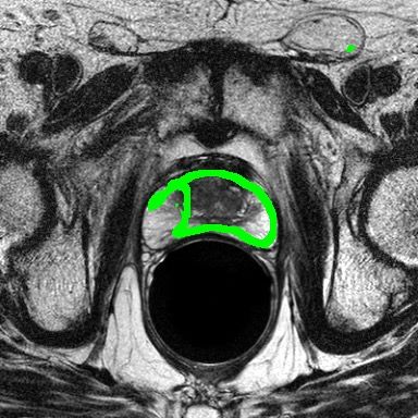
Naylor, P.; Laé, M.; Reyal, F.; and Walter, T. 2018. Segmen-      accelerated perceptron. In The 22nd International Con-
tation of nuclei in histopathology images by deep regression       ference on Artificial Intelligence and Statistics, 1195–1204.
of the distance map. IEEE transactions on medical imaging,         PMLR.
38(2): 448–459.                                                    Verma, R.; Kumar, N.; Patil, A.; Kurian, N. C.; Rane, S.;
Nicholas, B.; Anant, M.; Henkjan, H.; John, F.; Justin, K.;        Graham, S.; Vu, Q. D.; Zwager, M.; Raza, S. E. A.; Rajpoot,
et al. 2015. Nci-proc. ieee-isbi conf. 2013 challenge: Au-         N.; et al. 2021. MoNuSAC2020: A Multi-organ Nuclei Seg-
tomated segmentation of prostate structures. The Cancer            mentation and Classification Challenge. IEEE Transactions
Imaging Archive.                                                   on Medical Imaging.
Nussbaumer, H. J. 1981. The fast Fourier transform. In             Wang, J.; Liu, Q.; Liang, H.; Joshi, G.; and Poor, H. V. 2020.
Fast Fourier Transform and Convolution Algorithms, 80–             Tackling the Objective Inconsistency Problem in Heteroge-
111. Springer.                                                     neous Federated Optimization. Advances in Neural Infor-
                                                                   mation Processing Systems, 33.
Peiffer-Smadja, N.; Maatoug, R.; Lescure, F.-X.;
D’ortenzio, E.; Pineau, J.; and King, J.-R. 2020. Ma-              Xu, J.; Glicksberg, B. S.; Su, C.; Walker, P.; Bian, J.; and
chine learning for COVID-19 needs global collaboration             Wang, F. 2021. Federated learning for healthcare informat-
and data-sharing.       Nature Machine Intelligence, 2(6):         ics. Journal of Healthcare Informatics Research, 5(1): 1–19.
293–294.                                                           Yeganeh, Y.; Farshad, A.; Navab, N.; and Albarqouni, S.
Reddi, S. J.; Charles, Z.; Zaheer, M.; Garrett, Z.; Rush, K.;      2020. Inverse distance aggregation for federated learning
Konečný, J.; Kumar, S.; and McMahan, H. B. 2021. Adap-           with non-iid data. In Domain Adaptation and Representa-
tive Federated Optimization. In International Conference on        tion Transfer, and Distributed and Collaborative Learning,
Learning Representations.                                          150–159. Springer.
                                                                   Yin, D.; Pananjady, A.; Lam, M.; Papailiopoulos, D.; Ram-
Reisizadeh, A.; Farnia, F.; Pedarsani, R.; and Jadbabaie, A.
                                                                   chandran, K.; and Bartlett, P. 2018. Gradient diversity: a key
2020. Robust federated learning: The case of affine distribu-
                                                                   ingredient for scalable distributed learning. In International
tion shifts. arXiv preprint arXiv:2006.08907.
                                                                   Conference on Artificial Intelligence and Statistics, 1998–
Rieke, N.; Hancox, J.; Li, W.; Milletari, F.; Roth, H. R.; Al-     2007. PMLR.
barqouni, S.; Bakas, S.; Galtier, M. N.; Landman, B. A.;           Zhao, Y.; Li, M.; Lai, L.; Suda, N.; Civin, D.; and Chan-
Maier-Hein, K.; et al. 2020. The future of digital health with     dra, V. 2018. Federated learning with non-iid data. arXiv
federated learning. NPJ digital medicine, 3(1): 1–7.               preprint arXiv:1806.00582.
Ronneberger, O.; Fischer, P.; and Brox, T. 2015. U-net: Con-
volutional networks for biomedical image segmentation. In
International Conference on Medical image computing and
computer-assisted intervention, 234–241. Springer.
Roth, H. R.; Chang, K.; Singh, P.; Neumark, N.; Li, W.;
Gupta, V.; Gupta, S.; Qu, L.; Ihsani, A.; Bizzo, B. C.; et al.
2020. Federated learning for breast density classification:
A real-world implementation. In Domain Adaptation and
Representation Transfer, and Distributed and Collaborative
Learning, 181–191. Springer.
Sheller, M. J.; Edwards, B.; Reina, G. A.; Martin, J.; Pati, S.;
Kotrotsou, A.; Milchenko, M.; Xu, W.; Marcus, D.; Colen,
R. R.; et al. 2020. Federated learning in medicine: facilitat-
ing multi-institutional collaborations without sharing patient
data. Scientific reports, 10(1): 1–12.
Sheller, M. J.; Reina, G. A.; Edwards, B.; Martin, J.; and
Bakas, S. 2018. Multi-institutional deep learning model-
ing without sharing patient data: A feasibility study on brain
tumor segmentation. In International MICCAI Brainlesion
Workshop, 92–104. Springer.
Shilo, S.; Rossman, H.; and Segal, E. 2020. Axes of a rev-
olution: challenges and promises of big data in healthcare.
Nature medicine, 26(1): 29–38.
Tong, Q.; Liang, G.; and Bi, J. 2020. Effective federated
adaptive gradient methods with non-iid decentralized data.
arXiv preprint arXiv:2009.06557.
Vaswani, S.; Bach, F.; and Schmidt, M. 2019. Fast and faster
convergence of sgd for over-parameterized models and an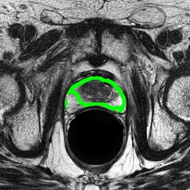
Roadmap of Appendix: The Appendix is organized as B.1 Assumptions
follows. We list the notations table in Section A. We pro- Assumption B.1 (β-smooth) {Fi } are β-smooth and satisfy
vide formal assumptions, theoretical analysis, and proof of
k∇Fi (θ) − ∇Fi (θi )k ≤ βkθ − θi k, for any i, θ, θi
bounded non-iid drift in Section B. The details of the exper-
imental setting and additional results are in Section C. Assumption B.2 (bounded gradient dissimilarity)
there exist constants G ≥ 0 and B ≥ 1 such that
N
A Notation Table 1 X 2
k∇Fi (θ)k ≤ G2 + B 2 k∇F (θ)k2 , ∀θ
N i=1
Notations Description if {Fi } are convex, we can relax the assumption to
F global objective function. N
1 X 2
Fi local objective function. k∇Fi (θ)k ≤ G2 + 2βB 2 (F (θ) − F ∗ ), ∀θ
N i=1
(X , Y) joint image and label space.
(x, y) a pair of data sample. Assumption B.3 (bounded variance) gi (θ) := ∇Fi (θ; xi )
T communication rounds. is unbiased stochastic gradient of Fi with bounded variance
N number of clients. 2
K mini-batch steps. E [kgi (θ) − ∇Fi (θ)k ] ≤ σ 2 , for any i, θ
xi
M size of sampled images in one batch. Lemma B.4 (relaxed triangle inequality) Let a1 , · · · , an be
`i
loss function defined by the learned model n vectors in Rd . Then the following are true:
and sampled pair.
2 2 1 2
weight in the federated optimization 1. kai + aj k ≤ (1 + γ) kai k + 1 + kaj k
pi γ
objective of the i-th client.
Di data distribution for the i-th client. , for any γ > 0
Ψ(·) the amplitude normalization operation.
n n
distribution harmonized by X X 2
Di amplitude normalization. 2.k ai k2 ≤ n kai k .
i=1 i=1
Ai,xm amplitude for each single image in a batch.
P i,xm phase for each single image in a batch. Proof: The proof of the first statement for any γ > 0 follows
from the identity:
average amplitude calculated from
Ai,k the current batch. kai + aj k =
2
δ perturbation applied to model parameters.
1
√ 1
2
2 2
hyper-parameter to control the degree (1 + γ) kai k + 1 + kaj k − γai + √ aj .
α γ γ
of perturbation.
ηl client model learning rate. For the second inequality, we use the convexity of x → kxk2
ηg global model learning rate. and Jensen’s inequality
2
η̃ effective step-size. 1X
n
1X
n
2
global server model at the t-th ai ≤ kai k .
θt n i=1 n i=1
communication round.
t
θi,k the i-th client model after k mini-batch steps.
Lemma B.5 (separating mean and variance) Let
gδ gradients of weight with perturbation.
{Ξ1 , . . . , Ξτ } be n random variables in Rd which are
a non-negative constant to bound gradients not necessarily independent. First suppose that their mean
difference. is E [Ξi ] = ξi and variance is bounded as E [Ξi − ξi ] ≤ σ 2 .
Γ overall non-iid drift term. Then, the following holds
Xn n
X
Table 3: Notations occurred in the paper. E[k 2
Ξi k ] ≤ k ξi k2 + n2 σ 2 .
i=1 i=1
Proof. For any random variable X, E[X 2 ] = (E[X −
B Theoretical analysis of bounded drift E[X]])2 + (E[X])2 implying
Xn n
X n
X
We give the theoretical analysis and proofs of HarmoFL in E[k Ξi k2 ] = k ξi k2 + E[k Ξi − ξi k2 ],
this section. First, we state the convexity, smoothness, and i=1 i=1 i=1
bounder gradient assumptions about the local function Fi expand the above equation using Lemma B.4, we can have
and global function F , which are typically used in optimiza- n n
tion literature (Li et al. 2020b; Reddi et al. 2021; Karim-
X X
E[k Ξi − ξi k2 ] ≤ τ E[kΞi − ξi k2 ] ≤ n2 σ 2 .
ireddy et al. 2020; Tong, Liang, and Bi 2020). i=1 i=1B.2 Theorem of bounded drift and proof follow the assumptions on gradients. Up to now, we get the
We first restate the Theorem 3.1 with some additional recursion format and then we unroll this and get below:
details and then give the proof. Recall that Γ = k−1
PK PN X 1 2η̃ 2
1
k=1
t t 2
i=1 E[kθi,k − θ k ].
E kθi,k − θk2 ≤ (1 + )ω ( 2 k∇Fi (θ)k2
KN
ω=1
K −1 ηg K
Theorem B.6 Suppose that the functions {Fi } satisfies as-
sumptions B.1, B.2 and B.3. Denote the effective step-size η̃ 2 σ 2 2η̃ 2 2 (N − 1)2
+ + )
η̃ = Kηg ηl , then the updates of HarmoFL have a bounded K 2 ηg2 ηg2 KN 2
drift: 2η̃ 2 2η̃ 2 2 (N − 1)2
≤ 2K( 2
k∇Fi (θ)k2 + )
• Convex: ηg K ηg2 KN 2
4η̃ 2 G2 4η̃ 2 2 (N − 1)2 2η̃ 2 σ 2 η̃ 2 σ 2
Γ≤ + + + ,
ηg 2 2
ηg N 2 Kηg2 K 2 ηg2
8β η̃ 2 B 2 averaging over i and k, if {Fi } are non-convex, we can have
+ (F (θ) − F ∗ ).
ηg2 N
1 X 4η̃ 2 2 4η̃ 2 2 (N − 1)2 2η̃ 2 σ 2
Γ≤ k∇Fi (θ)k + +
• Non-convex: N i=1 ηg2 ηg2 N 2 Kηg2
4η̃ 2 (G2 + B 2 k∇F (θ)k2 ) 4η̃ 2 2 (N − 1)2 4η̃ 2 G2 4η̃ 2 2 (N − 1)2 2η̃ 2 σ 2
Γ≤ + ≤ + +
ηg2 ηg2 N 2 ηg2 ηg2 N 2 Kηg2
2η̃ 2 σ 2 4η̃ 2 B 2
+ . + k∇F (θ)k2 .
Kηg2 ηg2
Proof: First, we consider K = 1, then this theorem triv- if {Fi } are convex, then we have
ially holds, since θi,0 = θ for all i ∈ [N ]. Then we assume
K ≥ 2, and have 4η̃ 2 G2 4η̃ 2 2 (N − 1)2 2η̃ 2 σ 2
Γ≤ 2
+ 2 2
+
ηg ηg N Kηg2
E kθi,k − θk2 = E kθi,k−1 − θ − ηl gi (θi,k−1 )k2
8β η̃ 2 B 2
≤ E kθi,k−1 − θ − ηl ∇Fi (θi,k−1 )k2 + ηl2 σ 2 + (F (θ) − F ∗ )
ηg2
1
≤ (1 + ) E kθi,k−1 − θk2
K −1 C Complete experiment details and results
+ Kηl2 k∇Fi (θi,k−1 )k2 + ηl2 σ 2 In this section, we demonstrate details of the experimen-
1 tal setting and more results. For all experiments, we imple-
= (1 + ) E kθi,k−1 − θk2 ment the framework with PyTorch library of Python version
K −1 3.6.10, and train and test our models on TITAN RTX GPU.
η̃ 2 η̃ 2 σ 2 The randomness of all experiments is controlled by setting
+ 2 k∇Fi (θi,k−1 )k2 + 2 2
ηg K K ηg three random seeds, i.e., 0, 1, and 2.
1
≤ (1 + ) E kθi,k−1 − θk2 C.1 Experimental details
K −1
Breast cancer histology image classification. For the
2η̃ 2
+ 2 k∇Fi (θi,k−1 ) − ∇Fi (θ)k2 breast cancer histology image classification experiment, we
ηg K use the all data from the public dataset Camelyon17 (Bandi
2η̃ 2 η̃ 2 σ 2 et al. 2018) dataset. This dataset comprises 450,000 patches
2
+ k∇F i (θ)k + of breast cancer metastasis in lymph node sections from 5
ηg2 K K 2 ηg2
hospitals. The task is to predict whether a given region of
1 tissue contains any tumor tissue or not. All the data are pre-
≤ (1 + ) E kθi,k−1 − θk2
K −1 processed into the shape of 96 × 96 × 3, for all clients, we
2η̃ 2 N − 1 2 use 20% of client data for test, for the reaming data, we use
+ 2 ( ) 80% for train and 20% for validation. For training details,
ηg K N
we use the DenseNet121 (Huang et al. 2017) and train it
2η̃ 2 2 η̃ 2 σ 2 with a learning rate of 0.001 for 100 epochs, the batch size
+ k∇Fi (θ)k + .
ηg2 K K 2 ηg2 is 128. We use cross-entropy loss and SGD optimizer with
the momentum of 0.9 and weight decay of 1e−4 .
For the first inequality, we separate the mean and variance, Histology nuclei segmentation. For the histology nu-
the second inequality is obtained by using the relaxed tri- clei segmentation, we use three public datasets, including
1
angle inequality with γ = K−1 . For the next equality, it MoNuSAC2020 (Verma et al. 2021), MoNuSAC2018 (Ku-
is obtained with the definition of η̃ and the rest inequalities mar et al. 2019) and TNBC (Naylor et al. 2018), and wefurther divide the MoNuSAC2020 into 4 clients. The cri- Table 6: Ablation studies for the prostate segmentation task.
terion is according to the official multi-organ split, where
Amp Weight Prostate MRI Segmentation (Dice %)
each organ group contains several specific hospitals and has Baseline
Norm Pert
no overlap with other groups. All images are reshaped to FedAvg A B C D E F Avg
(Local) (Global)
256 × 256 × 3. For all clients, we follow the original train-
3 89.4 94.1 92.3 91.4 90.3 91.4 91.5
test split and split out 20% of training data for validation.
3 3 91.4 94.8 94.2 92.6 93.4 93.0 93.2
For the training process, we use U-Net (Ronneberger, Fis- 3 3 3 94.3 95.3 95.5 94.2 94.4 94.2 94.7
cher, and Brox 2015) and train the model for 500 epochs
using segmentation Dice loss. We use the SGD optimizer
with the momentum of 0.9 and weight decay of 1e−4 . The
batch size is 8 and the learning rate is 1e−4 . C.3 Additional results
Prostate MRI segmentation. For the prostate MRI segmen- Loss landscape visualization on breast cancer histology
tation, we use a multi-site prostate segmentation dataset (Liu image classification. We use the loss landscape visualiza-
et al. 2020) containing 6 different data sources (Nicholas tion (Li et al. 2018) to empirically show the non-iid drift
1
PK t t 2
et al. 2015; Lemaı̂tre et al. 2015; Litjens et al. 2014). For in terms of the Γi := K k=1 E[kθi,k − θ k ] for each
all clients, we use 20% of client data for test, for the ream- client i. As shown in Fig. 6, we draw the loss of FedAvg
ing data, we use 80% for train and 20% for validation. and our HarmoFL, each column represents a client. The 2-d
We use cross-entropy and dice loss together to train the coordination denotes a parameter space centered at the final
U-Net and use Adam optimizer with a beta of (0.9, 0.99) obtained global model, loss value varies with the parameter
and weight decay of 1e−4 . The communication rounds are change. From the first row can be observed that the model
the same as the nuclei segmentation task. Following (Liu trained with FedAvg is more sensitive to a parameter change,
et al. 2020), we randomly rotate the image with the angle of and the minimal solution for each client does not match the
{0, 90, 180, 270} and horizontally or vertically flip images. global model (i.e., the center of the figure). The observation
is consistent with the Introduction part, with the same ob-
C.2 Ablation studies jective function and parameter initialization for each client,
the five local optimal solutions (local minima) have signif-
In this section we present the ablation experiments regard- icantly different parameters, which is caused by the drift
ing our proposed two parts on all three datasets (see re- across client updates. Besides, the loss landscape shape of
sults in Tables 4, 5, 6). We start with the baseline method each client differs from others, making the global optimiza-
FedAvg and then add the amplitude normalization (Amp- tion fail to find a converged solution matching various local
Norm), on top of this, we further utilize the weight perturba- optimal solutions. However, from the second row of our pro-
tion (WeightPert) and thus completing our proposed whole posed HarmoFL, we can observe the loss variation is smaller
framework HarmoFL. From all three tables can be observed than FedAvg and robust to the parameter changes, showing
that the amplitude normalization (the second row) exceeds flat solutions both locally and globally. We further draw loss
the baseline with consistent performance gain on all clients values with a higher scale as shown in the third row, which
for all three datasets, demonstrating the benefits of harmo- means we change the parameter with a large range. From the
nizing local drifts. On top of this, adding the weight pertur- third row can be observed that HarmoFL holds flat optima
bation (the third row) to mitigate the global drifts can further around the central area, even with 8 times wider parame-
boost the performance with a clear margin. ter change range. Besides, the global solution well matches
every client’s local optimal solution, demonstrating the ef-
Table 4: Ablation studies for the classification task. fectiveness of reducing drifts locally and globally.
Gradient inversion attacks with the shared amplitudes
Breast Cancer Histology Image across clients. To further explore the potential privacy issue
Amp Weight
Baseline Classification (Accuracy %)
Norm Pert regarding the inverting gradient attack by using our shared
FedAvg
(Local) (Global) A B C D E Avg average amplitudes across client, we implement the invert-
3 91.6 84.6 72.6 88.3 78.4 83.1 ing gradient method (Geiping et al. 2020) and show results
3 3 94.3 90.6 90.4 95.1 93.0 92.6 in below Fig. 7. We first extract the amplitude from the orig-
3 3 3 96.8 94.2 95.9 95.8 96.9 95.9 inal images and then conduct the inverting gradient attack
on the amplitudes which will be shared during the federated
communication. The reconstruction results of the attack are
shown at the last column. It implies that it is difficult (if pos-
Table 5: Ablation studies for the nuclei segmentation task.
sible) to perfectly reconstruct the original data solely using
Amp Weight Nuclei Segmentation (Dice %) frequency information.
Baseline Visualization of amplitude normalization results. In this
Norm Pert
FedAvg A B C D E F Avg
(Local) (Global) section we demonstrate the visual effects of our amplitude
3 73.4 72.9 72.5 69.0 67.6 50.0 67.6 normalization. The qualitative results for the two segmenta-
3 3 74.3 74.8 75.2 74.9 72.3 64.6 72.7 tion datasets (Fig. 2 is the classification dataset) are shown
3 3 3 75.4 75.8 76.8 77.0 74.1 68.1 74.5 in Fig. 8. Given that amplitudes mainly relate to low-level
features, the AmpNorm operation would not affect the high-You can also read