Global Ecology and Conservation - Adelaide Research & Scholarship
←
→
Page content transcription
If your browser does not render page correctly, please read the page content below
Global Ecology and Conservation 28 (2021) e01626
Contents lists available at ScienceDirect
Global Ecology and Conservation
journal homepage: www.elsevier.com/locate/gecco
EchidnaCSI – Improving monitoring of a cryptic species at
continental scale using Citizen Science ]]
]]]]]]
]]
⁎
Alan Stenhouse a, ,1, Tahlia Perry a,b,2, Frank Grützner a,b,3, Megan Lewis a,b,4,
⁎
Lian Pin Koh c, ,5
a
School of Biological Sciences, University of Adelaide, Adelaide, SA 5005, Australia
b
The Environment Institute, University of Adelaide, Adelaide, SA 5005, Australia
c
Department of Biological Sciences, National University of Singapore, Singapore, Singapore
a r t i cl e i nfo a bstr ac t
Article history: Short-beaked echidna (Tachyglossus aculeatus) are a cryptic and iconic monotreme found
Received 25 February 2021 throughout the continent of Australia. Despite observational records spanning many years ag
Received in revised form 3 May 2021 gregated in national and state biodiversity databases, the spatial and temporal intensity of sightings
Accepted 5 May 2021
is limited. Although the species is of least conservation concern at the global level, a subspecies has
been declared endangered on Kangaroo Island in South Australia. We need better population data
Keywords:
over the whole continent to inform this species’ conservation management. To increase the tem
Biodiversity monitoring
Citizen Science poral and spatial resolution of observations which may be used for more accurate population as
Conservation sessments, we developed a mobile app for citizen scientists to easily record echidna sightings and
Echidna improve the quantity, quality and distribution of data collected for monitoring this species.
Mobile app EchidnaCSI is a free, cross-platform (Android & iOS), open-source app that we developed to collect
Protected area echidna observational data around Australia. EchidnaCSI has been in use since September 2017 and
Remoteness uses mobile phone sensors to transparently and automatically record metadata, such as species
ARIA+ index observation location and time and GPS location precision. We examine differences in spatial cov
erage between these observations and those in existing data repositories in the Atlas of Living
Australia and state biodiversity databases, especially in relation to observations in protected areas
and to an index of remoteness and accessibility. EchidnaCSI has contributed over 8000 echidna
observations from around Australia, more than recorded in all state systems combined, with similar
spatial distribution. Although coverage was more limited in some protected areas than the re
ference data sources, numbers of observations in all remote areas were greater than the reference
scientific data except for very remote regions. EchidnaCSI has improved the spatial and temporal
intensity of observations for this iconic species and provides a complement to scientific surveys,
which might usefully focus on highly protected areas and very remote regions.
© 2021 The Authors. Published by Elsevier B.V.
CC_BY_4.0
⁎
Corresponding authors.
E-mail addresses: alan.stenhouse@adelaide.edu.au (A. Stenhouse), lianpinkoh@nus.edu.sg (L.P. Koh).
1
https://orcid.org/0000-0001-9727-4232.
2
https://orcid.org/0000-0002-1592-5343.
3
https://orcid.org/0000-0002-3088-7314.
4
https://orcid.org/0000-0003-1203-6281.
5
https://orcid.org/0000-0001-8152-3871.
https://doi.org/10.1016/j.gecco.2021.e01626
2351-9894/© 2021 The Authors. Published by Elsevier B.V.
CC_BY_4.0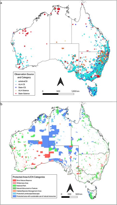
A. Stenhouse, T. Perry, F. Grützner et al. Global Ecology and Conservation 28 (2021) e01626
1. Introduction
Adequate assessment of the conservation status of many wildlife species in Australia and around the world is hampered by
limited information on abundance and distribution (Joppa et al., 2011; Pimm et al., 2014; Woinarski et al., 2015). Biodiversity
loss is increasing globally (Butchart et al., 2010) and on the Australian continent is likely worse than we currently realise (Wayne
et al., 2017; Woinarski et al., 2019). Historical causal factors of decline such as habitat loss, introduced predators and a range of
anthropogenic influences are now being exacerbated by changes to climate (Bradshaw, 2012; Urban, 2015; Woinarski et al.,
2019). In Australia, there have been multiple species extinctions (Woinarski et al., 2019, 2015) and 580 extant plant and animal
species are classified as endangered or critically endangered (IUCN, 2020). Many speciesʼ populations are in decline while the
status of many others remains unknown (IUCN, 2020).
Short-beaked echidnas (Tachyglossus aculeatus) are an iconic yet cryptic monotreme found throughout Australia in a wide
variety of habitats, ranging from coastal to mountain to desert (Brice et al., 2002; Grigg et al., 1989), with abundant and spatially
varying primary food sources of termites and ants (Abensperg‐Traun, 1994; Abensperg‐Traun and Steven, 1997). The Interna
tional Union for Conservation of Nature (IUCN) Red List rates the echidna as “Least Concern” as it is widely distributed in a broad
range of habitats, has few major threats and the population appears to be stable, although estimates range from 5 to 50 million
(Aplin et al., 2015). The IUCN status for widespread species is determined by historical trends in populations (IUCN, 2019),
which for cryptic species can be difficult to determine, particularly when they are broadly distributed (Black, 2020).
However, population trends are hard to determine without significant effort in collecting monitoring data. It is expensive
and difficult to survey and monitor wildlife species at large spatial scale (Crawford et al., 2020; Neate-Clegg et al., 2020).
Echidnas are particularly difficult to locate in the wild (Rismiller and McKelvey, 2003) and are not attracted by lures (Rismiller
and Grutzner, 2019). Additionally, their activity levels are affected by temperature – though usually diurnal, they tend to avoid
activity in extreme heat, so are often active at night in warmer climates and seasons (Brice et al., 2002; Clemente et al., 2016).
Traditional wildlife surveys and monitoring have usually been carried out by national and state government agencies, re
search organisations, non-governmental organisations and community groups. Survey efforts often focus on particular species
or groups of species which may act as ecosystem proxies or on particular, and often threatened, species or habitats. Long-term
monitoring does occur but usually at smaller spatial scale, as funding is limited and has competing priorities which change
over time.
There are few special efforts made to survey short-beaked echidna, and most observations are incidental, part of wider
general surveys or as a by-product of other targeted species surveys, often consisting of signs of presence, such as tracks or scat,
rather than actual species sightings. In addition, conducting formal surveys or obtaining sightings in remote areas is time-
consuming and expensive. These factors lead to a patchwork of geographic coverage in monitoring as well as low temporal
frequency, resulting in a lack of knowledge about current populations around Australia and thus difficulty in assessing how the
population may be changing over time.
On Kangaroo Island in South Australia, long-term studies of the local sub-species (Tachyglossus aculeatus multiaculeatus)
have shown population declines (Rismiller and Grutzner, 2019), resulting in the recent listing of this sub-species as “En
dangered” under national biodiversity conservation legislation (Department for Environment and Water DEW, 2017). The im
proved understanding of population status provided by more intensive studies raises questions about the IUCN classification of
the species Australia-wide. Impacts from habitat modification, invasive species such as fox and cats, climate change and human
population impacts combined with its low reproductive rate (Nicol and Andersen, 2007; Rismiller and McKelvey, 2000) may be
contributing to more widespread decline.
Citizen Science (CS) has been suggested as a practical way to determine broad-scale population trends (Devictor et al., 2010;
Dickinson et al., 2010; Hochachka et al., 2012) and has been rapidly expanding globally (Bonney et al., 2014; Follett and Strezov,
2015). This has been enabled by technological advances such as mobile phones with integrated cameras, GPS and easy-to-use
apps (Baker, 2016; Silvertown, 2009). These provide a platform for non-specialists to quickly and easily record incidental ob
servations that provide accurate and timely data. It is envisaged that CS contributions to biodiversity monitoring in Australia
will continue to increase, as community engagement is one of the three goals of Australia's Strategy for Nature from 2019 to
2030 (Commonwealth of Australia, 2019) aiming to fulfil Australia's international commitments under the Convention on
Biological Diversity (CBD or Aichi Biodiversity Targets) and the Sustainable Development Goals (SDGs) (United Nations
Development Program, 2018).
There have been two community-based CS echidna monitoring projects in Australia, both called echidnaWatch – one in
Queensland (https://wildlife.org.au/echidnawatch/) and one in South Australia (http://www.echidna.edu.au/monotremes/
echidna_watch.html). Both have used paper-based collection mechanisms supplemented by phoned-in and email reports.
However, these sometimes contain key metadata quality shortcomings, such as spatial inaccuracy, which can reduce its us
ability (Bayraktarov et al., 2019). In Queensland, these reports have been collated and uploaded to the State biodiversity re
pository but with delays, as no new records have been uploaded since 2016. The South Australian echidnaWatch recorded
sightings to its own database though updates have been delayed due to the obsolescence of the software used – and it has now
been superseded by our Echidna Conservation Science Initiative (echidnaCSI) project. For this study, we developed a mobile app
– echidnaCSI – to enable the public to easily submit incidental observations of this iconic species, with accurate, automatically
recorded metadata, such as location and date and time, and some additional observational details, such as size and activity.
One of the criticisms of CS data is that they are often biased (Mair et al., 2017; Silvertown et al., 2013), as citizen sightings
and records do not follow structured surveys and that this introduces spatial and temporal biases, amongst others, into the data.
2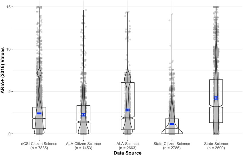
A. Stenhouse, T. Perry, F. Grützner et al. Global Ecology and Conservation 28 (2021) e01626
While this may substantially affect the usability of CS data for some purposes, improved technology can enhance the quality of
the data (Budde et al., 2017; Newman et al., 2012; Stenhouse et al., 2020). Scientific data can also be subject to biases, parti
cularly when aggregated from different sources over broad temporal and geographic scales (Beck et al., 2014; Boakes et al.,
2010; Piccolo et al., 2020). In this paper, we investigate some aspects of spatial bias by comparing our CS data to traditional
sources from Australian national and state biodiversity repositories.
Our aims in this paper are to investigate specific questions about the abundance and distribution of our echidna CS records
in relation to those from traditional sources stored in Australian national and state biodiversity repositories. 1: By using a
mobile app, can CS using a dedicated mobile app intensify and expand spatial coverage of a cryptic, yet widespread, species?
This could result in better baseline population information and enable improved assessment of population changes in the
future. 2: Are there differences in coverage in protected areas (PA) and non-protected lands between our echidnaCSI ob
servations and those from other data sources? PA are seen as a key solution for satisfying national and global commitments to
conserve biodiversity (Buckley et al., 2008), especially as climate refugia become even more vital for biodiversity protection
(Graham et al., 2019). Formal scientific surveys tend to focus on high-quality habitats that are often conserved in PAs. In
contrast, we expect to record more CS observations than scientific data sources in non-protected areas and from PA where the
general public is encouraged to visit and fewer from PA where access is more restricted. 3: Does geographic remoteness and
accessibility affect observation counts? As CS observations are often biased, we examine the geographic remoteness of echidna
observational records across Australia to assess differences between echidnaCSI and other sources. We expect to record fewer
observations from remote locations than traditional scientific data sources and more from locations with easier access.
2. Materials and methods
2.1. App development
The echidnaCSI app was developed using LiveCode (starting with version 8.1.5, www.livecode.org and www.livecode.com) –
an open-source, multi-platform development environment enabling rapid application development using one source code base
for multiple target devices. The app was compiled for both iOS and Android platforms and runs on mobile devices that can
provide location information, have a camera and a compatible Operating System (currently Android version 4.2 or later and iOS
10.0 or later).
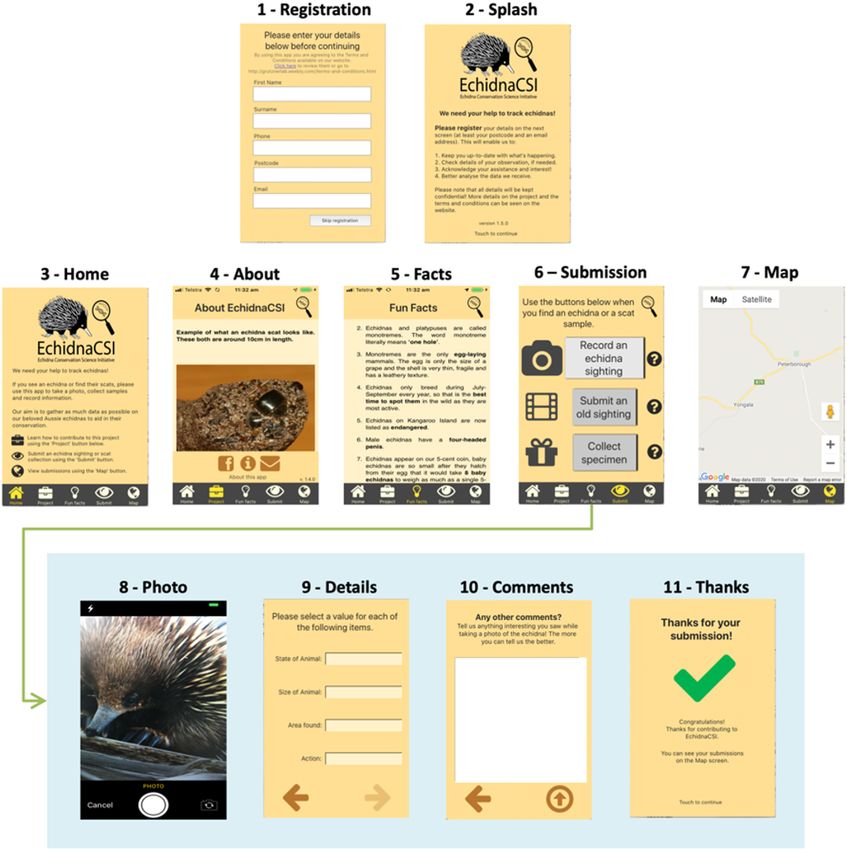
The app screen flow is illustrated in Fig. 1. After the user arrives at the Home screen, they can submit data by navigating to
the Submission screen and selecting one of three options: recording a current sighting, submitting a previously recorded photo
and thirdly, collecting a physical specimen.
To record a current sighting, the “Record an echidna sighting” button is touched. This starts the camera view, which enables
a photo to be taken immediately, while the echidna is in view. Once the photo has been taken, reviewed and accepted by the
user, the participant answers a series of questions using a series of dropdown fields to constrain and standardise the responses
(Table S1). These questions relate to this echidna's size, status (alive/dead), activity and location. Location data and date and
time are automatically saved along with some measures of location accuracy. On completing the Details screen questions, the
Comments screen allows the participant to enter free-text commentary to provide any further information that they deem
relevant. On completion, the data is uploaded directly to the project data repository (https://biocollect.ala.org.au/acsa/project/
index/8c3ae3b1-5342-40b4-9e72-e9820b7a9550) on the BioCollect portal at the Atlas of Living Australia (ALA). If network
access is unavailable this may fail, but all data is stored in the app and the next upload attempt will include any data not
previously successful. No network access is required to record an observation so remote use of the app is possible.
Photos taken at prior times and locations may also be submitted, provided they have accompanying location metadata. The
same process as above is followed once the photo has been accepted. Collection of physical specimens such as scats is also
possible and the participant is guided through the actual collection process after taking a photo to record location, date and time
details. Each participant’s observations are submitted to and identified in the ALA only by a Unique User ID (UUID) to ensure
privacy. Data is recorded on the device to a tab-delimited key-value pair text file with one observation per line (Table S2).
2.2. App in use – echidnaCSI
The echidnaCSI app was first released on 2 September 2017 and updated six times for iOS devices on the App Store and eight
times for Android devices via the Google Play platform. The most recent release is version 1.4.0 which was released on August
11, 2019 for iOS devices and for Android devices on August 12, 2019. A project website (https://grutznerlab.weebly.com/
echidna-csi.html) provides a central go-to point for project information including app download links. The project repository on
BioCollect at the ALA provides a web-based form interface to enter observations made without the app.
Community participation has been continually encouraged through the media including national and regional TV, news
paper and radio stations, social media such as Facebook (EchidnaCSI) and Instagram (echidna_csi), email updates to registered
participants and community outreach events (Perry et al., In preparation).
3
A. Stenhouse, T. Perry, F. Grützner et al.                                                                     Global Ecology and Conservation 28 (2021) e01626

                                      Fig. 1. Screen flow of the echidnaCSI app. Submissions take place in the bottom screens.

2.3. Data summary

   For this study, we have selected all echidna observations submitted to the echidnaCSI project between 01/09/2017 and 13/
08/2020 using the echidnaCSI app or the project web interface on BioCollect. We also downloaded all other available echidna
records from the ALA on 12/08/2020 (DOI: 10.26197/5f33a71948c4e) and all echidna records from the state governmental
repositories for NSW (14/09/2020), Victoria (14/09/2020), South Australia (09/09/2020), Queensland (11/09/2020), Western
Australia (15/09/2020), Tasmania (12/09/2020) and the Northern Territory (09/09/2020). We restricted the external datasets to
records from 01/09/2017 onwards to better compare to the data gathered in our project. Despite the difference in download
dates, there is only one extra record from the state systems in the period described. Some records were removed as a result of
data cleaning.
   Some state systems share data with the ALA (and vice-versa) so these two data sources are not independent of each other,
but the echidnaCSI data is independent of both, so we compare echidnaCSI data to ALA and then to state data separately. Further

                                                                                 4
A. Stenhouse, T. Perry, F. Grützner et al. Global Ecology and Conservation 28 (2021) e01626
Table 1
ARIA+ (2016) categorised values.
ARIA+ (2016) category ARIA+ (2016) values
Highly Accessible 0–0.20
Accessible > 0.20–2.40
Moderately Accessible > 2.40–5.92
Remote > 5.92–10.53
Very Remote > 10.53–15.00
details on data sources and filtering of these records for use in this study are provided in Supplementary information
(S1 Methods).
To analyse coverage within PA, we downloaded the Collaborative Australian Protected Areas Database (CAPAD) 2018
(Australian Government Department of Agriculture, Water and the Environment, 2019) which provides spatial and textual
information about national, state and private PA for Australia. This version includes 12,052 terrestrial PAs covering
151,787,501 ha (19.74%) of the Australian landmass (Department of Agriculture, Water and the Environment, 2020). For clas
sification of PA, we used the IUCN categories (Table S3) which are an internationally recognised standard and classify PA
according to their management objectives (Dudley et al., 2013).
To analyse the geographic distributions of observation locations we used the Accessibility and Remoteness Index of Australia
2016 Plus (ARIA+) (Hugo Centre for Population and Housing, 2020). ARIA+ is a continuously varying index of relative remoteness
for Australian locations with values ranging from 0 (high accessibility) to 15 (high remoteness). A nationally recognised measure
that has been used to derive the Australian Bureau of Statistics (ABS) Remoteness Area classification for Australia since 2001
(Taylor and Lange, 2016), the 1 km2 ARIA+ 2016 grid was used to assign ARIA+ scores to all of our observations. We subsequently
classified our observation’s ARIA+ scores into the ABS Remoteness Area categories (Australian Bureau of Statistics, 2018), as
indicated in Table 1.
2.4. Analysis
We classified the origin of data from the ALA and state systems as Citizen Science or Science on the basis of several attributes
(see Supplementary Info S1.1 for details). This resulted in five groups of data for analysis: echidnaCSI, which is all of CS origin;
ALA-CS data; ALA-Science data; State-CS data and State-Science data. We analysed for differences between echidnaCSI and the
other four groups in numbers of observations in PA and non-protected areas, and geographic distribution of observations, as
measured by the ARIA+ remoteness/accessibility index.
We used the QGIS vector analysis tools (QGIS Development Team, 2020) to determine if observations were contained in PA
and summarised and analysed the data using R. To test if source and science category groups had an effect on observation
counts in the PA IUCN categories, we used Pearson's chi-squared test with Cramer's V for effect size (Howell, 2011). We removed
the IUCN PA category "Not Assigned" as it contained too few observations. We compared observation counts for echidnaCSI to
those of ALA-CS and ALA-Sci and then compared echidnaCSI to State-CS and State-Sci observations separately, as ALA and State
observations are not completely independent – some data were shared between them.
We used the ARIA+ index to assess possible differences in geographic distribution between observations from our
echidnaCSI CS project and observations from the ALA and state systems, each split into CS and scientific data as above. We first
used the Shapiro–Wilk test of normality on each group. As all groups were not normally distributed, we used the non-para
metric Kruskal–Wallis test (Dodge, 2008) and Dunn's pairwise post-hoc test with the Benjamini–Hochberg adjustment method
to assess differences in distributions between the five observation groups.
Analyses were performed using RStudio version 1.2.5019 (R Core Team 2019) with R version 3.6.1 using the following
packages: data cleaning and preparation for analysis with tidyverse (Wickham et al., 2019), statistical analysis and graphs with
ggstatsplot (Patil, 2018), graphs with ggplot2 (Wickham, 2016) and maps with ggmap3 (Kahle and Wickham, 2013). Final maps
were prepared with QGIS 3.14 (QGIS Development Team, 2020).
3. Results
3.1. Data sources
3.1.1. EchidnaCSI
Observations were submitted using both the echidnaCSI app and the project web interface on BioCollect at the ALA. A total
of 8859 users registered the app, of which 2718 (app 1943; web 775) have submitted a total of 7835 observations of echidna
(app 6705; web 1130). The overall mean echidna observations per participant was 2.88 (app 3.45; web 1.46) and the median was
1 (app 2; web 1) (Table S4). The maximum total number of observations submitted by one participant over this study period
was 115 using the app and 107 using the web.
There were 7538 observations of living echidnas (94%) and 297 of dead echidnas (4%). The majority were of medium (55%) to
large (40%) size, with 130 (2%) young echidnas (puggles) recorded (Table S5). Most observations were made in bushland (34%),
5A. Stenhouse, T. Perry, F. Grützner et al. Global Ecology and Conservation 28 (2021) e01626
(caption on next page)
6A. Stenhouse, T. Perry, F. Grützner et al. Global Ecology and Conservation 28 (2021) e01626
Fig. 2. (continued)
Fig. 2. A) Echidna observations from all data sources; b) protected areas according to IUCN categories; c) distribution of ARIA+ (2016) accessibility/remoteness
categories across Australia.
along the roadside (26%) or in farmland (23%), with 856 (11%) in urban/backyard areas and 242 (3%) in coastal areas or along
waterways (Table S6). 83% (247/297) of dead echidna were recorded along the roadside. 54% were observed walking, 33%
digging and only 0.5% (42) observations of echidnas mating (Table S7).
Observations were recorded from every state and territory in Australia, with higher concentrations, as expected, around
more densely populated areas in NSW, Victoria and South Australia and fewer observations in sparsely populated areas.
3.1.2. ALA data
A total of 4116 echidna observations were recorded in the biodiversity repository at the ALA for our study period. Of these,
2663 were from Scientific sources and 1453 of CS origin (Table S8), with the main CS sources being iNaturalist (169), Ques
tagame (351) and individual uploads to BioCollect on the ALA. Most observations (2972) were recorded in NSW (Table S10).
3.1.3. State systems data
A total of 5476 echidna observations were contributed to the State biodiversity repositories during our study period, with
NSW and Victoria providing the majority (see Table S10 for details). Just over 50% (2786) were CS observations. Tasmania had a
particularly high proportion of CS records (93% – 259/278), as numerous roadkills were reported as part of an existing CS project
(Department of Primary IndustriesParks, 2020). A majority were also CS observations in NSW (66% – 2280/3438) where human-
wildlife conflicts are recorded in the form of Wildlife rehabilitation records (New South Wales Department of Environment,
Climate Change and Water, 2011).
3.1.4. Data summary
Combining data from all three data sources resulted in a total of 17,427 echidna observations (eCSI: 7835; ALA: 4116; state:
5476), with 12,074 (69%) from CS and 5353 (31%) from scientific sources (Table S8). There was much variation between States,
both in numbers of observations and in contributions from CS and science sources. These included totals of 8645 (CS: 4924, 57%;
Sci: 3721, 43%) in NSW, 4206 (CS: 3461, 82%; Sci: 745, 18%) in Victoria and 2352 (CS: 1757, 75%; Sci: 595, 25%) in South Australia
7A. Stenhouse, T. Perry, F. Grützner et al. Global Ecology and Conservation 28 (2021) e01626
(Tables S9 and S10). See Fig. 2 for overview maps of all observations (2a) with terrestrial protected areas (2b) and ARIA+ (2c)
categorised regions.
3.2. Observations in protected areas
There were 4162 observations (23.9%) recorded inside PAs, of which 1599 (38.4%) were from Citizen Science and 2563
(61.6%) from Scientific sources (Table 2). EchidnaCSI provided 24.6% of these, compared to 36.2% from the ALA and 39.2% from
the state systems. Citizen Science contributions inside PAs from the ALA were 9.7% of the total and from state systems just 4.1%
of the total PA observations. There were 13,265 observations (76.1% of all observations) recorded outside PAs, of which 10,475
(79%) were from Citizen Science and 2790 (21%) from Scientific sources. Approximately 13% of echidnaCSI observations were
made in PAs compared to over 36% of ALA and almost 30% of state system observations.
Table 2
Protected area observations.
Category IUCN description eCSI ALA State Total
CS Sci CS Sci
IA Strict Nature Reserve 77 40 167 9 311 604
IB Wilderness Area 10 7 33 0 54 104
II National Park 480 208 790 90 852 2420
III Natural Monument or Feature 266 56 30 11 53 416
IV Habitat/Species Management Area 120 63 68 39 55 345
V Protected Landscape/Seascape 20 11 2 7 9 49
VI Protected area with sustainable use of natural resources 51 19 12 15 124 221
NAS Not Assigned 0 0 1 0 2 3
Total PA 1024 404 1103 171 1460 4162
NA Not Protected 6811 1049 1560 2615 1230 13,265
Total 8859 1857 3766 2957 4150 21,589
When considering PA observations by IUCN category, the majority of observations were in "National Parks", followed by
"Strict Nature Reserves", "Natural Monument or Feature" and "Habitat/Species Management Area". Of particular note are the
large numbers of observations from Scientific sources in the state and ALA systems in the categories of "National Park" and
"Strict Nature Reserve". Also noteworthy is the contribution from echidnaCSI in the "Natural Monument or Feature" and
"Habitat/Species Management Area" categories and relatively poor contribution in the "Strict Nature Reserve" and "Wilderness
Area" categories. There was much variation in PA observations between States, with only two States having observations in
“Wilderness Areas”, where echidnaCSI provides only 10 observations out of a total of 104 across the whole country. For a
detailed breakdown of observations by IUCN category per state and data source see Table S12, and for observation counts by
IUCN category, State and CS/Science contributions to each see Table S13.
The results from testing the effect of data-source and science type on IUCN PA category using Pearson's chi-square test of in
dependence and post-hoc test using Cramer's V are presented in Table 3. A statistically highly significant association with moderate
effect is indicated overall for observation counts between echidnaCSI and ALA data sources (χ2 (14, N = 11,950) = 1516.71, p < 0.001,
Cramer's V = 0.25) and with moderate-strong effect between echidnaCSI and state data sources (χ2 (14, N = 13,309) = 3237.78,
p < 0.001, Cramer's V = 0.35).
Table 3
Pearson's chi-square test results for the independence of observation counts per PA category against data source.
Data sources DF Statistic p-value Cramer's V CI95% N
eCSI, ALA-CS, ALA-Sci 14 1516.71 1.19 e−315 0.25 [0.23,0.26] 11,950
eCSI, State-CS, State-Sci 14 3237.78 0 0.35 [0.33,0.36] 13,309
When comparing data sources within each PA category, a statistically highly significant difference with moderate effect on
observation counts is seen across all PA categories except for category V (Protected Landscape/Seascape) when comparing
echidnaCSI to ALA observations (Table S14) and all PA categories when comparing echidnaCSI to state observations (Table S15).
This suggests that the observation method and PA category are not independent and that the strength of this association varies
across PA categories. EchidnaCSI has markedly more observations in IUCN category III and non-protected areas, with noticeably
fewer in IUCN category IA, IB and II, with smaller differences in the other categories.
8A. Stenhouse, T. Perry, F. Grützner et al. Global Ecology and Conservation 28 (2021) e01626
3.3. Geographic distribution of observations
EchidnaCSI provided more observations in every ARIA+ category than both other data sources except for the “Very Remote”
category, where state systems provided 167 observations compared to 77 from echidnaCSI and 46 from the ALA. Further
splitting the data sources into Citizen Science and Science categories shows the significant contribution eCSI makes in all
categories of accessibility (Table 4).
Table 4
Observation counts by ARIA+ (2016) category, source and science category.
ARIA+ (2016) categories eCSI ALA State Total
CS CS Sci CS Sci
Highly Accessible (0.00–0.20) 1232 417 554 982 186 3371
Accessible (> 0.20–2.40) 3656 483 931 1369 816 7255
Moderately Accessible (> 0.24–5.92) 2017 429 497 383 939 4265
Remote (> 5.92–10.53) 853 101 658 50 584 2246
Very Remote (> 10.53–15.00) 77 23 23 2 165 290
Total 7835 1453 2663 2786 2690 17,427
The ARIA+ values from echidnaCSI have a higher mean (2.41 ± 2.43) than the other two CS groups but lower than the Science
groups. The State Science data are the most widely dispersed and with a higher ARIA+ mean of 4.23 ± 3.55 compared to
1.14 ± 1.48 for State CS data, while ALA Science data have a mean of 2.81 ± 2.71 compared with 2.23 ± 2.58 for ALA CS data, with
echidnaCSI remaining at 2.41 (Table 5). All group distributions are skewed with numerous outliers and bimodal characteristics
are indicated in some groups (Fig. 3).
The data source group had a highly significant moderate effect on geographical distribution of observations as indicated by
the Kruskal–Wallis test results (χ2 (4, N = 17,427) = 1789.40, p = 0.0, ε2 = 0.10). There are highly significant differences in the
geographic distribution of observations between echidnaCSI and the other four groups, except when comparing echidnaCSI to
ALA-Sci (p = 0.03) as shown by the post-hoc Dunn test with Benjamini-Hochberg correction (Table 6).
Table 5
ARIA+ value statistics by data source and category.
Source Category Mean Median SD Max IQR Count
eCSI Citizen Science 2.41 1.82 2.43 15.00 2.52 7835
ALA Citizen Science 2.23 1.39 2.58 14.62 3.25 1453
ALA Science 2.81 1.87 2.71 14.41 5.58 2663
State Citizen Science 1.14 0.61 1.48 14.12 1.76 2786
State Science 4.23 3.24 3.55 15.00 5.08 2690
4. Discussion
4.1. Mobile app use
The echidnaCSI app has provided an easy-to-use tool for members of the public to quickly and easily record opportunistic
sightings of echidna. A large number of participants have successfully submitted sightings, with some very enthusiastic par
ticipants using either the app or web interface regularly. This has resulted in almost doubling the number of echidna ob
servations across Australia over the study period, which should considerably improve the accuracy of future population
assessments by providing greater species presence data at wider spatial distribution than may be possible using traditional
methods. The retention of regular participants should prove useful for providing improved longitudinal data, enabling better
long-term analysis in certain areas.
Most observations from echidnaCSI were contributed by participants in the states of Victoria, New South Wales and South
Australia, which is different from the other two data sources which were dominated by contributions from New South Wales
(Table S10). This is probably due to the publicity that was generated for the project through both traditional and social media
channels, which provided a focal point for interest in this particular species, supported by the use of a dedicated app. This
resulted in echidnaCSI providing two to three times more observations than the other data sources in many states, apart from
New South Wales, which recorded a similar number of observations to echidnaCSI. Much higher observation numbers are
particularly noticeable in South Australia where the echidnaCSI project is based and more local events provided avenues for
community engagement and interest which supplemented the other engagement channels.
Utilising the ALA as a biodiversity repository provides multiple benefits. It provides a stable, central portal for storage and
access of observational data in standardised format which enables the wider use of these data for biodiversity research
(Theobald et al., 2015). It also provides a web interface that enables participants to supply observations recorded using devices
other than mobile phones. In contrast to the app, the web interface to the ALA requires users to register before allowing
9A. Stenhouse, T. Perry, F. Grützner et al. Global Ecology and Conservation 28 (2021) e01626
Fig. 3. Distribution and summary statistics of ARIA+ (2016) index for observations for each data source and Citizen Science/Science category.
Table 6
Statistical results from pairwise comparison of ARIA+ data by data source groups using the Kruskal–Wallis test with Dunn post-hoc test.
Group 1 Group 2 Dunn Statistic pFDR-corrected Sig
eCSI-Citizen Science ALA-Citizen Science 6.04 1.68 e−9 ***
eCSI-Citizen Science ALA-Science 2.12 0.03 *
eCSI-Citizen Science State-Citizen Science 27.38 2.54 e−164 ***
eCSI-Citizen Science State-Science 23.36 2.50 e−120 ***
ALA-Citizen Science ALA-Science 6.75 1.80 e−11 ***
ALA-Citizen Science State-Citizen Science 13.33 2.29 e−40 ***
ALA-Citizen Science State-Science 21.34 9.94 e−101 ***
ALA-Science State-Citizen Science 24.04 3.36 e−127 ***
ALA-Science State-Science 17.36 2.96 e−67 ***
State-Citizen Science State-Science 41.66 0 ***
contributions, which may be a barrier to use (Jay et al., 2016; Martin et al., 2016). The web interface does not automatically
record location, date and time as the app does, and thus may introduce some errors when these are entered manually. It does
record these from the metadata of an uploaded photo, if available, however. Nonetheless, it provides another very useful
capability with little effort for the project team and resulted in a significant contribution in numbers of users and observations.
The app could be improved by better integration with the ALA. As participants using the app are assigned a Unique User
Identifier (UUID) and are not automatically registered on the ALA, they cannot easily find their own observations on the ALA
website. Ideally this should be improved so that the interface between systems is as seamless as possible, while preserving the
low barrier-to-use of the app. Additionally, being able to see both their own and others' contributions from inside the app as
well as online, and to be able to share these easily, would likely improve participants' engagement with the app and potentially
increase the number of people using it.
10A. Stenhouse, T. Perry, F. Grützner et al. Global Ecology and Conservation 28 (2021) e01626
4.2. Protected areas
EchidnaCSI was successful in providing more observations in PA than from other CS sources as well as a large increase in
observations in non-protected areas overall. There were significant differences in the number of observations in the varying PA
IUCN categories. In "Strict Nature Reserves", human visitation, use and impacts are strictly controlled to ensure the protection of
conservation values, so it is not surprising there were fewer CS observations in these PA. "Wilderness Areas" provide for re
stricted public access but aim to preserve the area's ecological integrity and should remain undisturbed by significant human
activity, so CS observations in these areas are interesting, as visitor access is more limited and more likely to be confined to
those with the skills and equipment to survive unaided (Dudley et al., 2013). PA where public access is encouraged, however,
showed significantly higher numbers of observations from echidnaCSI, as might be expected. Contributing factors to this may
include ease of access and the possibility that science-based studies prefer areas with less human disturbance. EchidnaCSI
provided the majority of CS observations in all PA categories, which indicates how successful this project has been at attracting
participation.
There was much variation in PA observations among States. For example, in the Northern Territory there were a total of 41
observations recorded in the State repository and these were all from camera traps. New South Wales had few PA observations
provided by CS, whereas in Victoria and South Australia echidnaCSI provided almost as many sightings as were recorded by the
State scientific sources, indicating the value of this project. This may be explained by the abundance of PA allowing public
access, such as IUCN II–V, close to heavily populated areas of Adelaide in South Australia and Melbourne in Victoria. Population
size probably also plays a role, which would also affect the numbers of governmental and other organisations monitoring
biodiversity.
There are many challenges associated with managing PA for effective biodiversity conservation, both in Australia (Buckley
et al., 2008; Watson et al., 2011; Woinarski et al., 2011) and worldwide (Cazalis et al., 2020; Gaston et al., 2006; Geldmann et al.,
2019; Watson et al., 2014). Improving monitoring methods will surely involve utilising the public in recording incidental ob
servations, as in echidnaCSI, complemented by using more structured methods performed by professionals and also by citizen
scientists (Kelling et al., 2019; Pescott et al., 2015). Access to PA by the public can also be detrimental to biodiversity (Xavier da
Silva et al., 2018) so care must be taken when assessing monitoring methods and conservation management.
4.3. Geographic distribution by remoteness areas
EchidnaCSI provided more observations in all categories of remote areas of Australia than other sources except for Very
Remote regions where State Scientific observations are most numerous. There are clear differences in remoteness between
scientific and CS observations from State systems and this difference is less in ALA data. This smaller difference in ALA data may
be due to possible misclassification of some data as CS, where it appears that data transfer between systems may have occurred
without data sources being correctly recorded. The State systems included better indications of data sources enabling easier CS/
Science classification which resulted in the clearer differences.
Except for Highly Accessible areas, the number of observations decreases with increased remoteness, both overall and for
echidnaCSI. i.e. there are fewer observations in more remote areas. As Highly Accessible areas are very urbanised, it should not
be too surprising that there are fewer observations in this category. The large increase in observations in Accessible areas may
be explained by the availability of suitable habitat areas combined with their proximity to populated areas. Very large areas of
Australia are classified as Remote or Very Remote and there are few observations in these areas. There is a need for more data
from these remote areas and though some exist, these are often in siloed repositories where the data are slow to be shared more
widely, if at all.
Small geographic clusters of scientific observations in Remote and Very Remote areas can be seen in NW, N and SE Australia
(Fig. 2a). These observations from the Western Australian, Northern Territory and Victorian state systems have observation type
recorded and the majority of these are camera trap (CT) images. Automated recording technologies such as CT and audio
recorders have great potential to increase species observations in remote areas. As they can operate throughout the day and
night, they may increase the chances of recording echidna activity in warmer climates where echidna may be more active at
night when other methods are less likely to detect them. This uninterrupted usage combined with their suitability for remote
locations indicates CT to be a potentially complementary method to CS/echidnaCSI observations (Santangeli et al., 2020). As the
climate continues to change, this may become a bigger issue as both humans and species such as the echidna adapt their
behaviours to avoid temperature extremes (Graham et al., 2019; Heller and Zavaleta, 2009; Mackey et al., 2008; Synes
et al., 2020).
EchidnaCSI has provided very good coverage of most regions apart from Very Remote areas. Given the lack of funding for
environmental research in Australia and the expense of remote fieldwork, to increase coverage in these regions may require
increased engagement with inhabitants of remoter regions, such as indigenous groups and others who temporarily visit these
areas, such as mine workers and tourists. Payments for ecosystem services, which are increasingly used to reward landowners
for preserving ecological-beneficial habitats and features, could be extended to cover payments for biodiversity monitoring
services here in Australia (Rawlins and Westby, 2013; Tuanmu et al., 2016), though this should be used cautiously (Sommerville
et al., 2011; van Berkel et al., 2018) as participants' continued engagement often stems from intrinsic science- and conservation-
related motivations (Larson et al., 2020). The intensification of observations provided by echidnaCSI could also be used to
stimulate CS activity in areas with fewer observations and would be made more useful by also recording CS search paths
11A. Stenhouse, T. Perry, F. Grützner et al. Global Ecology and Conservation 28 (2021) e01626
(Stenhouse et al., 2020). Gaps in desired observational coverage can then be prioritised for professional surveying, if necessary
(Tulloch et al., 2013).
Disparate state data standards mean data usability is reduced. This could be overcome by ensuring data is uploaded to a
national system that provides ease of use and access to consistent and standard format data for local and global researchers,
enabling more rapid evaluations of current biodiversity. In Australia, the ALA provides a national biodiversity repository but it
appears that some state systems are slow to integrate with it and that this integration sometimes lacks in detail, leading to
difficulties in determining data sources. Though funding is limited and policy conflicts may exist, it would be highly beneficial to
more fully utilise the services that the ALA provides (Salle et al., 2016). Its value is being increasingly recognised around the
world as the increasing uptake of the ALA software by other countries shows (https://living-atlases.gbif.org/).
The integration of a variety of monitoring methods can lead to more effective monitoring with benefits for biodiversity and
society. By utilising both scientific and community sources, programme ownership and resilience may be broadened and
societal benefits enhanced (Kühl et al., 2020).
5. Conclusions
The echidnaCSI app provided an easy-to-use system for citizen scientists to quickly provide accurate, vouchered data in a
usable form to the project repository on the national biodiversity database. EchidnaCSI has substantially increased the spatial
and temporal intensity of echidna observations around Australia since starting in September 2017. EchidnaCSI has provided
comparable geographic distribution to other existing biodiversity surveys and databases at all levels of remoteness as measured
by the ARIA+ index of accessibility, except for the Very Remote category. Some protected areas are also less covered by CS,
indicating the value of professional surveys in these areas, particularly in PAs where public access is discouraged. While large
gaps in geographic coverage for the Australian Short beaked echidna remain, this study indicates that CS programmes can
provide good observational data for a cryptic species at large scale and can highlight areas where scientific monitoring may
provide even greater value. We plan to continue the refinement and promotion of the echidnaCSI project and app in order to
increase the geographic and temporal extents of the data. This may enable further collaborative studies with ecologists and
environmental scientists to address specific questions related to the ecology, distribution and conservation of this species and to
detect the longer-term trends required to better evaluate the conservation status for this species on the Australian mainland.
Data Availability
EchidnaCSI is a free mobile app available for Android https://play.google.com/store/apps/details?id=com.scruffmonkey.
echidnaCSI) and on iOS (https://itunes.apple.com/au/app/echidnacsi/id1260820816). Data is available for download from the
DOIs and websites listed in Supplementary information S2. Application code is available on FigShare at DOI: 10.25909/14528367
and Github at https://github.com/alanstenhouse/echidnaCSI-app.
Declaration of Competing Interest
The authors declare that they have no known competing financial interests or personal relationships that could have
appeared to influence the work reported in this paper.
Acknowledgements
AS and TP were supported by Australian Government Research Training Program Scholarships. LPK is supported by the
Singapore National Research Foundation (NRF-RSS2019-007). FG is supported by an ARC Future Fellowship (FT160100267).
Thanks to other members of the echidnaCSI team: Isabella Wilson, Ella West, Ima Perfetto, Michelle Coulson and Peggy
Rismiller. Jarrod Lange from the Hugo Centre for Population and Housing at the University of Adelaide kindly provided assis
tance and advice on evaluating geographic distribution using ARIA+ (2016) and extracted ARIA+ values for our observations.
Many thanks to Peter Brenton and colleagues from the Atlas of Living Australia for assistance and advice throughout the project;
and also to our app testers and especially all the participants in echidnaCSI who submitted observations. Human ethics
clearance for the echidnaCSI project was approved by the University of Adelaide (HREC-2019-156).
Authors' contributions
All authors conceived the ideas and designed the study; AS developed the software and did the data analysis; AS, ML and LPK
led the writing of the manuscript. All authors contributed critically to the drafts and gave final approval for publication.
Appendix A. Supplementary information
Supplementary data associated with this article can be found in the online version at doi:10.1016/j.gecco.2021.e01626.
12A. Stenhouse, T. Perry, F. Grützner et al. Global Ecology and Conservation 28 (2021) e01626
References
Abensperg‐Traun, M., 1994. The influence of climate on patterns of termite eating in Australian mammals and lizards. Aust. J. Ecol. 19, 65–71. https://doi.org/10.
1111/j.1442-9993.1994.tb01544.x
Abensperg‐Traun, M., Steven, D., 1997. Ant- and termite-eating in Australian mammals and lizards: a comparison. Aust. J. Ecol. 22, 9–17. https://doi.org/10.1111/j.
1442-9993.1997.tb00637.x
Aplin, K., Dickman, C, Salas, L., Helgen, K., 2015. IUCN Red List of Threatened Species: Tachyglossus aculeatus. [WWW Document]. IUCN Red List of Threatened
Species. URL: ⟨https://www.iucnredlist.org/en⟩. (Accessed 25 October 2020).
Australian Bureau of Statistics, 2018. Australian Statistical Geography Standard (ASGS): Volume 5 – Remoteness Structure, July 2016. [WWW Document]. URL:
⟨https://www.abs.gov.au/ausstats/abs@.nsf/mf/1270.0.55.005?⟩. OpenDocument (Accessed 18 January 2021).
Australian Government Department of Agriculture, Water and the Environment, 2019. Collaborative Australian Protected Areas Database (CAPAD) 2018,
Commonwealth of Australia 2019. URL: ⟨https://www.environment.gov.au/fed/catalog/search/resource/details.page?uuid=%7B4448CACD-9DA8-43D1-
A48F-48149FD5FCFD%7D⟩. (Accessed 17 September 2020).
Baker, B., 2016. Frontiers of citizen science: explosive growth in low-cost technologies engage the public in research. BioScience 66, 921–927. https://doi.org/10.
1093/biosci/biw120
Bayraktarov, E., Ehmke, G., O’Connor, J., Burns, E.L., Nguyen, H.A., McRae, L., Possingham, H.P., Lindenmayer, D.B., 2019. Do big unstructured biodiversity data
mean more knowledge? Front. Ecol. Evol. 6. https://doi.org/10.3389/fevo.2018.00239
Beck, J., Böller, M., Erhardt, A., Schwanghart, W., 2014. Spatial bias in the GBIF database and its effect on modeling species’ geographic distributions. Ecol. Inform.
19, 10–15. https://doi.org/10.1016/j.ecoinf.2013.11.002
Black, S.A., 2020. Assessing presence, decline, and extinction for the conservation of difficult-to-observe species. In: Angelici, F.M., Rossi, L. (Eds.), Problematic
Wildlife II: New Conservation and Management Challenges in the Human-Wildlife Interactions. Springer International Publishing, Cham, pp. 359–392.
https://doi.org/10.1007/978-3-030-42335-3_11
Boakes, E.H., McGowan, P.J.K., Fuller, R.A., Chang-qing, D., Clark, N.E., O’Connor, K., Mace, G.M., 2010. Distorted views of biodiversity: spatial and temporal bias in
species occurrence data. PLOS Biol. 8, 1000385. https://doi.org/10.1371/journal.pbio.1000385
Bonney, R., Shirk, J.L., Phillips, T.B., Wiggins, A., Ballard, H.L., Miller-Rushing, A.J., Parrish, J.K., 2014. Next steps for citizen science. Science 343, 1436–1437.
https://doi.org/10.1126/science.1251554
Bradshaw, C.J.A., 2012. Little left to lose: deforestation and forest degradation in Australia since European colonization. J. Plant Ecol. 5, 109–120. https://doi.org/
10.1093/jpe/rtr038
Brice, P.H., Grigg, G.C., Beard, L.A., Donovan, J.A., 2002. Patterns of activity and inactivity in echidnas (Tachyglossus aculeatus) free-ranging in a hot dry climate:
correlates with ambient temperature, time of day and season. Aust. J. Zool. 50, 461–475. https://doi.org/10.1071/zo01080
Buckley, R., Robinson, J., Carmody, J., King, N., 2008. Monitoring for management of conservation and recreation in Australian protected areas. Biodivers.
Conserv. 17, 3589–3606. https://doi.org/10.1007/s10531-008-9448-7
Budde, M., Schankin, A., Hoffmann, J., Danz, M., Riedel, T., Beigl, M., 2017. Participatory sensing or participatory nonsense? Mitigating the effect of human error
on data quality in citizen science. In: Proceedings of the ACM Interactive, Mobile, Wearable and Ubiquitous Technologies, 1, pp. 39:1–39:23. ⟨https://doi.org/
10.1145/3131900⟩.
Butchart, S.H.M., Walpole, M., Collen, B., Strien, A., van, Scharlemann, J.P.W., Almond, R.E.A., Baillie, J.E.M., Bomhard, B., Brown, C., Bruno, J., Carpenter, K.E., Carr,
G.M., Chanson, J., Chenery, A.M., Csirke, J., Davidson, N.C., Dentener, F., Foster, M., Galli, A., Galloway, J.N., Genovesi, P., Gregory, R.D., Hockings, M., Kapos, V.,
Lamarque, J.-F., Leverington, F., Loh, J., McGeoch, M.A., McRae, L., Minasyan, A., Morcillo, M.H., Oldfield, T.E.E., Pauly, D., Quader, S., Revenga, C., Sauer, J.R.,
Skolnik, B., Spear, D., Stanwell-Smith, D., Stuart, S.N., Symes, A., Tierney, M., Tyrrell, T.D., Vié, J.-C., Watson, R., 2010. Global biodiversity: indicators of recent
declines. Science 328, 1164–1168. https://doi.org/10.1126/science.1187512
Cazalis, V., Princé, K., Mihoub, J.-B., Kelly, J., Butchart, S.H.M., Rodrigues, A.S.L., 2020. Effectiveness of protected areas in conserving tropical forest birds. Nat.
Commun. 11, 4461. https://doi.org/10.1038/s41467-020-18230-0
Clemente, C.J., Cooper, C.E., Withers, P.C., Freakley, C., Singh, S., Terrill, P., 2016. The private life of echidnas: using accelerometry and GPS to examine field
biomechanics and assess the ecological impact of a widespread, semi-fossorial monotreme. J. Exp. Biol. 219, 3271–3283. https://doi.org/10.1242/jeb.143867
Commonwealth of Australia, 2019. Australia’s Strategy for Nature 2019–2030.
Crawford, B.A., Olds, M.J., Maerz, J.C., Moore, C.T., 2020. Estimating population persistence for at-risk species using citizen science data. Biol. Conserv. 243,
108489. https://doi.org/10.1016/j.biocon.2020.108489
Department for Environment and Water (DEW), 2017. Kangaroo Island Short-Beaked Echidna. URL: ⟨https://landscape.sa.gov.au/ki/plants-and-animals/native-
animals/short-beaked-echidna⟩. (Accessed 25 October 2020).
Department of Agriculture, Water and the Environment, 2020 CAPAD: Protected Area Data. URL: ⟨https://www.environment.gov.au/land/nrs/science/capad⟩.
(Accessed 19 October 2020).
Devictor, V., Whittaker, R.J., Beltrame, C., 2010. Beyond scarcity: citizen science programmes as useful tools for conservation biogeography. Divers. Distrib. 16,
354–362. https://doi.org/10.1111/j.1472-4642.2009.00615.x
Dickinson, J.L., Zuckerberg, B., Bonter, D.N., 2010. Citizen science as an ecological research tool: challenges and benefits. Annu. Rev. Ecol. Evol. Syst. 41, 149–172.
https://doi.org/10.1146/annurev-ecolsys-102209-144636
Dodge, Yadolah, 2008. Kruskal-Wallis test. The Concise Encyclopedia of Statistics. Springer New York, New York, NY, pp. 288–290. https://doi.org/10.1007/978-0-
387-32833-1_216
Department of Primary Industries, Parks, Water and Environment, Tasmania, 2020. Roadkill Project. URL: ⟨https://dpipwe.tas.gov.au/wildlife-management/
save-the-tasmanian-devil-program/about-the-program/roadkill-project⟩. (Accessed 21 October 2020).
Dudley, N., Shadie, P., Stolton, S., 2013. Guidelines for Applying Protected Area Management Categories Including IUCN WCPA Best Practice Guidance on
Recognising Protected Areas and Assigning Management Categories and Governance Types.
Follett, R., Strezov, V., 2015. An analysis of citizen science based research: usage and publication patterns. PLOS ONE 10, 0143687. https://doi.org/10.1371/
journal.pone.0143687
Gaston, K.J., Charman, K., Jackson, S.F., Armsworth, P.R., Bonn, A., Briers, R.A., Callaghan, C.S.Q., Catchpole, R., Hopkins, J., Kunin, W.E., Latham, J., Opdam, P.,
Stoneman, R., Stroud, D.A., Tratt, R., 2006. The ecological effectiveness of protected areas: the United Kingdom. Biol. Conserv. 132, 76–87. https://doi.org/10.
1016/j.biocon.2006.03.013
Geldmann, J., Manica, A., Burgess, N.D., Coad, L., Balmford, A., 2019. A global-level assessment of the effectiveness of protected areas at resisting anthropogenic
pressures. PNAS 116, 23209–23215. https://doi.org/10.1073/pnas.1908221116
Graham, V., Baumgartner, J.B., Beaumont, L.J., Esperón-Rodríguez, M., Grech, A., 2019. Prioritizing the protection of climate refugia: designing a climate-ready
protected area network. J. Environ. Plan. Manag. 62, 2588–2606. https://doi.org/10.1080/09640568.2019.1573722
Grigg, G.C., Beard, L.A., Augee, M.L., 1989. Hibernation in a monotreme, the echidna (Tachyglossus aculeatus). Comp. Biochem. Physiol. A Comp. Physiol. 92,
609–612. https://doi.org/10.1016/0300-9629(89)90375-7
Heller, N.E., Zavaleta, E.S., 2009. Biodiversity management in the face of climate change: a review of 22 years of recommendations. Biol. Conserv. 142, 14–32.
https://doi.org/10.1016/j.biocon.2008.10.006
Hochachka, W.M., Fink, D., Hutchinson, R.A., Sheldon, D., Wong, W.-K., Kelling, S., 2012. Data-intensive science applied to broad-scale citizen science. Trends
Ecol. Evol. Ecol. Evolut. Inform. 27, 130–137. https://doi.org/10.1016/j.tree.2011.11.006
Howell, D.C., 2011. Chi-square test: analysis of contingency tables. In: Lovric, M. (Ed.), International Encyclopedia of Statistical Science. Springer Berlin
Heidelberg, Berlin, Heidelberg, pp. 250–252. https://doi.org/10.1007/978-3-642-04898-2_174
13You can also read