Gaussian mixture analysis of basic meteorological parameters: Temperature and relative humidity
←
→
Page content transcription
If your browser does not render page correctly, please read the page content below
Tecnología en marcha, Edición especial 2020
         6th Latin America High Performance Computing Conference (CARLA)                              5

     Gaussian mixture analysis of
 basic meteorological parameters:
Temperature and relative humidity
              Análisis de mixturas gaussianas de
             parámetros meteorológicos básicos:
                 Temperatura y humedad relativa
   Mariela Abdalah-Hernández1, Javier Rodríguez-Yáñez2,
                             Daniel Alvarado-González3

                  Abdalah-Hernández, M; Rodríguez-Yáñez, J; Alvarado-Gon-
                    zález, D. Gaussian mixture analysis of basic meteorological
                 parameters: Temperature and relative humidity. Tecnología en
                 Marcha. Edición especial 2020. 6th Latin America High Perfor-
                            mance Computing Conference (CARLA). Pág 5-12.

                                              https://doi.org/10.18845/tm.v33i5.5068

         1   Research assistant. National Advanced Computing Collaboratory, National Center
             for High Technology. Chemical Engineering student. Chemical Engineering School,
             University of Costa Rica. Costa Rica. Email: mariela.abdalah@ucr.ac.cr.
                 https://orcid.org/0000-0002-9790-2689
         2   Master of Environment, Chemical Engineer and researcher. Urban Ecology Laboratory,
             Universidad Estatal a Distancia. Costa Rica. Email: jrodriguezy@uned.ac.cr.
                 https://orcid.org/0000-0001-5539-3153
         3   Master of Computer Science and researcher. National Advanced Computing Collabo-
             ratory, National Center for High Technology. Costa Rica. Email: dalvarado@cenat.ac.cr.
                 https://orcid.org/0000-0003-3290-690X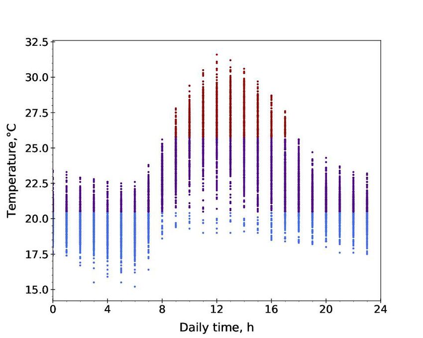
Tecnología en marcha, Edición especial 2020
6        6th Latin America High Performance Computing Conference (CARLA)

    Keywords
    Temperature; relative humidity; Gaussian mixtures; meteorology.

    Abstract
    Gaussian mixture modelling was applied to describe the annual distribution of two important
    meteorological variables, temperature and relative humidity, inside the Costa Rican Central Valley
    from 2010 to 2017. A fixed number of components of Gaussian mixtures were used to fit data to
    a general mixture curve that represented data behavior throughout the year, this was performed
    through specific functions of Scikit-learn and SciPy libraries of Python language. Low values
    of approximation error were obtained when modelling temperature data and the relationship
    between its distribution and hourly variability was observed, finding high values around noon.
    For relative humidity, the Gaussian mixture model presented issues when fitting values greater
    than 90 %, as a result of this variable saturation limit at 100 %. The relationship with time was
    not clearly determined due to the many mixture components used to model, but a tendency of
    low values between the late morning and early afternoon was visualized. Iterative minimization
    of the error was considered as a future approach to achieve a better fit with Gaussian mixtures
    of these and other meteorological variables.

    Palabras clave
    Temperatura; humedad relativa; mixtura gaussiana; meteorología.

    Resumen
    Se aplicó el modelado por mixturas gaussianas para describir la distribución anual de dos
    variables meteorológicas importantes, temperatura y humedad relativa, dentro del Valle Central
    de Costa Rica desde el 2010 hasta el 2017. Se utilizó un número fijo de componentes gaussianas
    para ajustar los datos a una curva de mixtura general que representara el comportamiento
    durante todo el año, esto se realizó a través de funciones específicas de las bibliotecas Scikit-
    learn y SciPy del lenguaje Python. Al modelar los datos de temperatura se obtuvieron valores
    bajos del error de aproximación y se observó una relación entre su distribución y la variabilidad
    horaria, estableciendo altas temperaturas alrededor del mediodía. Para la humedad relativa,
    el modelo de mixturas gaussianas presentó problemas en el ajuste de valores mayores al 90
    %, como resultado del límite de saturación de esta variable en el 100 %. La relación respecto
    al tiempo no fue claramente determinada debido a la cantidad de componentes de la mixtura
    usadas para modelar la humedad relativa, pero se apreció una tendencia de valores bajos entre
    el final de la mañana e inicios de la tarde. La minimización iterativa del error fue considerada
    como una aproximación futura para alcanzar un mejor ajuste con mixturas gaussianas para
    estas y otras variables meteorológicas.

    Introduction
    The region with the highest population and anthropogenic activity concentration in Costa Rica
    is the Central Valley. This is the reason why it is necessary to have a more accurate weather
    model for this area. Meteorological data analysis helps to understand climate behavior, the way
    it changes and how it affects human activity. This work is encompassed by a larger project that
    pretends to study the effects of contamination on the climate and on man-made structures, mainly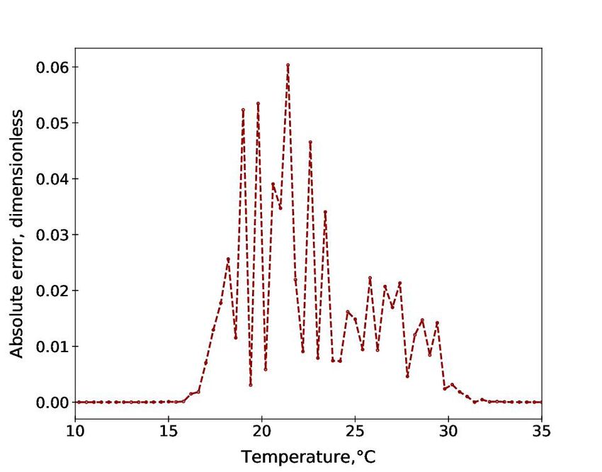
Tecnología en marcha, Edición especial 2020
                               6th Latin America High Performance Computing Conference (CARLA)           7

focusing on the corrosion of metallic structures. In this first stage, the main objective is to model
the distribution of temperature and relative humidity with Gaussian mixtures. Visualizing these
distributions will allow to improve the models for weather forecast, and even more importantly,
pollutant transport and particle deposition [1], [2].
These parameters were chosen because they are included inside of the typical meteorological
measures in all climatic stations, which means that there is a large amount of data available for
these variables (over 95 % of the annual data from the year 2010 to 2017). Additionally, they have
a direct relationship with the subject of corrosion [3], [4]. It is generally considered that relative
humidity and temperature affect corrosion when having values above 80 % and 0 °C [1], [2], [3].
By isolating these conditions per area, it could be determined which regions could have higher
corrosion levels in order to take it into account for the construction of metallic structures.
The main focus of this work was on the western part of the valley, limited to the northwest by the
Central Volcanic Mountain Range, to the east by the hills of Ochomogo and to the southwest by
the Talamanca Mountain Range [5].

Methodology
The selected parameters were temperature, which is a continuous function with no bounds, and
relative humidity, bounded between 0 % and 100 %. These data were obtained from weather
stations all around the Central Valley. For simplicity, in this work only three representative weather
stations were taken, two from opposite sides within the valley (northwest, and southwest) and
one located in the mountains.
The first step of the analysis consisted in generating visualizations of the frequency of values for
each parameter. Histograms were made where each category size corresponded to a band of
1 °C for temperature and 1 % for humidity. Gaussian mixture modelling was performed to obtain
a set of curves to approximate the real data in order to study the behavior throughout the year.
Also, the absolute error was calculated as the difference between the value of the approximation
function and the real frequency or density value. This error was used as a guidance to modify the
parameters of the mixture modelling function and the number of components, in order to achieve
a higher accuracy with the model. Time series was plotted, differentiating the points according
to the ranges determined by the means of the mixture components.
Calculations were performed with Python 3, Pandas, SciPy and Scikit-learn, specifically the
sklearn.mixture for the process of representing with Gaussian curves. The Pandas library was
used to manipulate the large amount of data, distributed among different files and provided by
the National Meteorological Institute of Costa Rica.

Results and discussion
In general, it was simpler to model temperature because there was not a maximum physical limit
in this variable. A good level of approximation was obtained utilizing a couple of Gaussians, as
it is shown in Figure 1. Errors found in the approximation curves were low, according to Figure
2, demonstrating the acceptable precision of the modelling.
A relationship between time series, represented as hours of the day, and the components was
observed too. The value of the mean of each Gaussian sets the limit of each colored zone in
Figure 3, were the purple zone corresponds to the overlapping area between both components.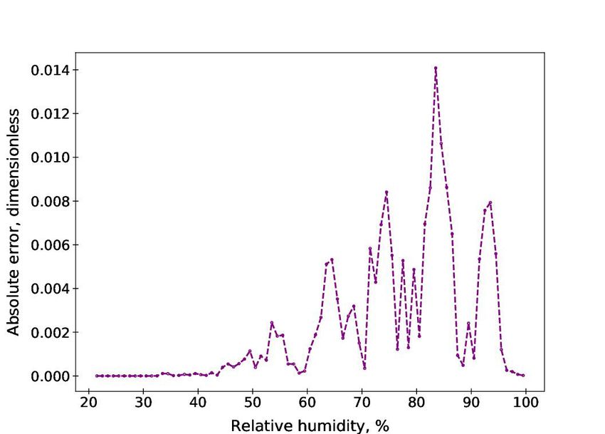
Tecnología en marcha, Edición especial 2020
8        6th Latin America High Performance Computing Conference (CARLA)

      Figure 1. Temperature density with a Gaussian mixture approximation in a station located in the northwest of the
                                                         valley.

     Figure 2. Error of the Gaussian mixture modelling of temperature in a station located in the northwest of the valley.

    Data of the first half of the first curve in Figure 1 was below 20.5 °C (light blue region in Figure
    3) and occurred around the morning and the afternoon. As it was expected, values above 25.5
    °C or the second half of the second curve, were measured around noon (red region) between
    09 h and 17 h.
    Relative humidity distributions were more complicated to model, this was because it was
    necessary to consider multiple curves in the mixture and due to the saturation value. The above
    generated issues when fitting cases where the frequency of data above 90 % was higher. For
    this range of values the error increased. This can be shown in Figures 4 and 5.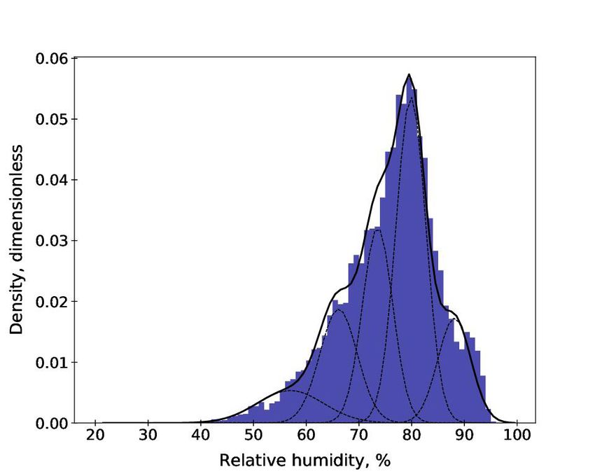
Tecnología en marcha, Edición especial 2020
                                   6th Latin America High Performance Computing Conference (CARLA)                     9

     Figure 3. Temperature distribution throughout the day in a station located in the northwest of the valley.

Figure 4. Relative humidity density with a Gaussian mixture approximation in a station located in the mountains of
                                                   the valley.

 Figure 5. Error of the Gaussian mixture modelling of relative humidity in a station located in the mountains of the
                                                      valley.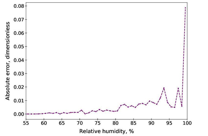
Tecnología en marcha, Edición especial 2020
10 6th Latin America High Performance Computing Conference (CARLA)
As can be seen in Figure 6, the achieved fit in other stations with lower humidity values was better
in comparison with the situation in the mountains. Figure 7 shows that absolute error was lower
in relative humidity than in temperature for this case, but this was obtained as a consequence of
requiring more approximation curves for an acceptable model, making the interpretation difficult.
Figure 6. Relative humidity density with a Gaussian mixture approximation in a station located in the southwest of
the valley.
Figure 7. Error of the Gaussian mixture modelling of relative humidity in a station located in the southwest of the
valley.
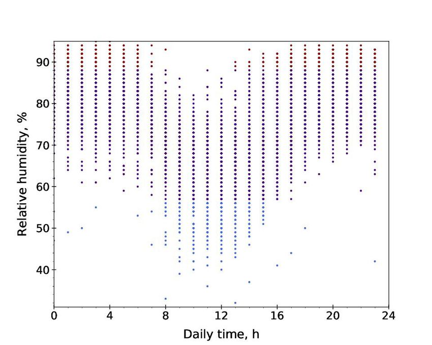
Analyzing time series, the quantity of components made the relationship unclear. However,
taking only the first and the last components the Figure 8 was obtained. The first half of the first
Gaussian was below 55 % approximately (light blue region), while high values in the second
part of the last curve were above 89 % (red region). Intermediate data located inside the other
components is grouped inside the purple area. In general terms, it was observed that low values
occurred between 08 h and 15 h.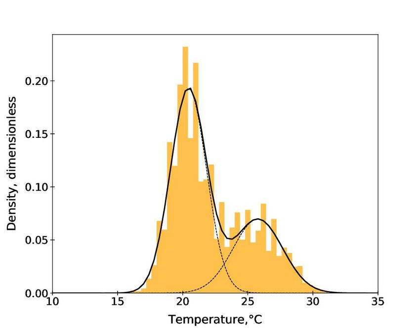
Tecnología en marcha, Edición especial 2020
                                       6th Latin America High Performance Computing Conference (CARLA)                   11

      Figure 8. Relative humidity distribution throughout the day in a station located in the southwest of the valley.

Conclusions
The approximation with Gaussian mixtures gave acceptable results for temperature, but
presented problems when modelling relative humidity near the 100 % value. The iterative
minimization of the error was an adequate strategy to visualize the issues with fitting relative
humidity, therefore it can be used with another techniques to improve modelling of this and other
variables. The subject of lack of precision near the saturation limit in relative humidity still has
to be solved. On the other hand, for temperature a good relationship between the distribution
and time series was found, while for relative humidity this was not clearly established due to the
number of components.
Modelling meteorological parameters with multiple Gaussians allows to notice associations with
time. These simplified models are fundamental for the development of subsequent models or
more complex dispersion algorithms. An example is the dispersion of pollutants in the air, which
depends on the meteorological variables and, in some cases, the physicochemical interactions
associated to the pollutants and the air components. These later models allow to optimize the
environmental control nets in urban or equivalent areas, as the western Central Valley is.

Acknowledgments
To the Meteorological National Institute for providing the data for this study.
To the Special Funds of Superior Education (FEES) of the National Council of Rectors (CONARE)
for financing the project.

References
[1]     L. Garita, J. Rodríguez, and J. Robles, “Modelado de la Velocidad de Corrosión de Acero de baja aleación en
        Costa Rica,” Revista Ingeniería, vol. 24, no. 2, pp. 79-90, 2014.
[2]     M. Morcillo, E. Almeida, B. Rosales, J. Uruchurtu, and M. Marrocos, Corrosión y Protección de Metales en
        las Atmósferas de Iberoamérica, Parte I: Mapas Iberoamericanos de Corrosión Atmosférica (MICAT). Madrid:
        Programa CYTED, 1998.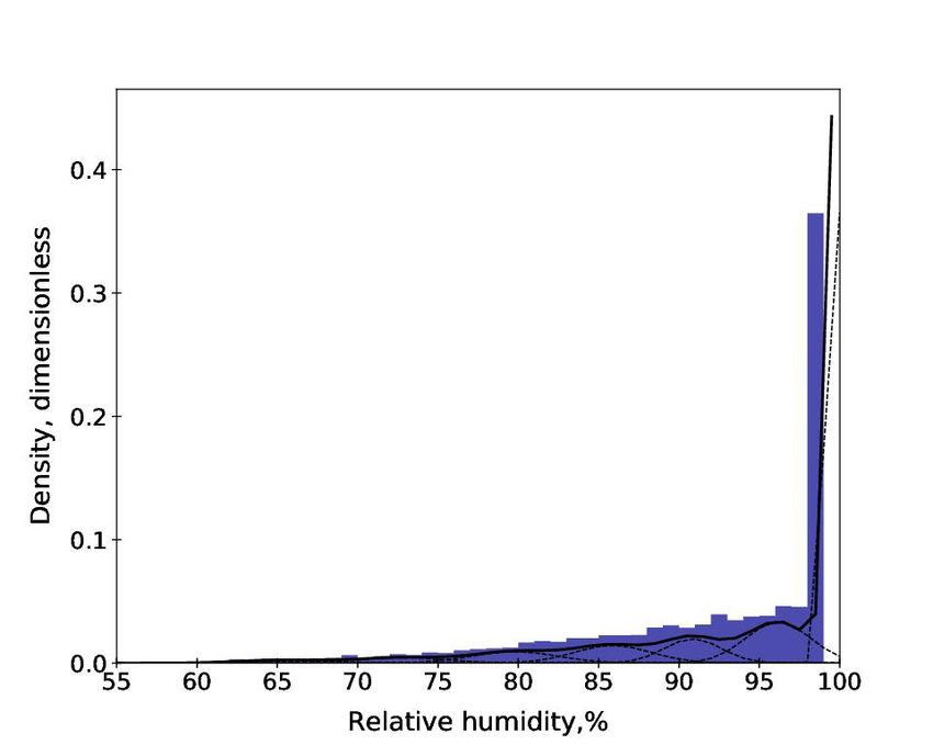
Tecnología en marcha, Edición especial 2020
12         6th Latin America High Performance Computing Conference (CARLA)

     [3]   Corrosion of Metals and Alloys - Corrosivity of Atmospheres - Classification, ISO Standard 9223, 2012.
     [4]   D. Singh, S. Yadav, and J. Saha, “Role of climatic conditions on corrosion characteristics of structural steels,”
           Corrosion Science, vol. 50, pp. 93-110, 2008.
     [5]   J. Solano, and R. Villalobos, Regiones y Subregiones Climáticas de Costa Rica. San José: Instituto
           Meteorológico Nacional, 2000.
     [6]   A. Gómez, “Modelos de mixturas finitas para la caracterización y mejora de las redes de monitorización de la
           calidad del aire,” Master’s Thesis, Statistics and Operative Investigation Department, University of Granada,
           Granada, 2014.
     [7]   Gaussian mixture models, Scikit-learn Project. [Online]. Available in: https://scikit-learn.org/stable/modules/
           mixture.html
     [8]   Statistical functions (scipy.stats), SciPy Project. [Online]. Available in: https:// docs.scipy.org/doc/scipy/referen-
           ce/generated/scipy.stats.norm.html#scipy.stats.norm
You can also read