Gaia Data Release 3: External calibration of BP/RP low-resolution
←
→
Page content transcription
If your browser does not render page correctly, please read the page content below

Astronomy & Astrophysics manuscript no. 43880final                                                                                    ©ESO 2022
                                               June 14, 2022

                                                Gaia Data Release 3: External calibration of BP/RP low-resolution
                                                                      spectroscopic data
                                                  P. Montegriffo 1,? , F. De Angeli 2 , R. Andrae 3 , M. Riello 2 , E. Pancino 4, 5 , N. Sanna 4 , M. Bellazzini 1 ,
                                                     D. W. Evans 2 , J. M. Carrasco 6 , R. Sordo 7 , G. Busso 2 , C. Cacciari 1 , C. Jordi 6 , F. van Leeuwen2 ,
                                               A. Vallenari 7 , G. Altavilla 8, 5 , M. A. Barstow 9 , A. G. A. Brown 10 , P. W. Burgess2 , M. Castellani 8 , S. Cowell2 ,
                                                 M. Davidson11 , F. De Luise 12 , L. Delchambre 13 , C. Diener2 , C. Fabricius 6 , Y. Frémat 14 , M. Fouesneau 3 ,
                                               G. Gilmore 2 , G. Giuffrida8 , N. C. Hambly 11 , D. L. Harrison 2, 15 , S. Hidalgo 16 , S. T. Hodgkin 2 , G. Holland2 ,
                                                 S. Marinoni 8, 5 , P. J. Osborne2 , C. Pagani 9 , L. Palaversa 17, 2 , A. M. Piersimoni 12 , L. Pulone 8 , S. Ragaini1 ,
                                                 M. Rainer 4 , P. J. Richards18 , N. Rowell 11 , D. Ruz-Mieres 2 , L.M. Sarro 19 , N. A. Walton 2 , and A. Yoldas2
arXiv:2206.06205v1 [astro-ph.IM] 13 Jun 2022

                                                      1
                                                          INAF – Osservatorio di Astrofisica e Scienza dello Spazio di Bologna, Via Gobetti 93/3, 40129 Bologna, Italy
                                                      2
                                                          Institute of Astronomy, University of Cambridge, Madingley Road, Cambridge CB3 0HA, UK
                                                      3
                                                          Max-Planck-Institute for Astronomy, Königstuhl 17, 69117 Heidelberg, Germany
                                                      4
                                                          INAF – Osservatorio Astrofisico di Arcetri, Largo E. Fermi, 5, 50125 Firenze, Italy
                                                      5
                                                          Space Science Data Center - ASI, Via del Politecnico SNC, 00133 Roma, Italy
                                                      6
                                                          Institut de Ciències del Cosmos (ICC), Universitat de Barcelona (IEEC-UB), c/ Martí i Franquès, 1, 08028 Barcelona, Spain
                                                      7
                                                          INAF - Osservatorio Astronomico di Padova, Vicolo Osservatorio 5, 35122 Padova, Italy
                                                      8
                                                          INAF – Osservatorio Astronomico di Roma, via Frascati 33, 00078 Monte Porzio Catone (Roma), Italy
                                                      9
                                                          School of Physics & Astronomy, University of Leicester, Leicester LE9 1UP, UK
                                                     10
                                                          Leiden Observatory, Leiden University, Niels Bohrweg 2, 2333 CA Leiden, The Netherlands
                                                     11
                                                          Institute for Astronomy, School of Physics and Astronomy, University of Edinburgh, Royal Observatory, Blackford Hill, Edin-
                                                          burgh, EH9 3HJ, UK
                                                     12
                                                          INAF - Osservatorio Astronomico d’Abruzzo, Via Mentore Maggini, 64100 Teramo, Italy
                                                     13
                                                          Institut d’Astrophysique et de Géophysique, Université de Liège, 19c, Allée du 6 Août, 4000, Liège, Belgium
                                                     14
                                                          Royal Observatory of Belgium, 3 avenue circulaire, 1180, Brussels, Belgium
                                                     15
                                                          Kavli Institute for Cosmology, Institute of Astronomy, Madingley Road, Cambridge, CB3 0HA, UK
                                                     16
                                                          IAC - Instituto de Astrofisica de Canarias, Via Láctea s/n, 38200 La Laguna S.C., Tenerife, Spain
                                                     17
                                                          Rud̄er Bošković Institute, Bijenička cesta 54, Zagreb, Croatia
                                                     18
                                                          STFC, Rutherford Appleton Laboratory, Harwell, Didcot, OX11 0QX, United Kingdom
                                                     19
                                                          Department of Artificial Intelligence, Universidad Nacional de Educación a Distancia, c/ Juan del Rosal 16, E-28040 Madrid,
                                                          Spain
                                                     Received April 27, 2022; accepted May 23, 2022

                                                                                                                  ABSTRACT

                                                     Context. Gaia Data Release 3 contains astrometry and photometry results for about 1.8 billion sources based on observations collected
                                                     by the European Space Agency (ESA) Gaia satellite during the first 34 months of its operational phase (the same period covered Gaia
                                                     early Data Release 3; Gaia EDR3). Low-resolution spectra for 220 million sources are one of the important new data products included
                                                     in this release.
                                                     Aims. In this paper, we focus on the external calibration of low-resolution spectroscopic content, describing the input data, algorithms,
                                                     data processing, and the validation of the results. Particular attention is given to the quality of the data and to a number of features
                                                     that users may need to take into account to make the best use of the catalogue.
                                                     Methods. We calibrated an instrument model to relate mean Gaia spectra to the corresponding spectral energy distributions (SEDs)
                                                     using an extended set of calibrators: this includes modelling of the instrument dispersion relation, transmission, and line spread
                                                     functions. Optimisation of the model is achieved through total least-squares regression, accounting for errors in Gaia and external
                                                     spectra.
                                                     Results. The resulting instrument model can be used for forward modelling of Gaia spectra or for inverse modelling of externally
                                                     calibrated spectra in absolute flux units.
                                                     Conclusions. The absolute calibration derived in this paper provides an essential ingredient for users of BP/RP spectra. It allows users
                                                     to connect BP/RP spectra to absolute fluxes and physical wavelengths.
                                                     Key words. catalogues – surveys – instrumentation: photometers; spectrographs – techniques: photometric; spectroscopy

                                                                                                                           1. Introduction
                                                 ?                                                                         The European Space Agency (ESA) mission Gaia (Gaia Col-
                                                   Corresponding author: P. Montegriffo
                                               e-mail: paolo.montegriffo@inaf.it                                           laboration et al. 2016a) is designed to be self-calibrating for the
                                                                                                                                                                      Article number, page 1 of 33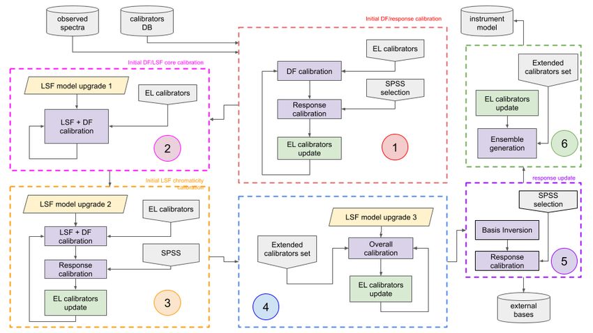
A&A proofs: manuscript no. 43880final

large majority of its data products. For example, the core product      IM presented here to allow for the simulation of Gaia-like mean
of the mission, namely exquisitely accurate and precise astrome-        spectra from a given spectral energy distribution (SED); for ex-
try for ' 1.8 billion celestial sources, is entirely based on obser-    ample a synthetic stellar spectrum or an absolute-flux-calibrated
vations obtained by the mission itself (relative positions at differ-   measured spectrum.
ent epochs and the relative colours of the sources), while external         In this paper, we illustrate how the BP/RP IM is derived
data are only used for validation (Lindegren et al. 2021). Analo-       and how internally calibrated mean BP and RP spectra are con-
gously, the removal of any instrumental imprint and/or space- or        verted into ECS, discussing the performances and the limitations
time-dependent inhomogeneities from the mission all-sky pho-            of the final products. After giving an overview of the external
tometry and spectrophotometry is achieved using repeated mea-           calibration approach (Sect. 2) and a description of the external
surements of large sets of internal calibrators (Riello et al. 2021;    calibrators (Sect. 3), we describe the implementation of the IM
Carrasco et al. 2021; De Angeli, F. et al. 2022).                       (Sect. 4) and the method implemented to reconstruct the ECS
     However, within the production chain of photometry and             (Sect. 5). Section 6 is dedicated to the description of the pro-
spectrophotometry, there are two remarkable exceptions to this          cessing scheme and the main results are shown in Sect. 7, while
generally adopted approach:                                             Sect. 8 is dedicated to the validation of the calibrations. Finally,
     1) The physical flux scale, the main ingredient in the con-        in Sect. 9 we discuss a few known problems.
version of internally calibrated fluxes (expressed in e− s−1 ) into
physical units (W m−2 nm−1 ), which is determined using an ex-
ternal set of spectrophotometric standard stars, the Gaia spec-         2. Overview of the problem
trophotometric standard stars (SPSSs; Pancino et al. 2021).             The instrument model (described in detail in Sect. 4) allows us
     2) The physical wavelength scale, required to convert inter-       to relate a mean BP or RP spectrum to the corresponding SED
nal pseudo-wavelength labels (pixels; see Sect. 2) associated to        via an integral equation of the following kind:
fluxes in BP and RP spectra into wavelengths in physical units
(nm), achieved (mainly) thanks to a set of external spectra of                   Z
sources with strong emission lines at known wavelength.                 ne (u) =    I(u, λ) · n p (λ) dλ,                           (1)
     As there is no way to infer these scales from Gaia data alone,
it is necessary to make use of external calibration data.               where the observed spectrum ne (u) is the internally calibrated
     The BP and RP Instrument Models (IMs), which include               mean spectrum in units of e− s−1 (u denotes a coordinate in data
these two fundamental components, depend on a number of fac-            space, often referred to as a pseudo-wavelength) and the kernel
tors (the dispersion relation, the instrument response, and the line    I is a combination of few components:
spread function (LSF); see Sects. 2 and 4), which are derived us-            (i) the LSF, that is, the instantaneous one-dimensional in-
ing external data in the process known as absolute calibration.         tensity distribution in the spectrum of a monochromatic point
The IM is the fundamental tool for forward modelling of BP              source;
and RP observations, starting from a theoretical model spectrum,             (ii) the dispersion model, that is, the relation that links abso-
with the main goal being to facilitate the inference of astrophys-      lute wavelengths to pseudo-wavelength coordinates; and
ical parameters from their BP/RP spectra by comparison on the                (iii) the response model, which represents the ratio between
plane of observations (Creevey, O., L et al. 2022). Once the pa-        the number of detected photons for wavelength interval and the
rameters of the IM have been estimated (see Sect. 6), the model         number of photons per wavelength interval entering the tele-
can also be used in the opposite direction, that is, to transform       scope aperture.
an internally calibrated mean BP/RP spectrum (De Angeli, F. et               As the detectors are photon-counting devices, all the rela-
al. 2022) into a wavelength- and flux-calibrated spectrum that          tions are expressed in terms of n p (λ), the spectral photon flux
we call an externally calibrated spectrum (ECS). As the IM also         distribution (SPD). The SPD (hereafter expressed in units of
includes the modelling of the LSF at any wavelength, its appli-         photon m−2 s−1 nm−1 ) is related to the source SED via the equa-
cation significantly reduces the effect of photon mixing inherent       tion
to the slit-less spectra produced by the BP and RP spectropho-
tometers, enhancing the effective spectral resolution of ECS. It is                 10−8 λ
important to realise that the IM solves for all the relevant factors    n p (λ) =          f (λ),                                         (2)
                                                                                     hc
(e.g. calibrations of flux and wavelength, and LSF) simultane-
ously, as they are deeply and inseparably entangled in BP/RP            where hc is the product of the Planck constant and the vac-
spectra.                                                                uum speed of light, and the SED f (λ) is expressed in units of
     While BP and RP spectrophotometry has already been used            W m−2 nm−1 (the factor 10−8 compensates for per-nanometre flux
for internal processing in previous releases (Riello et al. 2021),      units; all other measurements and constants are expressed in S.I.
with Gaia Data Release 3 (Gaia DR3, Gaia Collaboration &                units).
et al. 2022) the BP/RP spectra of about 220 million sources are
released for the first time. These can be retrieved from the Gaia           The external calibration concept is based on two key assump-
Archive1 as internally calibrated mean spectra in a continuous          tions: the first is that all differential effects that impact raw ob-
representation (see De Angeli, F. et al. (2022) for details) while      servations (spatial variations of the instrument across the focal
for a subset of sources with G < 15 they will also be provided          plane, different observing configurations, time evolution of in-
as ECS sampled on a standard wavelength grid (see Sect. B for           strument characteristics, etc.) have been removed by the internal
more details on data formats). The Python package GaiaXPy (De           calibration chain (De Angeli, F. et al. 2022) that precedes the ex-
Angeli et al. 2022) has been developed to help users to convert         ternal calibration; the second is that the common reference sys-
spectra from continuous to sampled representation in the inter-         tem defined by the internal calibration is similar to the physical
nal or absolute flux scale (ECS). The tool also implements the          instrument in some unspecified point of the focal plane.
                                                                            These assumptions underlie the design of the external cali-
1
    https://gea.esac.esa.int/archive/                                   bration strategy:
Article number, page 2 of 33
P. Montegriffo et al.: Gaia Data Release 3: External calibration of BP/RP low-resolution spectroscopic data
a) The external calibration model is unique for all sources
and in particular does not depend on source luminosity or colour.
The first assumption above, although plausible, cannot be a pri-
ori guaranteed and any infringement of it will manifest as sys-
tematic differences within different classes of sources.
b) Also, the IM can be parametrised in terms of corrections
to the nominal instrument, which is defined by our pre-launch
knowledge and laboratory measurements made on the satellite
components.
This second point helps to cope with degeneracies that are
present in possible IM solutions: in principle the optimisa-
tion of the IM parameters could be derived from an arbitrarily
large number and variety of standard stars (sources with known
SED from independent ground- or space-based observations) by
matching the predictions of the model with the corresponding
observed BP/RP mean spectra. As discussed by Weiler et al.
Fig. 1. Colour–magnitude diagrams for the whole set of calibrators used
(2020), the traditional approach of deriving a simple response in external calibration processing and validations. On the vertical axes
of the instrument as a function of wavelength —by computing are absolute (left) and apparent (right) G magnitudes.
the ratio between the observed spectrum and the SED for a lim-
ited set of (possibly featureless) calibrators— will not work for a
Gaia-like instrument because of the rather large width of the LSF
compared to the wavelength scale of the response variations. As
a consequence, the derived response changes with the spectral ment components would be constrained by these, allowing for
type of the calibrator: the LSF must be taken into account, creat- degeneracies in the solutions. Implementing the IM as a pertur-
ing the need for a much larger set of calibrators. bation of the nominal model confers the advantage that uncon-
strained components have a reliable a priori estimation. How-
ever, to enforce more observational constraints to the IM, the set
3. Calibrators of primary calibrators has been extended by adding a set of sec-
ondary calibrators, including a wide variety of sources featuring
A reliable calibrator must satisfy several stringent requirements: strong emission lines over the entire wavelength range (mostly
it must be an isolated and point-like source with stable flux and quasi-stellar objects (QSOs) and Wolf Rayet stars). Although
high signal-to-noise ratio (S/N), and it should not be subject to these objects often show variability and require a special treat-
strong interstellar extinction in order to avoid polarisation that ment in the processing (see Sect. 6), they are essential to provide
could cause variations in the measured flux with the observing strong constraints to the wavelength and LSF calibrations. For
geometry and so on (see Pancino et al. 2012; Pancino et al. 2021, the Gaia DR3, a total of 211 peculiar sources have been selected
and references therein). from the literature, including 188 QSOs from the Sloan Digital
The data set of spectrophotometric standard stars (SPSSs)2 , Sky Survey (SDSS; see Lyke et al. 2020, and references therein),
expressly built over the years for the calibration of Gaia pho- 17 young stellar objects (YSOs) from the X-Shooter spectral li-
tometric and spectroscopic data, is composed of 111 stellar brary (Verro et al. 2021), and six emission line sources (ELSs)
sources, calibrated to the CALSPEC3 scale (Bohlin et al. 2014, from STELIB (Le Borgne et al. 2003). Most of these objects
2020) with flux accuracy of about 1% (Pancino et al. 2012; Al- have SEDs only partially covering the Gaia wavelength range:
tavilla et al. 2015; Pancino et al. 2021; Altavilla et al. 2021). this limitation had consequences on the processing strategy, as
The SPSSs have been monitored for short-term constancy at the described in Sect. 6. Finally, we also used the catalogue of the
0.005 mag level over a few hours (Marinoni et al. 2016). The Next Generation Spectral Library (NGSL, Heap & Lindler 2016)
current SPSS release is based on about 25% of the spectra col- for validation purposes, which consists of 348 bright sources
lected for the project; a more complete release, which will con- with magnitude ranging from G = 1.97 and G = 12.0. Figure 1
tain about 200 SPSSs, will be used to calibrate future Gaia re- shows the whole pool of calibrators and validation sources in a
leases. The SPSS data set was recently complemented (Pancino colour–magnitude diagram either in terms of absolute (left) or
et al. 2021) by a second set of 60 stars with looser requirements apparent (right) G magnitudes as function of GBP − GRP colour.
on the absolute accuracy (up to 5%) and flux stability (up to vari-
ations of about 0.05 mag) but including stellar types not con-
tained in the SPSS set (bright O, B and late M stars), the pass- 4. Instrument model
band validation library (PVL). These were originally intended
to be used for validation purposes only, but a subset of these The Gaia satellite observes the sky spinning around its axis
were eventually included in some phases of the actual calibra- (Gaia Collaboration et al. 2016a): the light collected by its tele-
tion of the IM. The consequence of the severe criteria applied scopes is projected onto the focal plane where an array of charge-
to the selection of primary calibrators is that the resulting stellar coupled device (CCD) detectors make measurements while op-
spectra are not independent from a mathematical point of view: erating in time-delay integration (TDI) mode. In the case of Gaia
their principal components span only a subspace of all possible spectrophotometers, two slit-less prisms disperse the light onto
spectral shapes and consequently not all the necessary instru- two separate rows of seven CCDs each, both covering the focal
plane in the across scan (AC) direction. The dispersion direction,
2
http://gaiaextra.ssdc.asi.it:8080/ referred as along scan (AL) being aligned with the transit direc-
3
https://www.stsci.edu/hst/instrumentation/ tion of the projected light, is perpendicular to the AC direction.
reference-data-for-calibration-and-tools/ Each spectrophotometer covers part of the spectral wavelength
astronomical-catalogs/calspec interval, and the two ranges partially overlap: the blue photome-
Article number, page 3 of 33A&A proofs: manuscript no. 43880final
ter (BP) covers the nominal range [330, 680] nm while the red
photometer (RP) covers the range [640, 1050] nm. For each ob-
served source, to limit the telemetry of the satellite, only a small
window around the position of the source is actually read and
transmitted to Earth during each transit. Windows are 60 × 12
pixels wide in each of the AL and AC directions. The maximum
exposure time of an observation (∼ 4.4 s) is fixed by the veloc-
ity by which the image transits on a CCD, but, to avoid satura-
tion, it can be reduced according to the magnitude of the source
by limiting the activation of the reading window to only a por-
tion of the CCD with gates (De Angeli, F. et al. 2022). Sources
brighter than G ' 11.5 are transmitted as 2D windows (called
window class 0, WC0) while for fainter sources, data are binned Fig. 2. Pre-launch nominal dispersion relations for BP and RP instru-
in the AC direction producing 1D spectra of 60 samples (WC1). ments. Different curves refer to all FoV/CCD row combinations.
Each source is observed several times during the lifetime of the
mission under many different observing configurations and con-
ditions (see Carrasco et al. 2021, for an exhaustive description). provided for the centre of each CCD (the dispersion varies in the
The internal calibration (De Angeli, F. et al. 2022) has the com- AC direction) in the form of the coefficients Ai of the expansion
plex task of calibrating all these configurations to reduce spectra
X
AL(ω) − AL(ωre f ) = Ai ωi , (5)
to a common reference system, the mean instrument.
i
If we assume that the dispersion of the prism is perfectly
aligned with the AL direction, then we can model the dispersed where
image of a point-like source in the data space as
– AL(ω) denotes the AL image position in mm,
Z∞ – ω = 1/λ in nm−1 denotes the wavenumber, and
– ωre f = 1/440 nm−1 for BP and 1/800 nm−1 for RP, corre-
=(u, w) = Pτ n p (λ) Pλ (u − ud (λ), w) R(λ) dλ, (3)
sponding roughly to the central wavelength of each instru-
0 ment.
where u is the continuous coordinate in data space in the AL The AL position in pixel units u is obtained by dividing Eq. 5
direction, w is the continuous coordinate in data space in the by the pixel size of a CCD in the AL direction PAL . Nominal
AC direction, Pτ is the telescope pupil area, n p (λ) is the SPD dispersion curves for all FoV/CCD row combinations are shown
of the source, ud (λ) is the dispersion function, Pλ (u, w) is the in Fig. 2. The dispersion curve varies across the focal plane due
effective monochromatic point spread function (PSF) at wave- to the tilt of the prisms with respect to the focal plane assembly:
length λ, and R(λ) is the overall instrument response function. the comparison of the dispersion functions for different AC posi-
This relation assumes indirectly that non-linear effects, such as tions shows that the functions are related through a linear scaling
those produced by charge transfer inefficiency (CTI) effects4 , are to a high degree and are virtually independent from the FoV. We
not important and can be neglected. As all internally calibrated can therefore arbitrarily assume the coefficients for any of the
spectra are binned to 1D windows, we can integrate the previ- CCD rows or FoV and model the generic dispersion function as:
ous equation in the AC direction, obtaining the following model,
which is suitable for describing a mean spectrum: k
N u −1 N
X 1 X 1
ud (λ) = Ai i ,
Z∞ dk · (6)
PAL i=0 λ
ne (u) = Pτ n p (λ) Lλ (u − ud (λ)) R(λ) dλ, (4) k=0
0 where ud (λ) denotes the AL image position in pixel units, coeffi-
cients Ai are arbitrarily assumed as those of CCD row 4, and FoV
where ne is given in units of e− s−1 and Lλ (u) is the effective 1 and dk are the IM parameters to be optimised in the calibra-
monochromatic LSF at wavelength λ obtained by integrating Pλ tion process. For Gaia DR3, we assume a number of parameters
in the AC direction. This is the explicit form of Eq. 1. A detailed Nu = 3. Lower order parameters can be interpreted as follows:
description of each factor of the model is given in the following parameter d0 represents the zero point of the dispersion relation
subsections. and by construction is the reference AL position ure f correspond-
ing to the reference wavenumber ωre f ; and parameter d1 is the
4.1. Dispersion model scale of the dispersion relation. The nominal values are d0 = 30,
d1 = 1.0, and d2 = 0.0 for both BP and RP instruments.
Airbus Defence and Space (DS), the company in charge of de-
veloping and building the Gaia satellite, provided nominal dis-
persion functions based on chief-ray analysis for the BP and RP 4.2. The line spread function model
prisms in units of millimetres as a function of wavelength, by fit- The LSF model is the only component of the IM that cannot
ting a sixth-degree polynomial to the unperturbed Gaia optical be implemented as a simple perturbation of a nominal model,
design. For each field of view (FoV), dispersion functions are as in the cases of the dispersion and response models. Numeri-
4
CTI, by delaying the release of the charge by a physical pixel as CCD cal monochromatic LSFs were provided by Airbus DS for test-
charges scroll in the AL direction, would result in a deformation of the ing purposes for each combination of FoV and CCD row; Fig. 3
source spectrum that depends not only on the source SED but also on the shows two sets of these LSFs computed at wavelength λ = 440
scene of the observation, i.e. the temporal sequence of sources observed nm for the BP instrument (left) and λ = 800 nm for the RP in-
by that particular pixel immediately before the considered transit. strument (right). These models were built upon the optical PSF
Article number, page 4 of 33P. Montegriffo et al.: Gaia Data Release 3: External calibration of BP/RP low-resolution spectroscopic data
Fig. 3. Example of pre-launch nominal monochromatic LSF computed
at wavelength λ = 440 nm (left) and λ = 800 nm (right). Different
curves represent the LSF for each FoV/CCD row combination.
model of the telescope, which included optical aberrations based
on laboratory measurements of the wavefront error (WFE) maps
made on the telescope mirrors. The great variations in the shapes
of the LSF shown in the figure are essentially due to variations in
the WFE map from one FoV/CCD pair to the other. The problem
is that these WFE maps are not applicable to the flying instru- Fig. 4. LSF basis functions. Left: First four basis functions of matrix U
ment because several factors (changes in physical conditions, as a function of the AL coordinate. Right: First four basis functions of
matrix W as a function of wavelength.
mechanical stress of the launch, defocusing of the instrument,
etc.) lead to them changing in an unpredictable way.
The strategy adopted for the current model implementation,
which is explained in more detail in Appendix C, is to create a
large sample of theoretical PSFs based on the optical design of where L(u, λ) is the numerical mean LSF of the theoretical set
Gaia, including randomly generated realistic WFE maps: these and dm,n are the IM parameters that are fitted during the ex-
optical PSFs are then converted to effective PSFs that include ternal calibration processing. As explained in Appendix C, the
a number of effects (charge diffusion, smearing introduced by LSF wavelength modelling requires roughly half the dimensions
TDI, pixel integration) to account for the discretised nature of needed for AL dependency modelling, hence `1 ' 2`2 . Reiter-
the data. Effective PSFs are then marginalised in the AC di- ating the caveat expressed at the beginning of this section re-
rection to obtain a set of numerical LSFs sampled on a two- garding the absence of a proper nominal LSF model, when all
dimensional grid in spatial and wavelength coordinates. These parameters dm,n are set to zero the LSF coincides with the mean
numerical LSFs are then used to build a set of two-dimensional
basis functions to allow the LSF to be modelled with a minimum numerical model L(u, λ).
number of free parameters for a given accuracy. The reduction to Equation 7 represents an undispersed LSF centred on the ori-
the 2D basis functions is achieved by means of generalised prin- gin of the U bases. The dispersed LSF in the data space can be
cipal component analysis (GPCA, Ye et al. 2004), a fast and ef- obtained by shifting the origin by an amount given by the dis-
ficient algorithm for 2D image compression used to concentrate persion relation as seen in Eq. 4: L (u − ud (λ), λ). However, it
relevant information of a given data set in a small number of di- is worth noting that the LSF origin does not necessarily coin-
mensions. Unlike the usual principal component analysis, GPCA cide with its centroid: the centroid is an intrinsic property of the
is able to preserve the spatial locality of pixels in an image by LSF, and in the case of a symmetric LSF is naturally given by the
projecting the images to a vector space that is the tensor product point of symmetry ξ, that is L(ξ − u) = L(ξ + u) ∀u, but in general
of two lower dimensional vector spaces. These two vector spaces the LSF is not symmetric and its shape can change with wave-
are designed by matrices U and W whose columns represent the length, introducing some degeneracy between the chromaticity
basis functions with which the dependencies are modelled along and the dispersion. As sketched in Fig. 5, the dispersion model
the spatial coordinate u and the wavelength coordinate λ, respec- of Eq. 6 provides the location of the LSF origin: as far as the
tively. Figure 4 shows the first four bases for vector space U instrument model is concerned, the degeneracy between disper-
(left) and W (right). The U and W bases are interpolated to con- sion and chromaticity has little significance because the disper-
tinuous variables (u, λ) by 1D interpolation. To ensure that the sion model and the LSF origin are consistently defined; however,
interpolation for the U bases satisfies the ‘shift invariant sum’ physical interpretation of the data requires a dispersion relation
condition, which preserves the underlying function normalisa- that gives the centroid of the monochromatic LSF as a function
tion independently from the subpixel position of the sampling of wavelength. This dispersion relation is provided as a lookup
grid, these bases were then fitted with an S-spline model (Linde- table where the centroid u0 is computed at each wavelength λ by
gren 2009). The interpolation for W bases is achieved by a cubic solving the non-linear equation:
spline. The model for the LSF is finally given by
`1 X
`2
Z∞
L(u0 + u, λ) w(u/s) du = 0,
X
L(u, λ) = L(u, λ) + dm,n · Um (u) · Wn (λ), (7) (8)
m=1 n=1 −∞
Article number, page 5 of 33A&A proofs: manuscript no. 43880final
Fig. 5. Definition of centroid, origin, and location. Top: A schematic
monochromatic LSF at a given wavelength λ0 with origin u = 0 and
centroid u = u0 . Bottom: Location κ of the LSF in the data stream of
sample values: a narrow emission line at wavelength λ0 is overlying a
continuous signal at k = κ. Fig. 6. Pre-launch nominal responses for BP and RP instruments.
where the weighting function w is the Tukey’s bi-weight: These quantities were initially measured by Airbus DS during
on-ground laboratory test campaigns and are plotted in Fig. 6.
2 As can be seen, the steepest features of these curves are the BP
z 1−z
2
if |z| < 1
and RP cut-offs produced by the prism transmittance curves, and
w(z) =
(9) the steep BP drop around ' 400 nm which is mainly due to mir-
0 otherwise,
ror reflectivity. Laboratory measurements showed that the pre-
cise location, that is, in wavelength, of the cut-off varies across
and the scale parameter s = 2.7 is a value suitable for the Gaia the focal plane due to the uneven thickness of the prism coating
case (Lindegren 2006). This dispersion function is provided for (which is a few nm in both instruments). Moreover, combining
both BP and RP instruments as a single CSV file tabulated for measurements taken all over the focal plane results in a further
wavelengths ranging from 320 nm to 1100 nm in steps of 0.5 smearing of the nominal curve. Therefore, a suitable modelling
nm5 . of the actual response cut-offs has been achieved by assuming
the nominal curves, degrading the wavelength resolution by con-
volution with a rectangular window of width varying with the
4.3. Response model
spectral dispersion per pixel, and re-shaping the cut-off mathe-
The response R(λ) defined in Sect. 2, as the ratio between the matically with a two-parameter Gauss error function for RP and
number of detected photons and the number of photons entering a two-parameter complementary error function for BP to control
the telescope aperture per wavelength interval, is modelled as the wavelength position λC and the slope σC of these features
the product of the individual responses of each physical element (the tabulated transmittance curve is in practice truncated just
(e.g. primary mirror, secondary mirrors) hit along the optical before the cut-off and multiplied by the error function to mimic
path. It changes across the focal plane, and depends on the ob- the cut-off shape). Nominal values for (λC , σC ) are (667.9, 4.71)
serving configuration of each source and transit (gates, window and (631.0, 4.0) for BP and RP, respectively. The corresponding
class) and on time (contamination and decontamination issues). curves are represented in Fig. 6 as blue (BP) and red (RP) thick
Assuming that all these dependencies have been accounted for lines. It is well known that the actual on-board overall response
by the internal calibration, we are left with a function of the was heavily affected by rapid and discontinuous variations due
wavelength alone. to water vapour contamination of the satellite instrument com-
The nominal pre-launch response curve for the mean BP and ponents (Gaia Collaboration et al. 2016b) and to the various de-
RP instruments can be described (Jordi et al. 2006) as the prod- contamination campaigns. The internal calibration initialises the
uct of the following elements: internal reference system using only high-quality data collected
in periods of low and slowly varying contamination (De Angeli,
RN (λ) = T 0 (λ)ρatt (λ)Q(λ)T p (λ), (10) F. et al. 2022), which ensures that the mean instrument response
is not too different from the nominal R∗N (λ; λC , σC ). Neverthe-
where less, to be able to model any deviation from the nominal curve,
the response is multiplied by a parametric function:
– T 0 (λ) is the telescope (mirrors) reflectivity;
– ρatt (λ) is the attenuation due to rugosity (small-scale varia- R(λ) = R∗N (λ; λC , σC ) · Rd (λ; ri ). (11)
tions in smoothness of the surface) and molecular contami-
nation of the mirrors; Parameters ri are referred to as response shape parameters to
– Q(λ) is the typical CCD quantum efficiency curve; distinguish them from the two response cut-off parameters λC
– T p (λ) is the prism (fused silica) transmittance curve includ- and σC ; their nominal values are all zeros. The distortion model
ing the filter coating. Rd is implemented as the exponential of a linear combination of
a set of basis functions R in the AL sampling space u:
5
Available at https://www.cosmos.esa.int/web/gaia/
Rd (u) = e ,
P
ri Ri (u)
dr3-bprp-instrument-model (12)
Article number, page 6 of 33P. Montegriffo et al.: Gaia Data Release 3: External calibration of BP/RP low-resolution spectroscopic data
which is transformed to wavelength space λ through the disper- functions whose images through the dispersed LSF model are the
sion relation: bases of the internal representation: the great advantage of this
approach with respect to solving Eq. 15 directly is that it requires
du
Rd (λ) = Rd (ud (λ)) . (13) inverting the integral equation for a set of analytic functions that
dλ are by definition noise-free. We refer to these functions φn as the
The exponential form guarantees the non-negativity of the over- inverse bases hereafter.
all model, while modelling in the sample space ensures the nat- To choose the most suitable representation for the inverse
ural instrument spectral resolution, avoiding over-fitting where bases, it is useful to review the representation used for internally
the spectral resolution is lower. The basis functions Ri used for calibrated mean spectra described in Carrasco et al. (2021) and
the Gaia DR3 models are spline functions of second order with De Angeli, F. et al. (2022) and summarised here for convenience.
an initial uniform knot spacing in u that becomes non-uniform The basis functions implemented for Gaia DR3 are orthonormal
in later processing stages (see Sect. 6 for details). The full set of Gauss-Hermite functions ϕn (θ) where a linear transformation is
IM response parameters to be optimised is therefore (ri , λC , σC ): set between the pseudo-wavelengths axis u and the argument of
when they are set to their nominal values, the response model the Hermite functions θ as:
closely resembles the nominal model. u − ∆θ
θ= . (19)
Θ
5. Basis inversion and SED reconstruction The number of bases for Gaia DR3 has been set to N = 55 for
both BP and RP spectra. An optimisation post-process is applied
Once the instrument model is defined, Eq. 4 can be used to esti- to mean spectra basis functions to concentrate most of the infor-
mate the spectral photon flux distribution n p (λ) corresponding to mation in the lower order spectral coefficients: this optimisation
an observed spectrum ne (u). Obtaining the SPD/SED allows the takes the form of a rotation of the bases specified by a square ma-
user to inspect Gaia spectra in a format that is more intuitive and trix VC . This rotation has no consequence for the basis inversion
of common usage. It may be convenient to define an effective algorithm described here because, whenever Eq. 18 is satisfied,
spectral photon distribution as: the inverse bases for the optimised bases are simply obtained by
n∗p (λ) = n p (λ) · R(λ), (14) applying the same rotation matrix to the inverse basis set φn . The
model chosen to represent each φn function is a linear combina-
so that tion of the same bases that model their image through the instru-
ment model, that is, a linear combination of Hermite functions:
Z∞
ne (u) = Pτ n∗p (λ) Lλ (u − ud (λ)) dλ. (15) K
X
0 φn (θ) = hk,n · ϕk (θ), (20)
k=1
The effective spectrum is the observed spectrum deconvolved
by the LSF function and transformed to the wavelength space with the same mapping between axes u and θ as adopted for the
through the dispersion relation (and scaled by some factor). bases used to represent internally calibrated spectra:
Therefore, its shape will preserve the basic features of the ob-
Z∞ XK
served spectrum. However, Eq. 15 is a Fredholm integral equa- u − ∆θ ud (λ) − ∆θ
! !
tion of the first kind, which is difficult to solve for the un- ϕn = Pτ hk,n ϕk Lλ (u − ud (λ)) dλ.
Θ Θ
known n∗p (λ) because such integral equations are often ill-posed k=1
0
problems: large variations in the solution n∗p (λ) can occur for a (21)
slightly perturbed observable ne (u) (as is the case here, as ne is
affected by noise). However, as BP/RP mean spectra are mod- The reason for choosing such a model is that, as in the case of
elled as a linear combination of basis functions (Carrasco et al. the effective photon distribution, left and right bases should share
2021): the same basic features, as the function on the left hand side of
X the equation is a smeared version of that on the right hand side
ne (u) = bn ϕn (u), (16) once mapped to the same axis u.
n We could solve Eq. 21 for coefficients hk,n in a least-squares
sense by sampling ϕn on a sufficiently dense and extended grid
an interesting solution can be found by modelling the effective on the θ axis, but in this case the optimal number of bases K of
spectral photon distribution as a linear combination of the same the model would be undefined and it would not be clear whether
spectral coefficients bn with a particular set of bases: or not a limit to this number were set by some hidden condi-
N tion. A more appealing possibility is to project Eq. 21 into the
coefficient space bn of mean spectra, where the nth function ϕn is
X
n∗p (λ) = bn φn (λ), (17)
n=1
represented by definition by a vector of coefficients that are all
null except the nth one equal to unity. In matrix notation, let b
where the φn bases satisfy the following condition: denote the array of coefficients, s a mean spectrum sampled on a
given grid u of U points, and D ∈ RU×N the design matrix whose
Z∞ element Dnu is the value of the nth Hermite function evaluated at
ϕn (u) = Pτ φn (λ) Lλ (u − ud (λ)) dλ. (18) the uth pixel grid point. Consequently,
0
s = D · b, (22)
In practice, the externally calibrated spectral photon distribution and
(and related SED) corresponding to each pair of observed BP
and RP spectra can be reconstructed by finding a set of proper b = D† · s, (23)
Article number, page 7 of 33A&A proofs: manuscript no. 43880final
where D† ∈ RN×U is the pseudo-inverse of the design matrix (see where R(λ) is the instrument response and hc the product of the
Appendix D for details). The integrals of Eq. 21 can be com- Planck constant and the vacuum speed of light, then we get
puted numerically by trapezoidal integration over a fine regular
wavelength grid with Λ points and step δλ extending over the np = DϕP · H · VCT · b, (33)
wavelength interval where the response is not null: let L ∈ RU×Λ
represent the instrument dispersed LSF model kernel sampled which is the SPD in units of photons s−1 m−2 nm−1 , and
over that discrete grid, with the (i, j)th element being
fλ = DϕE · H · VCT · b, (34)
Li, j = Pτ · Lλ j ui − ud (λ j ) δλ. (24)
which is the SED in units of Wm−2 nm−1 .
We can write an equation like Eq. 21 for each of the left N Her- As the design matrices of Eqs. 31-32 depend on the inverse
mite basis functions: if the left term is interpreted as a column of of the instrument response function, the sampling wavelength
the design matrix D, then all the N relations can be condensed grid must be limited to the range [330, 650] nm for BP and
into one single equation: [635, 1050] nm for RP in order to avoid large errors in the re-
constructed spectra.
D = L · Dϕ · H, (25) The BP and RP instruments produce two partially overlap-
ping SPDs and SEDs: these are combined into a single distribu-
where Dϕ ∈ RΛ×K is the design matrix for the right ϕk bases sam- tion by computing a weighted mean in the overlapping region
pled on the wavelength integration grid, while matrix H ∈ RK×N [λlo , λhi ], where the weight varies linearly with wavelength:
contains in its columns the set of coefficients hk,n that define the
shape of each inverse basis. By multiplying Eq. 25 by D† from λ − λlo
wBP (λ) = 1 − , (35)
the left we finally obtain: λhi − λlo
IN = D† · L · Dϕ · H, (26) and
where the left hand term is the (N ×N) identity matrix. By setting wRP (λ) = 1 − wBP (λ), (36)
for λlo < λ < λhi .
B = D† · L · Dφ , (27) BP and RP spectra coefficients are accompanied by the co-
variance matrix Kbb : this is used to calculate the covariance ma-
it is evident that the problem can be solved if B is a square matrix trix for the sampled spectrum, which in the case of the SED is
with K = N, that is, the number of inverse bases is equal to the computed as
number of bases for mean spectra representation. In this case, T
the matrix H that defines the basis functions for the externally Kff = DϕE · H · VCT · Kbb · DϕE · H · VCT . (37)
calibrated spectra is simply given by:
The square roots of the diagonal elements of Kff are the errors
H = B−1 . (28) associated with the sampled SED.
The model for inverse bases consists of a matrix of coeffi-
cients H for each of the BP and RP instruments. Let λ be the 6. Processing
wavelength grid over which we sample the externally calibrated
spectrum corresponding to a pair of BP and RP observed spec- The instrument model has been designed to reproduce the nom-
tra and Λ be the dimension of vector λ. We can build a design inal instrument model when all parameters are set to their nom-
matrix Dϕ ∈ RΛ×N by sampling the N Hermite functions on the inal values: these parameters are di for the dispersion (Eq. 6),
grid: dm,n for the LSF (Eq. 7), and ri , λC , σC for the response model
(Eqs. 11-12). The concept of nominal refers to the dispersion
ud (λ) − ∆θ function and to the overall response curve, for which pre-launch
θ= . (29)
Θ laboratory measurements are available. The LSF model instead
is initialised as the mean of a large number of theoretical LSF
If VC is the orthogonal rotation matrix that defines the optimi- models: for this reason it corresponds to a flat WFE map and is
sation of the basis functions for the internally calibrated mean symmetric. Model parameter optimisation can be fulfilled with a
spectra, we obtain that the sampled effective spectral photon dis- sufficient number of calibrators by minimising in a least squares
tribution is defined as sense a χ2 -based cost function
n∗p = Dϕ · H · VCT · b. (30) χ2 = rT · W · r, (38)
If we build two more design matrices DP ϕ and DE ϕ whose ele- where the array of residuals r and the weight matrix W can be
ments are respectively defined as evaluated in two different spaces:
1 1. Sample space: the observed BP/RP mean spectrum is sam-
DϕP i, j = Dϕ i, j , (31) pled according to Eq. 22:
R(λi )
and r = D · b − Iu,λ · np , (39)
1 108 hc where Iu,λ represents the instrument matrix sampled on the
DϕE i, j = Dϕ i, j , (32) wavelength array of the source SPD and on the same AL
R(λi ) λi
Article number, page 8 of 33P. Montegriffo et al.: Gaia Data Release 3: External calibration of BP/RP low-resolution spectroscopic data
Fig. 7. Processing scheme.
grid as the mean spectrum; (Iu,λ np ) represents the discretised When optimisation is carried out in sample space, the AL
version of Eq. 1, and the weight matrix is computed as grid used to compare sampled spectra is usually oversampled
−1 by some factor with respect to the Gaia pixel, and therefore
W = D · Kbb · DT + Iu,λ · Kpp · ITu,λ , (40) the coefficients covariance matrix transformed to sample space
(D · Kbb · DT ) (hereafter samples covariance) does not have full
where Kbb is the covariance matrix of the spectra coefficients, rank and cannot generally be inverted. A first obvious solution
the product DKbb DT is the pixel covariance matrix of the is to take into account only the diagonal elements of the samples
sampled BP/RP spectrum, and Kpp represents the covariance covariance, even if the off-diagonal elements are not negligible
matrix of the source SPD. because mean spectra are continuous functions and hence ran-
2. Coefficient space: the model prediction is projected in the dom noise will manifest as random wiggles in the form of long-
coefficient space according to Eq. 23 range correlations between pixels. A formal solution for a cor-
rect weighting scheme in sample space is to compute the weight
r = b − D† · Iu,λ · np , (41) matrix as:
T
and the weight matrix is the inverse of the sum between co- W = D† · Kbb −1 · D† , (43)
efficients and projected SPD covariances: where the pseudo-inverse of the samples covariance matrix D†
T −1 has been defined in Eq. D.4. This approach was tested but some
W = Kbb + D† · Iu,λ · Kpp · D† · Iu,λ . (42) occasional numerical instabilities discouraged us from using it
for the present calibrations. Cost evaluation in coefficient space
In all scenarios, we include the usage of the covariance matri- would solve the problem of the invertibility of the matrix, allow-
ces for both the observed BP/RP spectra and the calibrator SPDs ing for a full exploitation of spectra covariances. However, this
to allow for a total least-squares regression analysis of the data approach could not be followed for the current release because
(Huffel & Vandewalle 1991). Although the SPD covariance ma- of the incomplete wavelength coverage of many emission line
trix would be extremely important to properly account for sys- calibrators used in the optimisation process (Eq. 23 implicitly re-
tematic effects of wavelength calibration errors, especially in re- quires the sampled spectrum to extend over the entire AL range).
gions where the SPD changes steeply with the wavelength for For calibrators with incomplete wavelength coverage, χ2 compu-
certain spectral types, only errors on fluxes are usually avail- tation was limited to the available section of the model spectrum,
able in the literature. Therefore, only BP/RP covariances are excluding a safety margin of a couple of pixels where truncation
full matrices while SPD covariances are simply diagonal matri- occurs because the redistribution of light produced by LSF will
ces populated with the corresponding variances on the sampled cause some systematic difference between the partial spectrum
flux. Moreover, total regression is generally highly demanding and the one that would have been obtained by a complete SPD.
in terms of computational cost because it requires an evaluation For this reason, we decided to carry out the cost evaluation in
and inversion of the covariance matrix at each step of the solver, sample space.
and has therefore only effectively been taken into account in the Provided that the cost function is not linear with respect to
final stages of the calibration, as is clarified below. the model parameters, the optimisation process can be carried
Article number, page 9 of 33A&A proofs: manuscript no. 43880final
out using an implementation of the differential evolution algo-
rithm (DEA) as described by Storn & Price (1997): although
this class of algorithms has been shown to achieve global op-
timisation with a natural ability to escape local minima traps in
the χ2 space, we find it convenient to proceed with the boot-
strapping of the model by limiting the number of free parame-
ters at the first stages of the processing, and gradually enhancing
the model complexity (i.e. increasing the number of parameters)
only when convergence is progressively achieved. This led to a
complex processing scheme that is sketched in Fig. 7.
Calibrators are divided into two groups, absolute flux or
primary calibrators (labelled SPSS) and secondary calibrators,
sources with emission line features (labelled EL calibrators). As
explained in Sect. 3, the latter group contains potentially variable
sources. To overcome this problem, an update process equivalent
to a grey flux calibration is implemented for these calibrators:
the input SPD of each EL source is scaled by a parameter that is
evaluated at each calibration cycle to minimise the squared resid-
uals between the current model prediction and the corresponding
observed mean spectrum. In the first stage of the processing, the
response model is initialised with a low number of shape param-
eters (see Eq. 11, 8 parameters for BP, 5 for RP), while cut-off
parameters are set to their nominal values, the dispersion model Fig. 8. BP and RP response curves traced by the ratio between effective
degree is set to 1, and the LSF model is symmetric. This stage SPD computed from BP and RP spectra and source SPDs from ground-
is designed to provide a reliable initialisation of the dispersion based observations. Top: Data are plotted against wavelength; black tri-
relation and the response shape: the cost evaluation is limited angles mark the position of Balmer lines. Bottom: Residuals between
data and the response models are plotted against pseudo-wavelengths.
to the central region of the spectra, avoiding the wings and the
BP pseudo-wavelengths have been swapped left-to-right, while RP data
cut-off regions; the optimisation of the dispersion parameters, are shifted by 60 samples. Blue- and red-filled triangles mark the posi-
based on the EL calibrators, is alternated with the optimisation tion of BP and RP cut-of,f respectively, while blue and red open trian-
of the response shape, which is achieved by using a selection gles show where the response drops to zero.
of featureless SPSSs. Each optimisation cycle typically consists
of approximately 3000-4000 DEA iterations involving about 50
walkers (different realisations of model parameters, initially dis-
tributed randomly around the starting set of parameters). The it-
erations stop when the individual costs from all the walkers con- in order to sort the displayed data according to wavelength. RP
verge to a common value. The set of parameters with the low- data are offset by 60 samples in pseudo-wavelength to avoid su-
est cost is used to initialise the subsequent optimisation cycle. perposition with BP. It is possible to recognise the signs left in
Once convergence is reached, the second stage begins, which the data by the first Balmer absorption lines (Hα through H )
entails modelling the shape of the central part of the LSF: the as peaks highlighted in the plots. Interestingly, a wavy regular
LSF model is initialised with (`1 , `2 ) = (4, 1) bases, and LSF pattern is visible at all wavelengths with a nearly constant fre-
and dispersion parameters are optimised together to model any quency in the pseudo-wavelength space. The origin of this pat-
possible asymmetry of the LSF core. A second upgrade to the tern is not fully understood; it could be related to wiggles in the
LSF model is made in stage 3 where the number of bases is in- mean spectra (De Angeli, F. et al. 2022). Using this data, we up-
creased to (`1 , `2 ) = (4, 2) to allow modelling of any chromatic- graded the instrument response distortion model by increasing
ity effect: an LSF and dispersion parameter fit is alternated with the number of spline knots to model these wiggles, especially in
response model adjustment and EL source update. In stage 4, the the range [500, 800] nm, carefully excluding the signature left
LSF and dispersion models are set to their final configurations, by the Hα line (the response model must not be a function of any
the number of response shape parameters are doubled while the source astrophysical parameter). The total number of response
cut-off parameters are left free to change; all model parameters parameters is 26 for BP and 23 for RP. The model curves rep-
are optimised together using an extended set of calibrators (EL resented in the top plot were computed after this upgrade. The
+ SPSS). The number of bases is set to (`1 , `2 ) = (7, 3) for BP last stage of the processing is dedicated to the creation of the en-
and is left unchanged for RP; in both instruments the dispersion semble of instrument models: the DEA solver is run on the last
model degree is set to 2. In stage 5, the basis inversion process instrument models until parameter relaxation is achieved (typi-
is performed to allow the reconstruction of the effective SPD for cally after about 400 iterations), and then all the 50 walkers are
the SPSS: these are divided by the corresponding source SPDs saved into the database providing the 50 instrument models. The
to obtain the data shown in Fig. 8. This plot was obtained using walker with the lowest chi-square is chosen to represent the in-
a subset of 41 SPSSs selected to be as featureless as possible strument model, which enables forward modelling to simulate
and, given the definition of effective spectra in Eq. 14, it traces mean BP and RP spectra or inverse modelling to provide SEDs
the overall instrument response curves. The top plot shows data through the inverse basis representation. The ensemble instead
plotted as a function of wavelength. The bottom plot shows the is used to derive the uncertainties in the simulated spectra. The
residuals between data and model represented as function of the instrument model ensemble and the inverse bases are used in the
AL coordinate (or pseudo-wavelength); given that the dispersion GaiaXPy tool (De Angeli et al. 2022) to simulate mean spectra
direction of the BP instrument is inverted with respect to that and to generate sampled Gaia BP and RP calibrated spectra in
of the RP instrument, BP data have been mirrored horizontally the absolute system.
Article number, page 10 of 33P. Montegriffo et al.: Gaia Data Release 3: External calibration of BP/RP low-resolution spectroscopic data
Fig. 9. Visual representation of instrument matrix for BP (left panel) and RP (right panel) instruments. Green dashed curves are the dispersion
relations, and white curves sum up the matrix columns and represent the response curves.
Fig. 10. Three selected columns of the instrument matrix for BP (top Fig. 11. Three selected rows of the instrument matrix for BP (top panel)
panel) and RP (bottom panel) in logarithmic scale. The curves repre- and RP (bottom panel). The curves represent the percentage as function
sent the dispersed monochromatic LSFs at three different wavelengths of wavelength of the incoming photons that are accumulated in the cor-
rescaled by 100 to represent a percentage distribution. responding data sample.
7. Results respectively, (ii) each column represents a monochromatic dis-
persed LSF scaled by the response (the response curve is over-
The final BP and RP instrument models were used to create plotted in white) at that wavelength and the telescope pupil area,
Fig. 9 where the corresponding instrument matrices Iu,λ are rep- and (iii) the loci of LSF maxima, highlighted by the dashed
resented: this plot shows at a glance how BP and RP mean spec- green lines, correspond to the dispersion functions, then we can
tra are simulated for a given SPD. The instrument matrix can be visualise the mean spectrum formation by splitting the incom-
used to express Eq. 1 in a discretised form as already done in ing SPD into packets of photons according to their wavelength.
Eq. 39: a mean spectrum is the row-by-column product of the These are then distributed following the corresponding matrix
instrument matrix with the SPD (sampled on the same wave- column profile, and the final mean spectrum is given by the ac-
length grid of Iu,λ ). Provided that: (i) columns and rows repre- cumulation on the u axis of each dispersed packet. One of the
sent small intervals of wavelengths and AL sample coordinates elements that catches the eye is that the dispersion direction is
Article number, page 11 of 33You can also read