Fast infrared radiative transfer calculations using graphics processing units: JURASSIC-GPU v2.0
←
→
Page content transcription
If your browser does not render page correctly, please read the page content below
Geosci. Model Dev., 15, 1855–1874, 2022
https://doi.org/10.5194/gmd-15-1855-2022
© Author(s) 2022. This work is distributed under
the Creative Commons Attribution 4.0 License.

Fast infrared radiative transfer calculations using graphics
processing units: JURASSIC-GPU v2.0
Paul F. Baumeister and Lars Hoffmann
Jülich Supercomputing Centre, Forschungszentrum Jülich, Jülich, Germany

Correspondence: Paul F. Baumeister (p.baumeister@fz-juelich.de)

Received: 18 June 2021 – Discussion started: 23 August 2021
Revised: 3 January 2022 – Accepted: 30 January 2022 – Published: 7 March 2022

Abstract. Remote sensing observations in the mid-infrared            1   Introduction
spectral region (4–15 µm) play a key role in monitoring the
composition of the Earth’s atmosphere. Mid-infrared spectral         Mid-infrared radiative transfer, covering the spectral range
measurements from satellite, aircraft, balloons, and ground-         from 4 to 15 µm of wavelength, is of fundamental importance
based instruments provide information on pressure, tem-              for various fields of atmospheric research and climate sci-
perature, trace gases, aerosols, and clouds. As state-of-the-        ence. Here, in the longwave part of the electromagnetic spec-
art instruments deliver a vast amount of data on a global            trum, the Earth’s energy budget is balanced by thermally ra-
scale, their analysis may require advanced methods and high-         diating back to space the energy received via shortwave solar
performance computing capacities for data processing. A              radiation in the ultraviolet, visible, and near-infrared spectral
large amount of computing time is usually spent on evaluat-          regions (Trenberth et al., 2009; Wild et al., 2013). Further-
ing the radiative transfer equation. Line-by-line calculations       more, many trace gases have distinct rotational-vibrational
of infrared radiative transfer are considered to be the most ac-     emission wavebands in the mid-infrared spectral region. In-
curate, but they are also the most time-consuming. Here, we          frared spectral measurements are therefore utilized by many
discuss the emissivity growth approximation (EGA), which             remote sensing instruments to measure atmospheric state pa-
can accelerate infrared radiative transfer calculations by sev-      rameters, like pressure, temperature, the concentrations of
eral orders of magnitude compared with line-by-line calcula-         water vapor, ozone, various other trace gases, and cloud and
tions. As future satellite missions will likely depend on exas-      aerosol particles (Thies and Bendix, 2011; Yang et al., 2013;
cale computing systems to process their observational data in        Menzel et al., 2018).
due time, we think that the utilization of graphical processing         Today, mid-infrared radiance measurements provided by
units (GPUs) for the radiative transfer calculations and satel-      satellite instruments are often assimilated directly for global
lite retrievals is a logical next step in further accelerating and   forecasting, climate reanalyses, or air quality monitoring by
improving the efficiency of data processing. Focusing on the         national and international weather services and research cen-
EGA method, we first discuss the implementation of infrared          ters. For example, observations by the fleet of Infrared Atmo-
radiative transfer calculations on GPU-based computing sys-          spheric Sounding Interferometer (IASI) instruments (Blum-
tems in detail. Second, we discuss distinct features of our          stein et al., 2004) from the European polar-orbiting MetOp
implementation of the EGA method, in particular regarding            satellites have become a backbone in numerical weather pre-
the memory needs, performance, and scalability, on state-of-         diction (Collard and McNally, 2009) and monitoring the at-
the-art GPU systems. As we found our implementation to               mospheric composition (Clerbaux et al., 2009). New space-
perform about an order of magnitude more energy-efficient            borne missions utilizing the wealth of information from hy-
on GPU-accelerated architectures compared to CPU, we con-            perspectral mid-infrared observations will be launched be-
clude that our approach provides various future opportunities        yond 2020, e.g., IASI-New Generation (IASI-NG, Crevoisier
for this high-throughput problem.                                    et al., 2014), the InfraRed Sounder (IRS) on the Meteosat
                                                                     Third Generation (MTG) geostationary satellites, the Euro-
                                                                     pean Space Agency’s new FORUM mission (ESA, 2019),

Published by Copernicus Publications on behalf of the European Geosciences Union.
1856                                           P. F. Baumeister and L. Hoffmann: Radiative transfer calculations on GPUs

and the Geosynchronous Interferometric Infrared Sounder           rays (FPGAs) was proposed by Kohlert and Schreier (2011).
(GIIRS) aboard the Chinese geostationary weather satellite        The starting point for their study involved radiative trans-
FY-4 series (Yang et al., 2017).                                  fer calculations based on the line-by-line approach. In this
   The vast number of remote sensing observations from            approach the transmittance is determined by evaluating the
next-generation satellite sensors poses a big data challenge      temperature- and pressure-dependent line intensities and line
for numerical weather prediction and Earth system science.        shapes of all relevant molecular absorption lines. However,
Fast and accurate radiative transfer models (RTMs) for the        in the infrared, this may require evaluating hundreds to
Earth’s atmosphere are a key component for the analysis of        thousands of absorption lines in a given spectral region.
these observations. For example, the Radiative Transfer for       Kohlert and Schreier (2011) ported this most intensive part
TOVS (RTTOV) model (Saunders et al., 1999, 2018) is a fast        of the line-by-line calculations to FPGAs. Performance tests
radiative transfer model for passive visible, infrared, and mi-   showed that the computation time for 950 absorption lines
crowave downward-viewing satellite radiometers, spectrom-         on 16 000 spectral grid points was about 0.46 s on their test
eters, and interferometers. In RTTOV, the layer optical depth     system. This is several orders of magnitude slower than both
for a specific gas and channel is parameterized in terms of       the regression and the EGA approach, but it needs to be kept
predictors such as layer mean temperature, absorber amount,       in mind that the line-by-line methods generally provides the
pressure, and viewing angle. The regression approach for          most accurate results.
the layer optical depths in RTTOV allows for particularly            In this study, we will discuss porting and performance
fast evaluation of the radiative transfer equation. Another ex-   analyses of radiative transfer calculations based on the emis-
ample for rapid and accurate numerical modeling of band           sivity growth approximation (EGA) method as implemented
transmittances in radiative transfer is the optimal spectral      in the JUelich RApid Spectral SImulation Code (JURAS-
sampling (OSS) method (Moncet et al., 2008). OSS extends          SIC) to GPUs. The EGA method as introduced by Wein-
the exponential sum fitting of transmittances technique in        reb and Neuendorffer (1973), Gordley and Russell (1981),
that channel-average radiative transfer is obtained from a        and Marshall et al. (1994) has been successfully applied for
weighted sum of monochromatic calculations. OSS is well           the analysis of various satellite experiments over the past
suited for remote sensing applications and radiance data as-      30 years. This includes, for instance, the Cryogenic Limb
similation in numerical weather prediction, and it is a candi-    Array Etalon Spectrometer (CLAES) (Gille et al., 1996),
date for operational processing of future satellite missions.     the Cryogenic Infrared Spectrometers and Telescopes for
   However, many traditional RTMs suffer from large com-          the Atmosphere (CRISTA) (Offermann et al., 1999; Riese
putational costs, typically requiring high-performance com-       et al., 1999), the Halogen Occultation Experiment (HALOE)
puting resources to process multiyear satellite missions. In      (Gordley et al., 1996), the High Resolution Dynamics Limb
this study, we focus on the porting and optimization of ra-       Sounder (HIRDLS) (Francis et al., 2006), the Sounding
diative transfer calculations for the mid-infrared spectral re-   of the Atmosphere using Broadband Emission Radiometry
gion to graphics processing units (GPUs). GPUs bear a high        (SABER) (Mertens et al., 2001; Remsberg et al., 2008),
potential for accelerating atmospheric radiative transfer cal-    the Stratospheric Aerosol and Gas Experiment (SAGE-III)
culations. For instance, Mielikainen et al. (2011) developed      (Chiou et al., 2003), and the Solar Occultation for Ice Exper-
a fast GPU-based radiative transfer model for the IASI in-        iment (SOFIE) (Rong et al., 2010) satellite instruments.
struments aboard the European MetOp satellites. The model            The JURASSIC model was first described by Hoffmann
of Mielikainen et al. (2011) estimates band transmittances        et al. (2005) and Hoffmann et al. (2008), discussing the re-
for individual IASI channels with a regression approach           trieval of chlorofluorocarbon concentrations from Michel-
(McMillin and Fleming, 1976; Fleming and McMillin, 1977;          son Interferometer for Passive Atmospheric Sounding (MI-
McMillin et al., 1979). It was developed to run on a low-cost     PAS) observations aboard ESA’s Envisat. Hoffmann et al.
personal computer with four NVIDIA Tesla C1060 GPUs               (2009), Weigel et al. (2010), and Ungermann et al. (2012) ap-
with a total of 960 cores, delivering nearly 4 TFlop s−1 in       plied JURASSIC for trace gas retrievals from infrared limb
terms of theoretical peak performance. On that system, the        observations of the Cryogenic Infrared Spectrometers and
study found that 3600 full IASI spectra (8461 channels)           Telescopes for the Atmosphere – New Frontiers (CRISTA-
can be calculated per second. More recently, Mielikainen          NF) aircraft instrument. Hoffmann and Alexander (2009),
et al. (2016) examined the feasibility of using GPUs to ac-       Meyer and Hoffmann (2014), and Meyer et al. (2018) ex-
celerate the rapid radiative transfer model (RRTM) short-         tended JURASSIC for nadir observations and applied the
wave module for large numbers of atmospheric profiles. The        model for retrievals of stratospheric temperature from At-
study of Mielikainen et al. (2016) found that NVIDIA’s Tesla      mospheric InfraRed Sounder (AIRS) observations aboard
K40 GPU card can provide a speedup factor of more than            NASA’s Aqua satellite. Hoffmann et al. (2014) and Hoff-
200 compared to its single-threaded Fortran counterpart run-      mann et al. (2016) used the model to analyze AIRS observa-
ning on an Intel Xeon E5-2603 CPU.                                tions of volcanic aerosols. Preusse et al. (2009) and Unger-
   An alternative approach to perform atmospheric infrared        mann et al. (2010a) applied JURASSIC for tomographic
radiative transfer calculations on field-programmable gate ar-    retrievals of stratospheric temperature from high-resolution

Geosci. Model Dev., 15, 1855–1874, 2022                                           https://doi.org/10.5194/gmd-15-1855-2022
P. F. Baumeister and L. Hoffmann: Radiative transfer calculations on GPUs                                                           1857

limb observations. Ungermann et al. (2010b) and Unger-                   fer models (e.g., Dudhia, 2017). It approximates the local ra-
mann et al. (2011) extended JURASSIC for tomographic re-                 dius of curvature with an accuracy of ± 0.17 %. Tests for the
trievals of high-resolution aircraft observations of the Global          limb geometry showed corresponding differences in simu-
Limb Imager of the Atmosphere (GLORIA) instrument.                       lated radiances in the range of ± 0.2 % for tropospheric and
Griessbach et al. (2013, 2014, 2016) extended JURASSIC                   ± 0.1 % for stratospheric tangent heights. The nadir geome-
to allow for simulations of scattering of infrared radiation on          try is not affected by applying the fixed mean radius of cur-
aerosol and cloud particles.                                             vature.
   The GPU-enabled version of the JURASSIC radiative                        Once the atmospheric state is defined, the ray paths
transfer model described here is referred to as JURASSIC-                through the atmosphere need be calculated. Here it needs to
GPU. The first version of JURASSIC-GPU was developed                     be considered that refraction in the Earth’s atmosphere leads
and introduced by Baumeister et al. (2017). This paper in-               to bending of the ray paths towards the Earth’s surface. In
troduces version 2.0 of the JURASSIC-GPU model, which                    the case of the limb sounding geometry, this effect causes
has been significantly revised and optimized for more re-                real tangent heights in the troposphere to be lowered up to
cent GPU cards, namely NVIDIA’s A100 Tensor-Core GPUs                    several hundred meters below geometrically calculated tan-
as utilized in the Jülich Wizard for European Leadership                 gent heights that have been calculated without refraction be-
Science (JUWELS) booster module at the Jülich Super-                     ing considered.
computing Centre (JSC), Germany. Whereas version 1.0 of                     The positions along a single ray path r(s) are calculated
JURASSIC-GPU was considered to be a proof of concept,                    numerically by means of the Eikonal equation (Born and
we consider version 2.0 of JURASSIC-GPU described here                   Wolf, 1999),
to be ready for production runs on the JUWELS booster mod-                d

                                                                                 dr

ule.                                                                           n      = ∇n.                                         (1)
                                                                         ds      ds
   In Sect. 2, we provide a comprehensive description of the
algorithms implemented in the JURASSIC radiative trans-                     Here, s is the spatial coordinate along the ray path with
fer model, which has not been presented in the literature so             the origin s = 0 being located at the position of the observing
far. In particular, we describe the ray-tracing algorithm, the           instrument. The refractive index n depends on wavelength λ,
differences between monochromatic radiative transfer and                 pressure p, temperature T , and water vapor partial pressure e
the band transmittance approximation, the use of emissivity              (Ciddor, 1996):

look-up tables, the emissivity growth approximation (EGA),                              p T0     e 11.27 K
and the radiance integration along the line of sight. In Sect. 3,        n = 1 + Ng           −               × 10−6 .               (2)
                                                                                       p0 T     T hPa
we discuss the porting of JURASSIC to GPUs, including
                                                                         In Eq. (2), Ng indicates the refractivity of dry air for standard
a summary of the algorithmic changes and improvements,
                                                                         conditions (p0 = 1013.25 hPa and T0 = 273.15 K):
as well as detailed performance analyses with comparisons
between CPU and GPU calculations using the JURASSIC-                                                µm2           µm4
                                                                         Ng = 287.6155 + 4.8866           + 0.068      .            (3)
GPU model. Section 4 provides the summary, conclusions,                                              λ2            λ4
and an outlook.                                                          In the mid-infrared spectral region (4–15 µm), the variations
                                                                         with wavelength are typically negligible (deviations in Ng
                                                                         with respect to λ are less than 0.1 %). A comparison of
2     JURASSIC model description                                         the terms in Eq. (2) for different climatological conditions
                                                                         showed that water vapor in this wavelength range also has no
2.1    Definition of atmospheric state and ray tracing                   substantial influence on refraction (variations in n−1 smaller
                                                                         0.5 %). For these reasons, JURASSIC applies a simplified
The first step in numerical modeling of infrared radiative               equation to calculate the refractivity:
transfer is the definition of the atmospheric state. In JURAS-
                                                                                                p K
SIC, the atmosphere is assumed to be homogeneously strat-                n ≈ 1 + 7.753 × 10⁻⁵           .                           (4)
ified, and field quantities such as pressure pi , temperature                                   T hPa
Ti , volume mixing ratios qj,i (with trace gas index j ), and            In JURASSIC, the Eikonal equation (Eq. 1) is solved nu-
aerosol extinction coefficients kl,i (with spectral window in-           merically in Cartesian coordinates by means of an iterative
dex l) are specified in the form of vertical profiles on lev-            scheme described by Hase and Höpfner (1999):
els i = 1, . . ., n. Linear interpolation is applied to log(pi ), Ti ,   r i+1 = r i + 0.5ds(et,i + et,i+1 ),                         (5)
qj,i , and kl,i to determine the atmospheric state between the                       et,i n(r i ) + ds∇n(r i + 0.5dset,i )
given height levels.                                                     et,i+1 =                                          .          (6)
    For coordinate transformations between spherical and                             et,i n(r i ) + ds∇n(r i + 0.5dset,i )
Cartesian coordinates, JURASSIC assumes the Earth to be                  The determination of the ray path starts at the location r 0 of
spherical with a fixed mean radius RE of 6367.421 km. The                the instrument. By specifying a second position in the atmo-
mean radius given here is considered in other radiative trans-           sphere, referred to as the view point, the initial tangent vector

https://doi.org/10.5194/gmd-15-1855-2022                                                     Geosci. Model Dev., 15, 1855–1874, 2022
1858 P. F. Baumeister and L. Hoffmann: Radiative transfer calculations on GPUs
et,0 is defined. For instance, in the limb geometry, the geo- In the case of local thermodynamic equilibrium and if scat-
metrical tangent point can be selected as the view point, but tering of radiation can be neglected, the source function cor-
this is not mandatory. With this rather general approach for responds to the Planck function,
ray tracing, any observation geometry (limb, nadir, zenith,
or occultation) for instruments located inside or outside the 2hc2 ν 3
B(ν, T ) = , (8)
atmosphere can be defined. exp[hcν/(kB T )] − 1
The step size ds along the ray path is the most important
control parameter regarding the speed and accuracy of the with the Planck constant h, the speed of light c, the Boltz-
radiative transfer calculations. Over a large range of choices mann constant kB , and temperature T . Deviations from the
of ds, the mean computation time t for the determination local thermodynamic equilibrium usually occur only above
of the ray paths and the subsequent calculation of the ra- the stratopause (López-Puertas and Taylor, 2002). Scattering
diative transfer is proportional to the reciprocal of the step effects can be neglected in the mid-infrared spectral range for
size, t ∼ 1/ds. If the step size is selected too small, the cal- clear-air conditions, meaning that any significant concentra-
culation of the radiative transfer takes too much computing tions of clouds or aerosol particles are absent (Höpfner and
time. At larger step sizes, the positions of the points along the Emde, 2005; Griessbach et al., 2013).
ray path may still be determined quite well, but the inhomo- The transmissivity of the atmosphere is determined by spe-
geneity of the atmosphere along the ray paths is insufficiently cific molecular rotational–vibrational wavebands of the trace
sampled. The extent of these errors depends on the individ- gases and by a series of continuum processes. For molecular
ual atmospheric conditions. In JURASSIC, the default maxi- emitters, the transmissivity along the ray path is related to the
mum step size along a ray path is 10 km, which is suitable for absorption coefficients κi and particle densities ρi according
the limb geometry. To make the method also suitable for the to
nadir geometry, an additional constraint is imposed, which x
Z X
will reduce individual step sizes to ensure that the vertical
τ (ν, x 0 , x) = exp − κi (ν, x 00 ) ρi (x 00 ) dx 00 , (9)
component of the steps will not become larger than 500 m by i
default. x0
For the limb sounding geometry, it is of particular interest where i refers to the trace gas index. The absorption coef-
to know the actual real tangent height of the ray paths when ficients can be calculated by summation over many spectral
taking into account refraction. For this purpose, JURASSIC lines,
applies a parabolic interpolation based on the three points
of the ray path closest to the Earth’s surface to enable a
X
κi (ν, x 00 ) = ki,j [T (x 00 )] fi,j [ν, p(x 00 ), T (x 00 )], (10)
more accurate determination of the tangent point. The error j
of the tangent heights estimated by the parabolic interpola-
tion method was found to be 1–2 orders of magnitude below where j is the line index. The parameters for determining the
the accuracy by which this quantity can typically be mea- line intensity ki,j and shape function fi,j for a given pressure
sured. p and temperature T along the line of sight can be obtained
from spectroscopic databases. The HITRAN (High Resolu-
2.2 Monochromatic radiative transfer tion Transmission) database (Rothman et al., 2009, 2013) is
used in the present work. The HITRAN database contains the
The propagation of monochromatic radiance I along a ray parameters for millions of spectral lines of more than 40 trace
path through the atmosphere is calculated from the radiative gases as well as directly measured infrared absorption cross
transfer equation (Chandrasekhar, 1960): sections of more complex molecules (e.g., chlorofluorocar-
Zx bons).
d Some species are significantly affected by line mixing,
I (ν, x) = I (ν, 0)τ (ν, 0, x) + J (ν, x 0 ) τ (ν, x 0 , x) dx 0 . (7)
dx 0 whereby the interaction or overlap of spectral lines can no
0
longer be described by simple addition (Strow, 1988). Line
Here, ν denotes the wavenumber, x is the position along the mixing will not be further discussed here in detail, but it was
ray path, I (ν, 0) is the radiation entering the ray path at the taken into account for CO2 in our calculations. Some emitters
starting point, I (ν, x) is the radiation exiting at the other end, cause a continuum-like emission background (Lafferty et al.,
τ (ν, x 0 , x) is the transmission along the path from x 0 to x, 1996; Thibault et al., 1997; Mlawer et al., 2012), which we
and J (ν, x 0 ) is the source function, which describes both the considered for CO2 , H2 O, N2 , and O2 . Furthermore, contin-
thermal emissions of the emitters along the path and the scat- uum emissions are caused by aerosol and cloud particles. In
tering of radiation into the path. Note that at this point we JURASSIC, the influence of aerosols and clouds on the trans-
changed from the local coordinate s used for ray tracing to mission can be described by direct specification of extinction
the local coordinate x for the radiative transfer calculations, coefficients k. The extinction coefficients indicate the atten-
which is running in the opposite direction. uation of radiance per path length and are linked to the trans-
Geosci. Model Dev., 15, 1855–1874, 2022 https://doi.org/10.5194/gmd-15-1855-2022P. F. Baumeister and L. Hoffmann: Radiative transfer calculations on GPUs 1859
mission according to method is referred to as the band transmittance approxima-
tion. This method can become computationally very fast if
Zx
0
the spectrally averaged emissivities are determined by means
τ (ν, x , x) = exp − k(ν, x 00 ) dx 00 . (11) of a band model or, as is the case for JURASSIC, by using a
x0 set of look-up tables that have been precalculated by means
of a line-by-line model.
2.3 Band transmittance approximation Equations (14) to (16) provide only an approximate so-
lution of the radiation transfer, as the spectral correlations
Satellite instruments measure radiance spectra at a given
of the emissivity and its derivative along the ray path with
spectral resolution. The mean radiance I measured by an in-
the Planck function are neglected. The corresponding error
strument in a given spectral channel is obtained by spectral
is given by
integration of the monochromatic radiance spectrum,
Z∞Zν1
Zν1 Z∞
d 1I = f (ν)[B(ν, T ) − B(T )]
I= f (ν) B[ν, T (s)] ε(ν, s, 0) ds dν, (12)
ds 0 ν0
ν0 0
d
· [ε(ν, s, 0) − ε(s, 0)] dν ds. (17)
where we replaced the transmission τ by the emissivity ε, ds
The error due to neglecting these correlations can be signifi-
ε(ν, s, 0) = 1 − τ (ν, s, 0). (13)
cantly reduced by using more sophisticated methods for de-
This is more suitable for numerical evaluation considering termining the spectral mean emissivities along the path, in
possible loss of accuracy in the representation of τ com- particular by means of the emissivity growth approximation
pared to ε under optically thin conditions. The filter function (EGA) as described in Sect. 2.6.
f (ν) indicates the normalized spectral response with respect Another error of the band transmittance approximation re-
to wavenumber ν for the instrument channel being consid- sults from the fact that the spectral correlations of different
ered. For simplicity, we focus on the case of limb sounding, emitters are neglected. From Eq. (9) it can be seen that the
wherein the origin of the ray paths is in cold space and the monochromatic total transmission of several emitters results
source term I (s → ∞) ≈ 0 can be omitted. multiplicatively from their individual transmissions. As the
The most accurate method for calculating the monochro- total monochromatic emissivity is calculated from
Y Y
matic emissivity ε is the line-by-line evaluation as discussed ε(ν) = 1 − τ (ν) = 1 − τi (ν) = 1 − [1 − εi (ν)], (18)
in Sect. 2.2. However, the line-by-line method is compu- i i
tationally the most demanding because, depending on the
the spectral mean emissivity is given by
spectral range, tens of thousands of molecular emission lines Y
may need to be considered. For each line, the line intensity ε = 1 − (1 − ε i ) + 1ε. (19)
and shape function must be determined depending on pres- i
sure and temperature. One option to accelerate the radiative The residual 1ε comprises the spectral correlations be-
transfer calculations is an approximate solution described by tween all the emitters. For example, for a pair of two emitters,
Gordley and Russell (1981) and Marshall et al. (1994). A the residual is given by
slightly modified formulation of Rodgers (2000) has been
used here: Zν1
1ε = f (ν)[ε1 (ν) − ε 1 ][ε2 (ν) − ε 2 ] dν. (20)
Z∞
d ν0
I ≈ B[T (s)] ε(s, 0) ds, (14)
ds Such correlation terms are neglected in the JURASSIC
0
model. The associated errors remain small if at least one of
Zν1
the emitters has a relatively constant spectral response. The
ε(s, 0) = f (ν)ε(ν, s, 0) dν, (15) approximation 1ε ≈ 0 is therefore referred to as the con-
ν0 tinuum approximation. In practice, the errors of the contin-
Zν1 uum approximation also remain small if a sufficiently large
B(T ) = f (ν)B(ν, T ) dν. (16) spectral range with many spectral lines is considered. Some
ν0
studies proposed reducing the uncertainties associated with
the continuum approximation by tabulating two-gas overlap
Instead of detailed monochromatic calculations of the ra- terms (Marshall et al., 1994) or by introducing correction fac-
diance, emissivity, and Planck function, this approximation tors (Francis et al., 2006). These options might be interest-
uses only the spectral averages (indicated by bars) within the ing to further improve the accuracy of the approximated ra-
spectral range defined by the filter function. Accordingly, the diative transfer calculations, in particular for hyperspectral
https://doi.org/10.5194/gmd-15-1855-2022 Geosci. Model Dev., 15, 1855–1874, 20221860 P. F. Baumeister and L. Hoffmann: Radiative transfer calculations on GPUs
sounders measuring radiance in narrow spectral channels,
but they have not been implemented in JURASSIC so far.
It is recommended that the errors associated with the band
transmittance and continuum approximations are assessed by
means of comparisons with line-by-line calculations for any
specific case.
2.4 Numerical integration along the line of sight
For the numerical integration of the approximated radiative Figure 1. Integration of radiance along a ray path. Contributions
transfer equation, Eq. (14), the ray path is first divided into ε i B i to the total radiance I tot originate in every segment i of the ray
segments. The segments are defined by the data points along path through the atmosphere. The radiance contributions are partly
the ray path as provided by the ray-tracing algorithm. For absorbed due to the transmittance τ 1,i−1 = (1 − ε 1 ) × (1 − ε 2 ) ×
each segment, homogeneous atmospheric conditions are as- . . . × (1 − εi−1 ) along the path. The observer is located on the right
sumed. Pressure, temperature, trace gas volume mixing ra- side in this sketch.
tios, and aerosol extinction coefficients of each segment are
calculated by applying the trapezoidal rule on neighboring
data points along the ray path. The spectral mean emissivity been prepared for JURASSIC by means of line-by-line cal-
and the value of the Planck function of each segment are cal- culations. In subsequent radiative transfer calculations, the
culated from segment pressure, temperature, trace gas vol- spectral emissivities are determined by means of simple and
ume mixing ratios, and aerosol extinction coefficients. The fast interpolation from the look-up tables. For the calcula-
approximated radiative transfer equation, Eq. (14), is then tion of the emissivity look-up tables, any conventional ra-
solved by an iterative scheme: diative transfer model can be used, which allows calculat-
ing the transmission of a homogeneous gas cell depending
Ik+1 = Ik + ε k+1 B k+1 τ ∗k , (21) on pressure p, temperature T , and emitter column density
τ ∗k = (1 − ε k )τ ∗k−1 ,
R
(22) u = q p/(kB T ) ds. For the calculations shown here, the
τ0∗ = 1, I0 = 0. (23) MIPAS Reference Forward Model (RFM) (Dudhia, 2017)
has been used to generate the emissivity look-up tables. The
The principle of this scheme is illustrated in Fig. 1. Assuming data need to be tabulated in units of hectopascals, Kelvin, and
that the ray path already consists of k segments that produce molecules per square centimeter for p, T , and u, respectively.
the radiance Ik at the location of the instrument, adding an- The pressure, temperature, and column density values in
other segment with index k+1, an additional radiance contri- the emissivity look-up tables need to cover the full range of
bution ε k+1 B k+1 will be incident on the path of k segments. atmospheric conditions. If the coverage or the sampling of
On the way to the instrument, the incident radiation is par- the tables is too low, this could significantly worsen the ac-
tially absorbed, whereby the absorption is determined by the curacy of the radiative transfer calculations. We calculated
total transmission τ ∗k of the k segments along the path. By the look-up tables for pressure levels pi = p0 exp(−zi /7 km)
adding the (k + 1)th segment, the instrument receives an ad- with zi = 0, 2, 4, . . ., 80 km for the pressure level index i ∈
ditional radiance contribution ε k+1 B k+1 τ ∗k . The path trans- [0, 40]. For each pressure level, a range of temperatures
mission τ ∗k is calculated by multiplying the transmissions 1Tj = −70, −65, . . ., +70 K with the temperature index j ∈
τ k = 1 − ε k of the individual segments. [0, 28] around the midlatitude climatological mean temper-
It is essential to note that although the numerical inte- ature Ti has been selected. For each (pi , Ti + 1Tj ) combi-
gration scheme in Eq. (21) follows the Beer–Lambert law, nation, the column densities ui,j,k of the respective emitter
the spectral mean segment emissivities ε k are determined by are chosen so that the mean emissivity ε(pi , Ti,j , ui,j,k ) cov-
means of the EGA method (Sect. 2.6) in our model. The spec- ers the range [10−6 , 0.9999] with the column density index
tral mean emissivities from the EGA method along the path k ∈ [0, 299] and that an increase of 12.2 % occurs between
are different from and should not be confused with spectral the column density grid points.
mean emissivities that follow from treating the individual Since even a single forward calculation for a remote sens-
segments along the ray path as independent homogeneous ing observation may require thousands of interpolations on
gas cells. the emissivity look-up tables, this process must be imple-
mented to be most efficient. Direct index calculation is ap-
2.5 Use of emissivity look-up tables plied for regularly gridded data (temperature), and the bi-
section method (Press et al., 2002) is applied for irregularly
The full advantage in terms of speed of the approximated ra- gridded data (pressure, column density, and emissivities) in
diative transfer calculations can be obtained by using look- order to identify the interpolation nodes. There is potential
up tables of spectrally averaged emissivities, which have to also exploit the regular structure of the column density
Geosci. Model Dev., 15, 1855–1874, 2022 https://doi.org/10.5194/gmd-15-1855-2022P. F. Baumeister and L. Hoffmann: Radiative transfer calculations on GPUs 1861
2.6 Emissivity growth approximation
Spectral mean emissivities of an inhomogeneous atmo-
spheric path can be obtained from the look-up tables in dif-
ferent ways. In JURASSIC, the EGA method (Weinreb and
Neuendorffer, 1973; Gordley and Russell, 1981) is applied.
For simplicity, only the determination of emissivity in the
case of a single emitter is described here. In the case of mul-
tiple emitters, the determination proceeds analogously, fol-
lowed by the determination of total emissivity according to
Eq. (19). Within the EGA method, the spectral mean emis-
sivity is interpolated from the look-up tables according to the
following scheme.
1. For a given ray path of k segments, to which a segment
Figure 2. Log–log plot of spectral mean emissivity curves for car- k + 1 is to be added, we first determine an effective col-
bon dioxide (CO2 ) at 669 cm−1 and for a 1 cm−1 boxcar spectral umn density u∗ so that ε(pk+1 , Tk+1 , u∗ ) = ε ∗k , where
response function. The curves have been calculated for different ε ∗k denotes the total emissivity of the path of k segments.
pressure levels (see color coding) and temperature values (not high- To determine u∗ , an inverse interpolation needs to be
lighted). Small dots along the emissivity curves illustrate the dense performed on the emissivity look-up tables.
sampling of the look-up table data.
2. The emissivity of the extended path of k +1 segments is
determined from ε ∗k+1 = ε(pk+1 , Tk+1 , u∗ + uk+1 ). Di-
grid in future versions. Interpolation itself is linear in pres-
rect interpolation from the emissivity look-up tables is
sure, temperature, and column density. Other interpolation
applied in this case. The emissivity of the (k + 1)th
schemes (e.g., second-order polynomials, cubic splines, sin-
segment is given by ε k+1 = 1 − (1 − ε ∗k+1 )/(1 − ε ∗k ) ≈
gle or double logarithmic interpolations) may better repre-
ε ∗k+1 − ε ∗k .
sent the actual shape of the emissivity curves with a smaller
number of grid points but were rejected after testing due to
The basic assumption of the EGA method is that the to-
the significantly increased computational effort for interpo-
tal emissivity of k ray path segments can be transferred to
lation. For example, the numerical effort to calculate the log-
the emissivity curve ε(pk+1 , Tk+1 , u) of the currently con-
arithm or exponential function values in the double logarith-
sidered segment k +1 at pressure pk+1 and temperature Tk+1
mic interpolation is much larger than the numerical effort for
of the extended path and that the emissivity growth due to the
linear interpolation, which only requires a single division and
additional column density uk+1 of the segment k + 1 can be
a single multiplication. We found that the increased numer-
calculated by following this emissivity curve, starting from
ical effort of higher-order interpolation methods cannot be
the pseudo-column amount u∗ .
compensated for by the fact that fewer grid points are re-
The principle of the EGA method is further illustrated in
quired to provide accurate representation of the emissivity
Fig. 3 for the first two segments of a ray path. To determine
look-up tables.
the emissivity ε 1 of the first segment, we need to follow
As an example, Fig. 2 shows the emissivity look-up ta-
the emissivity curve ε(p1 , T1 , u) so that ε 1 = ε(p1 , T1 , u1 ).
ble for the 15 µm carbon dioxide Q branch at 669 cm−1 as
If a second segment is added, the real emissivity would
used for some radiative transfer calculations in this study.
follow the emissivity curve ε ∗ (p1 , T1 , u1 , p2 , T2 , u) so that
The emissivity curves shown here have been calculated with
ε ∗2 = ε(p1 , T1 , u1 , p2 , T2 , u2 ). However, only an emissivity
the RFM line-by-line model. The monochromatic absorption
model for homogeneous paths is available from the look-up
spectra provided by the RFM for a fixed pressure p and tem-
tables. Therefore, the emissivity curve ε(p2 , T2 , u) is used to
perature T have been convoluted with a boxcar spectral re-
determine ε ∗2 . The difficulty is to determine the ideal starting
sponse function with a width of 1 cm−1 to obtain the spectral
point u∗ on ε(p2 , T2 , u). This starting point is characterized
mean emissivities. In the weak line limit, for small column
by the fact that the detailed spectral shape of the emissivity
densities u, the spectral mean emissivity ε scales linearly
ε(p1 , T1 , u1 , ν) corresponds to that at ε(p2 , T2 , u∗ , ν). The
with u. In the strong line limit, when the line centers get satu-
solution ε ∗2 = ε(p2 , T2 , u∗ + u2 ) would then be exact. How-
rated, absorption is controlled by the line wings and ε scales
ever, such a point usually does not exist. Within the frame-
with the square root of u. For large u, the emissivity curves
work of the EGA method, one assumes that the best starting
will completely saturate: ε → 1.
point on ε(p2 , T2 , u) is the one at which at least the spectrally
averaged emissivity is the same; i.e., u∗ is determined so that
ε(p2 , T2 , u∗ ) = ε 1 .
https://doi.org/10.5194/gmd-15-1855-2022 Geosci. Model Dev., 15, 1855–1874, 20221862 P. F. Baumeister and L. Hoffmann: Radiative transfer calculations on GPUs
This minimal example already shows some of the most im-
portant features of the CUDA programming model. There are
kernels with the attribute __global__ which can be exe-
cuted on the GPU. Kernels need to be launched by regular
CPU functions, which we call driver functions. All regular
CPU functions inside the source files translated with the host
C compiler need to be marked as __host__. The CUDA
kernel launch consists of two parts. The left part between
triple chevrons (>) indicates the launch con-
figuration; i.e., we specify the number of CUDA blocks and
the number of CUDA threads per block (here 64). The ter-
minology might be misleading as CUDA threads are not like
CPU threads (POSIX threads or OpenMP threads). Rather,
one should think about CUDA threads as lanes of a vec-
tor unit. We will use the term lanes here instead of CUDA
Figure 3. Illustration of the EGA method. For the first segment
threads. CUDA blocks, however, exhibit some similarity to
of a ray path, the EGA method will apply the emissivity curve CPU threads.
ε(p1 , T1 , u) to determine the spectral mean segment emissivity. Inside our example CUDA kernel
For the second segment, the EGA method will locate the pseudo- clear_array_kernel, we access inbuilt variables:
column amount u∗ on ε(p2 , T2 , u) and calculate the emissivity of threadIdx.x and blockIdx.x are the lane and
the extended path based on the total column amount u∗ + u2 . This block index, respectively, and blockDim.x will have the
approach will be followed along the entire path. value 64 here due to the selected launch configuration of
64 lanes per block.
The example so far assigns zero to the values of array a[]
3 Infrared radiative transfer calculations on GPUs but behaves only correctly if n is a multiple of 64. In order
to produce code that performs correctly for any launch con-
3.1 Implementation details of JURASSIC-GPU figuration and without checks for corner cases that are too
complicated, we make use of a technique called grid stride
3.1.1 Usage of the CUDA programming model loops (Harris, 2013).
JURASSIC is written in the C programming language and __global__ void clear_array_kernel(double a[],
int n) {
makes use of only a few library dependencies. In particular, for(int i = blockIdx.x*blockDim.x
the GNU Scientific Library (GSL) is used for linear algebra + threadIdx.x; i < n;
i += gridDim.x*blockDim.x)
in the retrieval code provided along with JURASSIC. In or- a[i] = 0;
der to connect the GPU implementation of JURASSIC seam- }
lessly to the reference implementation (Hoffmann, 2015), we
The inbuilt variable gridDim.x will assume the value
restructured only those parts of JURASSIC that perform in-
n/64. Now any launch configuration > with
tensive compute operations, i.e., the EGA method and also
g ≥ 1 and 1 ≤ b ≤ 1024 will lead to correct execution. This
the ray tracer. While the EGA calculations are typically the
is particularly helpful when tuning for performance as we
most computationally intensive, the ray-tracing kernel has
can freely vary the number of lanes per block b and also the
also been ported to the GPU, mostly for reasons of data lo-
number of blocks g.
cality, so the ray path data can reside in GPU memory and
do not require CPU-to-GPU data transfers before starting the 3.1.2 CPU versus GPU memory
radiative transport calculation along the ray paths.
For the GPU programming, we selected the Compute Graphical processors are equipped with their own mem-
Unified Device Architecture (CUDA) programming model, ory, typically based on a slightly different memory technol-
which exclusively addresses NVIDIA graphical processors. ogy compared to standard CPU memory (SDRAM versus
CUDA is a dialect of C/C++ and the user has to write com- DRAM). Therefore, pointers to be dereferenced in a CUDA
pute kernels in a specific CUDA syntax. kernel need to reside in GPU memory, i.e., need to be allo-
__global__ void clear_array_kernel(double a[]) { cated with cudaMalloc. The returned allocations reside in
a[blockIdx.x*blockDim.x + threadIdx.x] = 0; GPU memory and can only be accessed by the GPU. Before
}
we can use the arrays on the CPU (e.g., for output) we have
__host__ int clear_array(double a[], size_t n) { to manually copy–transfer these GPU memory regions into
«< n/64, 64 >>> clear_array_kernel(a); CPU memory of the same size. Likewise, data may have to
return n%64;
} be copied from CPU memory to GPU memory before they
Geosci. Model Dev., 15, 1855–1874, 2022 https://doi.org/10.5194/gmd-15-1855-2022P. F. Baumeister and L. Hoffmann: Radiative transfer calculations on GPUs 1863
can be used on the GPU. These data transfers between CPU
and GPU memory are typically costly and should be avoided
as far as possible.
In the unified memory model (supported by all mod-
ern NVIDIA GPUs) cudaMallocManaged returns allo-
cations when memory transfers are hidden from the user;
i.e., the coding complexity of having a CPU pointer and a
GPU pointer as well as keeping the array content in sync is
taken care of by the hardware. Our GPU implementation of
JURASSIC uses unified memory for the look-up tables. For Figure 4. Common source code approach for CPUs and GPUs. The
the observation geometry and atmosphere data (inputs) as complete functionality of the JURASSIC forward model is provided
well as the resulting radiances (results), JURASSIC makes via a joint header file included by both the specific CPU and GPU
use of GPU-only memory and performs explicit memory drivers.
transfers to and from GPU memory.
3.1.3 Single source code policy the loop bodies of CPUdrivers.c; see Fig. 4. With this
approach, the user can decide at runtime whether to run the
For production codes, one might accept the extra burden CPU or the GPU version of the model.
of maintaining a separate GPU version of an application
code. However, despite being considered ready for produc- 3.1.4 Code restructuring for improved performance
tion, JURASSIC remains a research code under continuous
development; i.e., it should be possible to add new develop- Using profile-guided analysis of execution runs of the
ments without overly large programming efforts at any time. JURASSIC reference code (Hoffmann, 2015), we identified
Therefore, a single source policy has been pursued as much the most critical component in radiative transfer calculations
as possible. Having a single source also provides the practi- using the EGA method to be the forward and backward in-
cal advantage to compile and link a CPU and a GPU version terpolation between column densities u and mean emissivi-
inside the same executable. ties ε of the look-up tables. The emissivities ε are functions
Retaining a single source is a driving force for directives- of pressure p and temperature T , and in particular they are
based GPU programming models such as OpenACC, monotonically rising functions of u. Furthermore, ε and u
wherein CPU codes are converted to GPU codes by code carry an index for the specific trace gas and an index g for the
annotations, which is comparable to OpenMP pragmas for detector channel referred to by its wavenumber ν. Therefore,
CPUs. On the one hand, in order to harvest the best per- interpolations on the emissivity look-up tables are conducted
formance and to acquire maximum control over the hard- on five-dimensional arrays of ε and u.
ware, CUDA kernels are considered mandatory. On the other The look-up tables are densely sampled so that linear in-
hand, the coding complexity outlined above (kernels, drivers, terpolation for all continuous quantities (p, T , u) can be as-
launch parameters, grid stride loops, GPU pointers, mem- sumed to be sufficiently accurate. Column densities u are
ory transfers) should remain hidden to some extent for some sampled on a logarithmic grid with increments of 12.2 %.
developers of the code, which may be domain scientists or The starting value of the grid can differ depending on g, ν, p,
students that are not familiar with all peculiarities of GPU and T . The emissivity curves for individual (p, T ) combina-
programming. This poses a challenge for enforcing a single tions feature up to 300 data points; i.e., a range of up to 15 or-
source policy. ders of magnitude in u is covered. However, for a given u in
For these reasons, the GPU-enabled version of JURAS- order to interpolate between εi = ε(ui ) and ε i+1 = ε(ui+1 )
SIC is structured as follows: all functionality related to ray the index i needs to be found such that ui ≤ u < ui+1 on the
tracing and radiative transfer that should run on both CPU logarithmic grid. A classical bisection algorithm as imple-
and GPU is defined in inline functions in a common header mented in the reference code of JURASSIC converges fast
file jr_common.h. This header is included into the two but leads to a quasi-random memory access pattern in the
architecture-specific implementations CPUdrivers.c and look-up tables.
GPUdrivers.cu. The implementation CPUdrivers.c Depending on the number of emitters and detector chan-
contains the forward model to compute the radiative trans- nels, the total memory consumption of the look-up tables
fer based on the EGA method using OpenMP parallelism can become quite large. A typical configuration of sampling
over ray paths and instrument channels. The implementation points leads to 3 MiB per gas and per instrument channel.
GPUdrivers.cu is a CUDA source file with CUDA ker- Random memory access onto these memory sizes usually
nels and corresponding drivers, which offers the same func- leads to an inefficient usage of the memory caches attached
tionality as its CPU counterpart. Inside the CUDA kernels, to the CPUs and GPUs. The idea of caches is to reduce
the same functions are defined in jr_common.h as inside the memory access latency and potentially also the required
https://doi.org/10.5194/gmd-15-1855-2022 Geosci. Model Dev., 15, 1855–1874, 20221864 P. F. Baumeister and L. Hoffmann: Radiative transfer calculations on GPUs
bandwidth towards the main memory. A cache miss leads to thread to a core and by time-sharing of the execution time.
a request for a cache line from the main memory, typically This means that CPU threads can execute for awhile until
related to an access latency at least an order of magnitude the operating system tells them to halt. Then, the thread con-
larger than a read from cache. If the memory access pattern text is stored and the context of the next thread to execute is
of an application shows a predominant data access structure, loaded. GPUs can operate in the same manner; however, stor-
a large step towards computing and energy efficiency is to re- ing and loading of the context can become a bottleneck as this
structure the data layout such that cache misses are avoided means extra memory accesses. The best operating mode for
as much as possible. Throughput-oriented architectures like GPUs is reached if the entire state of all blocks in flight can
GPUs work optimally when sufficiently many independent be kept inside the register file. Only then, context switches
tasks are kept in flight such that the device memory access la- come at no extra cost. Consequently, GPU registers are a lim-
tencies can be hidden behind computations on different tasks. ited resource which we should monitor when tuning perfor-
Random access to memory for reading a single float mance critical kernels. The CUDA compiler can report the
variable (4 bytes) may become particularly inefficient as en- register usage and spill loads or stores of each CUDA kernel.
tire cache lines (32 bytes) are always fetched from memory, Figure 5 shows the data flow between kernels and sub-
i.e., only 12.5 % of the available memory bandwidth is ac- kernels for the complete forward model. Relevant data vol-
tually exploited. For exploiting the available bandwidth to- umes are given as labels to the connector arrows in Fig. 5.
wards the memory optimally, we aimed to find a data layout As GPU kernels should not become too large in terms
that maximizes the use of a cache line. of register usage, an important implementation architecture
The current JURASSIC reference implementation (Hoff- choice is how to group sub-kernels into kernels. If two sub-
mann, 2015) uses the following array ordering to store the kernels are grouped into the same GPU kernel, the data
emissivity loop-up tables: flow does not lead to stores to and consequent loads from
GPU memory. This saves additional memory bandwidth and
ε g,ν (p, T , u) −→ float eps[ig][inu][ip][iT][iu]. (24) increases the potential maximum performance. The diffi-
culty, however, is to balance between large kernels which
On GPUs, branch divergence is an important source of require many registers and hence reduce the number of
inefficiency. Therefore, the mapping of parallel tasks onto blocks in flight and small kernels, which may cause ad-
lanes (CUDA threads) and CUDA blocks has been chosen to ditional memory traffic. We found that grouping the ker-
avoid divergent execution as much as possible. For the com- nels EGA, Planck, continua, and integ into a single,
putation of the EGA kernels, lanes are mapped to the differ- relatively large fusion_kernel delivers the best perfor-
ent detector channels ν, and blocks are used to expose the mance for nadir simulations (Baumeister et al., 2017). The
parallelism over ray paths. Branch divergence may happen fusion_kernel approach avoids additional memory traf-
here only if a ray path gets optically thick in a given channel. fic indicated by six connector arrows with 40 KiB per ray
However, this can be treated by masking the update to the each.
transmittance τ on the corresponding lane. In the reference code of the forward model, the com-
Furthermore, coalesced loads are critical to exploit the putation of continuum emissions requires many registers.
available GPU memory bandwidth. Although it seems coun- The exact number of registers depends on the combination
terintuitive, the GPU version of JURASSIC therefore fea- of trace gases yielding continuum emissions in the given
tures a restructured data layout for the loop-up tables: spectral range. A gas continuum is considered relevant if
any of the detector channels of the radiative transfer cal-
ε g,ν (p, T , u) −→ float eps[ig][ip][iT][iu][inu]. (25)
culations fall into their predefined wavenumber window.
Compared to the data layout in Eq. (24), the index inu JURASSIC implements the CO2 , H2 O, N2 , and O2 continua;
has moved to the right. For each memory access to the look- hence, there are 16 combinations of continuum emissions
up tables, we find that the four indices ig, ip, iT, and often to be considered. In the spirit of multi-versioning, we use
also iu are the same. Hence, vectorization over channels ν the C-preprocessor to generate all 16 combinations of the
leads to a majority of coalesced loads and the best possible continua function at compile time and jump to the opti-
exploitation of the GPU memory bandwidth. Optimal perfor- mal version with a switch statement at runtime.
mance has been found running with at least 32 channels (or Table 1 shows the GPU register requirements of
even a multiple of that), as in this case entire CUDA warps fusion_kernel. The maximal occupancy, i.e., the num-
(groups of 32 lanes) launch four coalesced load requests of ber of blocks or warps in flight, is limited by the total num-
32 bytes each (Baumeister et al., 2017). ber of registers of the GPU’s streaming multiprocessor (SM)
divided by the register count of the kernel to execute. For
3.1.5 GPU register tuning example, the NVIDIA Tesla V100 GPU features 65 536 reg-
isters in each of its 80 SMs (NVIDIA, 2017). This defines a
On CPUs, simultaneous multithreading, also known as minimal degree of parallelism of 1760–2160 ray paths (with
hyper-threading, is achieved by assigning more than one 32 channels) in order to keep the GPU busy. Smaller register
Geosci. Model Dev., 15, 1855–1874, 2022 https://doi.org/10.5194/gmd-15-1855-2022P. F. Baumeister and L. Hoffmann: Radiative transfer calculations on GPUs 1865
Figure 5. Data flow graph for the most important sub-kernels in JURASSIC. Data items are shown as ovals independent of whether they
are stored in memory or exist only as intermediate results. Sub-kernels are depicted as rectangles. The arrow labels indicate the data sizes in
units of kibibytes. The example refers to a nadir use case considering a single trace gas (CO2 ) and 32 instrument channels. Figure adapted
from Baumeister et al. (2017).
Table 1. Register counts for the 16 possible combinations of switch- V100 GPUs (NVIDIA, 2017), one of which was used for
ing on or off the CO2 , H2 O, N2 , and O2 continua in the GPU benchmarking. A PCIe gen3 16× interface connects CPUs
fusion_kernel as reported by the NVIDIA compiler (nvcc and GPUs. The CUDA runtime and compiler version are
v11.0.221) when compiling for an sm_70 architecture such as 10.1.105, while GCC version 8.3.0 was employed to com-
NVIDIA V100. pile the CPU code.
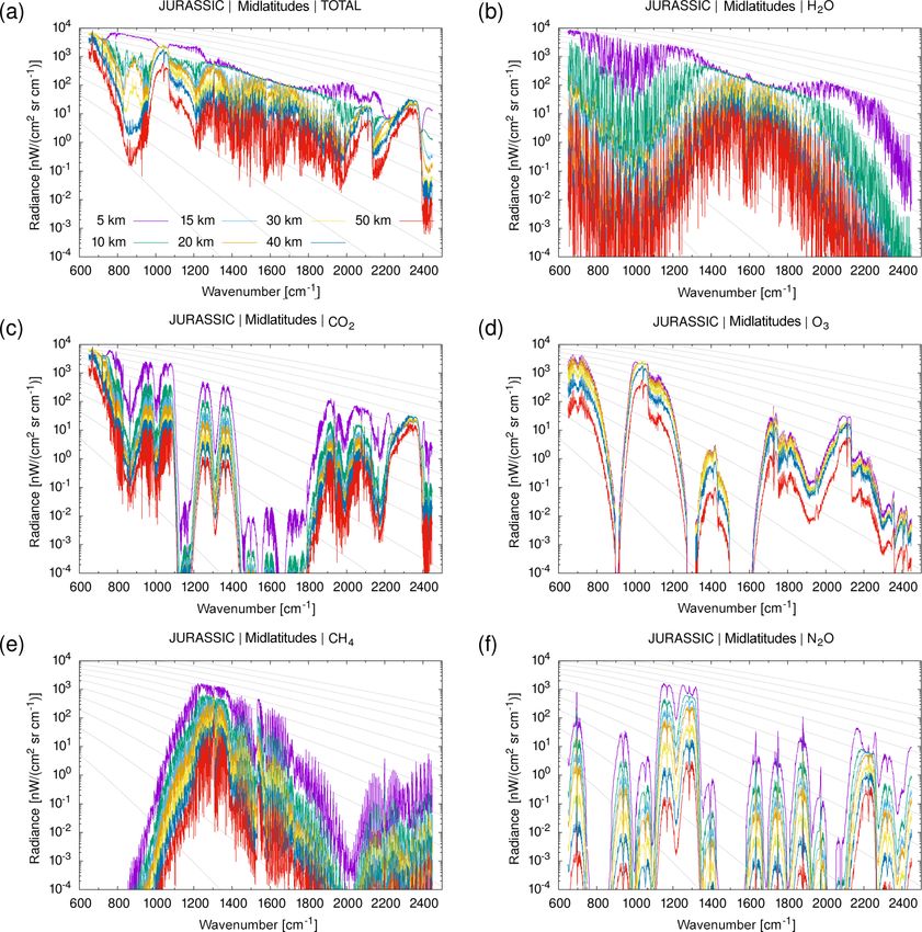
In the study of Baumeister et al. (2017), we analyzed the
CO2 H2 O N2 O2 Number of
registers
performance of the GPU implementation of JURASSIC for
nadir applications. Here, we selected the limb geometry as
0 0 0 0 77 a test case (see Fig. 6). While in the nadir geometry ray
0 0 0 1 82 paths typically comprise 160 path segments (assuming an up-
0 0 1 0 84 per height of the atmosphere at 80 km and default vertical
0 0 1 1 84
sampling step size of 500 m), the limb geometry produces
0 1 0 0 87
up to about 400 segments per ray path. Ray paths passing
0 1 0 1 92
0 1 1 0 94 only through the stratosphere feature fewer segments than
0 1 1 1 94 ray paths passing by close to the surface. Tropospheric ray
1 0 0 0 78 paths are also subject to stronger refractive effects, bending
1 0 0 1 82 them towards the Earth’s surface. In the limb test case consid-
1 0 1 0 84 ered here, the number of segments along the ray paths varies
1 0 1 1 84 between 122 and 393.
1 1 0 0 87 In this assessment, we aim for rather extensive coverage
1 1 0 1 92 of the mid-infrared spectral range. By means of line-by-line
1 1 1 0 94 calculations with RFM, we prepared emissivity look-up ta-
1 1 1 1 94
bles for 27 trace gases with 1 cm−1 spectral resolution for the
range from 650 to 2450 cm−1 . Vertical profiles of pressure,
temperature, and trace gas volume mixing ratios for midlat-
counts allow for a larger degree of parallelism and, poten- itude atmospheric conditions were obtained from the clima-
tially, a higher throughput. tological data set of Remedios et al. (2007).
In order to verify the model, we continuously compared
3.2 Verification and performance analysis GPU and CPU calculations during the development and op-
timization of JURASSIC-GPU. For the test case presented
3.2.1 Description of test case and environment in this study, it was found that the GPU and CPU calcula-
tions do not provide bit-identical results. However, the rel-
In the following sections, we discuss the verification and ative differences between the calculated radiances from the
performance analysis of the JURASSIC-GPU code. All per- GPU and CPU code remain very small (≤ 10−5 ), which is
formance results reported here were obtained on the Jülich orders of magnitudes smaller than typical accuracies of the
Wizard for European Leadership Science (JUWELS) super- EGA method itself (∼ 1 %) and considered suitable for most
computing system at the Jülich Supercomputing Centre, Ger- practical applications.
many (Krause, 2019). The JUWELS GPU nodes comprise a
Dual Intel Xeon Gold 6148 CPU and four NVIDIA Tesla
https://doi.org/10.5194/gmd-15-1855-2022 Geosci. Model Dev., 15, 1855–1874, 2022You can also read