EUROVISION SONG FESTIVAL MELODY GENERATION - UVA SCRIPTIES
←
→
Page content transcription
If your browser does not render page correctly, please read the page content below
Eurovision song festival melody
          generation.
              Bachelor thesis

                   Lex Johan
                   12181242

        Bachelor Kunstmatige Intelligentie

            University of Amsterdam
               Faculty of Science
               Science Park 904
             1098 XH Amsterdam

                   Supervisor
               Dr. J.A. Burgoyne
       Faculteit der Geesteswetenschappen
       Capaciteitsgroep Muziekwetenschap
           Nieuwe Doelenstraat 16-18
              1090 BB Amsterdam

                   April, 2021

                        1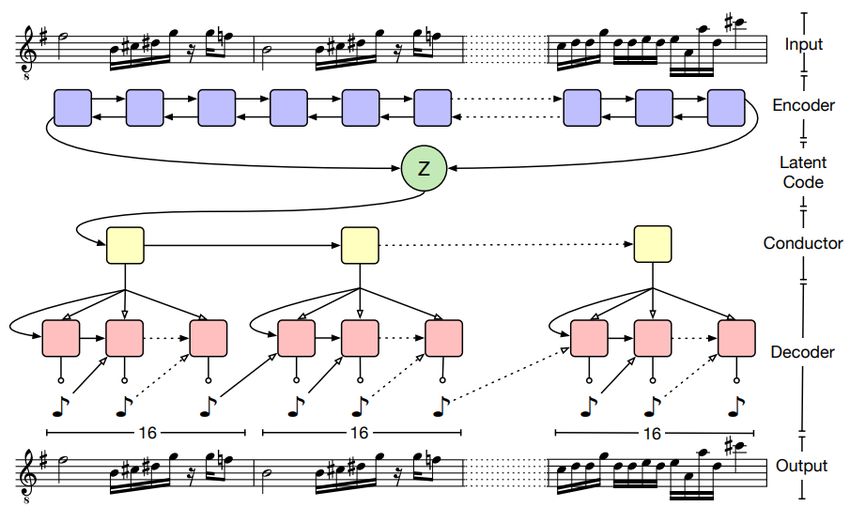
Abstract
  The research question that this thesis will try to answer is: “What quality of
melody are state-of-the-art music generation artificial intelligent algorithms able
to produce based on Euro vision song festival songs”. To achieve this, live audio
   recording have been turned into MIDI files to train three neural networks:
  Melody RNN, MusicVAE and MidiNet. These models were compared to one
 another both objectively and subjectively through a user study. Both of these
comparisons agree that MusicVAE is able to make the best melodies out of the
                                     three.

                                        2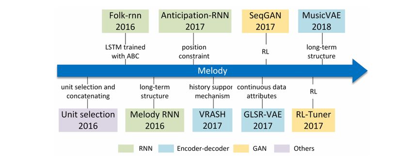
Contents

1 Introduction                                                                                                                            4

2 Background                                                                                                                              6
  2.1 Variational autoencoder (VAE) . . . .                              .   .   .   .   .   .   .   .   .   .   .   .   .   .   .   .    6
  2.2 Generative adversarial network (GAN)                               .   .   .   .   .   .   .   .   .   .   .   .   .   .   .   .    6
  2.3 Long short-term memory (LSTM) . . .                                .   .   .   .   .   .   .   .   .   .   .   .   .   .   .   .    7
  2.4 Convolutional neural network (CNN) .                               .   .   .   .   .   .   .   .   .   .   .   .   .   .   .   .    7

3 Related work                                                                                                                            8
  3.1 Melody generation      .   .   .   .   .   .   .   .   .   .   .   .   .   .   .   .   .   .   .   .   .   .   .   .   .   .   .    8
  3.2 MusicVAE . . . . .     .   .   .   .   .   .   .   .   .   .   .   .   .   .   .   .   .   .   .   .   .   .   .   .   .   .   .   10
  3.3 MidiNet . . . . . .    .   .   .   .   .   .   .   .   .   .   .   .   .   .   .   .   .   .   .   .   .   .   .   .   .   .   .   11
  3.4 Melody RNN . . .       .   .   .   .   .   .   .   .   .   .   .   .   .   .   .   .   .   .   .   .   .   .   .   .   .   .   .   12

4 Method                                                                                                                                 13
  4.1 Dataset . . . . . . . . . . . . . . . . . . .                               . . . . .          .   .   .   .   .   .   .   .   .   13
  4.2 Preprocessing . . . . . . . . . . . . . . . .                               . . . . .          .   .   .   .   .   .   .   .   .   13
      4.2.1 Segmentation (SBIC) . . . . . . . .                                   . . . . .          .   .   .   .   .   .   .   .   .   13
      4.2.2 Melody extraction (MELODIA) . .                                       . . . . .          .   .   .   .   .   .   .   .   .   14
      4.2.3 bpm estimation (Multi-feature beat                                   tracker)            .   .   .   .   .   .   .   .   .   14
      4.2.4 Melody frequency to MIDI file . . .                                   . . . . .          .   .   .   .   .   .   .   .   .   15
  4.3 Training the models . . . . . . . . . . . . .                               . . . . .          .   .   .   .   .   .   .   .   .   15

5 Results                                                                      16
  5.1 Objective comparison . . . . . . . . . . . . . . . . . . . . . . . . . . 16
  5.2 Subjective comparison . . . . . . . . . . . . . . . . . . . . . . . . . 18

6 Conclusion and discusion                                                                                                               21

                                                     3
Chapter 1
Introduction
The goal of artificial intelligence (AI) has long been to emulate human intelligence,
and a part of that intelligence is our creativity. Computational creativity is a mul-
tidisciplinary field that tries to obtain creative behaviors from computers. One of
its most prolific subfields is that of music generation (also called algorithmic com-
position or musical meta-creation), which uses computational means to compose
music. This process of automatically generating new musical pieces is particularly
hard for many reasons, for example, there is no loss function to test the quality of
the music generated. Furthermore, what does good quality music mean to human
listeners? These questions will not be answered any time soon, but researchers
have made many strides in the last decade.
The goal of music generating systems is sometimes to create a formalization of
a certain musical style, like Bach. Other times, the generation of music itself is
the only goal. These diverging goals also lead to diverging methods, each with its
strengths and weaknesses. Not all these methods use AI in the sense of an artificial
neural network (ANN). Some try to approach music as if it was a natural language
with formal grammars, while others try to solve the problem of music generation
with genetic algorithms.
This thesis will focus on melody generation based on live Eurovision audio
files of 1593 songs from 1956 to 2020, in an attempt to create ’pleasant-sounding’
melodies. To achieve this, three types of ANNs will be compared with each other:
a convolutional neural network generative adversarial network (Yang et al. 2017),
a recurrent neural network with long short-term memory (Waite 2016), and a
variational autoencoder (Roberts et al. 2018). To evaluate the quality of music
generation, people will be asked to state a preference among melodies created
through the three ANNs. The research question that this thesis will try to answer
4is: “What quality of melody are state-of-the-art music generation artificial intelli-
gent algorithms able to produce based on Euro vision song festival songs”.
5Chapter 2
Background
This is a quick overview of the different kinds of ANNs that have been used in this
thesis with their major characteristics.
2.1 Variational autoencoder (VAE)
A VAE (Kingma & Welling 2019) is a type of unsupervised ANN which can learn
the representation or encoding of the input data. It consists of three major parts:
the encoder, the latent space and the decoder. The latent space acts as a bottleneck
between the encoder and decoder, forcing the model to ignore the insignificant data
to learn the representation. The training steps for this type of model are as follows:
The input data is encoded as a distribution over the latent space, from this latent
space a point can be sampled to be decoded, this allows the reconstruction loss to
be calculated which can be back propagated through the model.
2.2 Generative adversarial network (GAN)
A GAN (Creswell et al. 2018) consists of two types of networks: a generator and
a discriminator. The generator is trained to produce new samples from the input
data, while the discriminator is trained to distinguish between real samples data
and generated samples. These two models are trained together in a zero-sum game,
which is halted when the generator is able to recover the training data and the
discriminator is able to distinguish between real and generated samples 50% of the
time.
62.3 Long short-term memory (LSTM)
LSTMs (Hochreiter & Schmidhuber 1997) are a special kind of recurrent neural
networks (RNN), which allow information to persist like memory. RNNs can use
this memory to process sequences of variable lengths as input. However, RNNs
suffer when learning long-term dependence (Bengio et al. 1993), where the interval
between the relevant information and the current state of the input sequence has
become too large. LSTMs were introduced to combat this issue and are capable of
remembering values over arbitrary time intervals. A LSTM unit contains: a cell,
an input gate, an output gate and a forget gate. These components work together
to control the flow of information into and out of the cell.
2.4 Convolutional neural network (CNN)
CNNs (O’Shea & Nash 2015) utilize convolutions to capture the spatial and tem-
poral dependencies of an image. A convolutional kernel is repeatedly applied to the
input image, which results in a feature map detailing the locations and strengths
of a detected feature in the input image. The strength of CNNs lies in the fact that
they are capable of automatically learning a large amount of these convolutional
kernels in parallel.
7Chapter 3
Related work
3.1 Melody generation
Music generation is far from a new idea, going as far back as the 1960s (Ames
1987). Research in this area has not stalled since then, and many new methods
have been created with the goal of music generation. However, with the advent
of machine learning, new life has been blown into this field. These recent models
utilize state-of-the-art techniques used in the other domains of machine learning,
for example, transformer models primarily used in natural language processing
tasks have also been adapted to music generation (Huang et al. 2018). This thesis
focuses on a sub-domain of music generation: melody generation, which is much
simpler because these models only have to predict the probability of a single note
at each time step. A few popular models in melody generation from the past five
years are detailed below in figure 3.1.
Figure 3.1: Chronology of melody generation. (Ji et al. 2020)
8According to Ji et al. (2020), these kinds of models face three major challenges:
structure, closure and creativity. Structure in melodies are recurring themes, mo-
tivations, and patterns, these are often lacking in the output of the models which
make the melodies boring. Closure is the sense of conclusion that follows from any
tension created in the melody (Hopkins 1990), since these models lack any control
over when the melodies will, there will always be a lack of closure. Lastly, cre-
ativity in melody generation is the ability to create new melodies not found in the
dataset, however, contemporary machine learning techniques are mainly capable
of interpolation of the training dataset and therefore unable to truly come up with
something new.
93.2 MusicVAE
MusicVAE (Roberts et al. 2018) follows the basic structure of VAEs for sequential
data proposed in Bowman et al. (2015), however, it tries to solve the challenge
of structure with their unique hierarchical decoder. For their encoder, they use
a two-layer bidirectional LSTM network with a state size of 2048 for both layers,
which feeds into the latent space with 512 dimensions.
In their preliminary testing, they found that using a simple RNN as the decoder
would result in the loss of long-time structure in the generated melodies. This was
hypothesized to be caused by the vanishing influence of the latent space as the
output sequence was generated. To alleviate this issue, the authors came up with
the ’conductor’, which is a two-layer unidirectional LSTM with a hidden state size
of 1024 and 512 output dimensions. This conductor uses the latent vector to create
embeddings, which through a tanh activation layer serve as initial states for the
bottom-layer decoder. The decoder consists of a two-layer LSTM with 1024 units
per layer. An overview of this model can be found in figure 3.2
Figure 3.2: Schematic overview of the MusicVAE model.
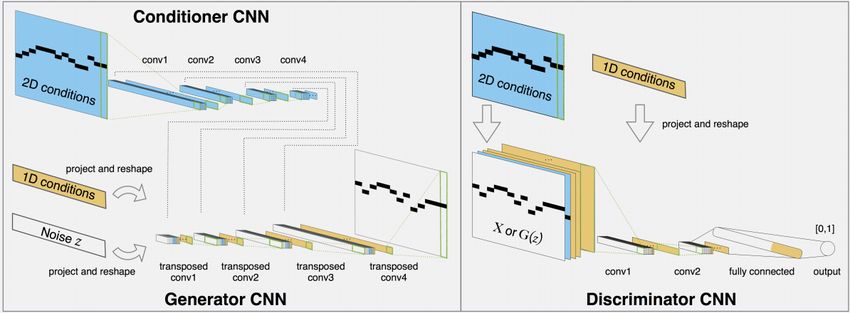
103.3 MidiNet
MidiNet presents a GAN CNN-based model that takes advantage of the symbolic
domain generation of melody. Instead of creating a continuous melody sequence,
MidiNet proposes to generate melodies in a successive manner. This is achieved by
converting the MIDI sequence of notes into a two-dimensional matrix representing
the presence of notes over time in a bar and employing convolutions over this
matrix. Furthermore, to promote the creativity displayed by the network, random
noise is used as input to the generator part of MidiNet.
This generator’s goal is to transform the random noises into two-dimensional
score-like representations which should resemble real MIDI sequences. The gen-
erator uses a special convolution operator called transposed convolution, which
“up-samples” smaller matrices or vectors to larger ones. The output of the gener-
ator is given to a discriminator, which has to learn to distinguish between which
of its inputs are from real MIDI files and which of its inputs are from the genera-
tor. Together, this generator and discriminator pair form the GAN, but this GAN
alone does not ensure the temporal dependency between the different bars which
this model claims to do.
MidiNet resolves this by introducing a conditional mechanism to use music
from the previous bars to condition the generation of the current bar. To do this,
a separate CNN model has to be trained, which is referred to as the conditioner.
Using this conditioner, MidiNet has the ability to look back at its previously
generated bars without the use of recurrent units, as is done in music generation
models using RNN techniques.
Figure 3.3: Schematic overview of MidiNet
113.4 Melody RNN
Melody RNN (Waite 2016) consists of two methods to improve a basic RNN’s
ability to learn longer-term structures: Lookback RNN and Attention. The first
method, Lookback RNN, in addition to inputting the previous event in the se-
quence as a normal RNN would, it can look back 1 and 2 bars to recognize patterns
such as mirrored or contrasting melodies. Furthermore, the position within the
measure is also used as an input, allowing the model to more easily learn patterns
associated with 4/4 time music.
The second method, Attention RNN, builds upon the basic RNN by imple-
menting a mechanism of attention as found in Bahdanau et al. (2014). Attention
is a different approach in ANNs to access previous information without having to
store it in an RNN cell’s state. In this implementation, the amount of attention
the last n steps receive from the current step will determine how much of their
activation is concatenated with the output of the current cell.
12Chapter 4
Method
4.1 Dataset
The dataset used to train all four models consists of all 1593 Eurovision Song
Contest songs in the period of 1956 to 2020 in the form of MP3 live audio files.
The total duration of play time is around 88 hours, which includes introductory
talks and Charpentier’s ’Te Deum’ as opening theme in certain years. Both of
these have to be removed in later preprocessing steps.
4.2 Preprocessing
To train the models, the live audio recordings need to be turned into the symbolic
music format MIDI. A four-part data preprocessing pipeline was constructed to
achieve this.
4.2.1 Segmentation (SBIC)
The live audio recordings still contain the introductory talks and opening themes
in certain years, these had to be removed to achieve the best possible result in
the melody extraction in the next step. To accomplish this, the SBIC algorithm
(Gravier et al. 2010) from the Python Essentia library (Bogdanov et al. 2013)
was utilized, this algorithm segments audio using Bayesian information criterion
given a matrix of feature vectors. For this use case, the Mel-frequency cepstrum
coefficients (MFCCs) were used as feature vectors, since the MFCCs of either
an introductory talk or ’Te Deum’ are sure to differ greatly from the rest of the
song. The algorithm then searches for homogeneous segments in which the feature
vectors have the same probability distribution.
134.2.2 Melody extraction (MELODIA)
To convert the live audio recordings to MIDI, the fundamental frequency has to be
extracted. This was accomplished with the MELODIA algorithm (Salamon et al.
2013) from the Essentia library, the working of this algorithm can be summarized
in four parts: sinusoidal extraction, a salience function, pitch contour creation and
the melody selection. The sinusoidal extraction takes the frequencies present in
the live audio recordings and transforms them using the discrete-time short-time
Fourier transformation to compute the prevalence of each frequency.
The output of this transformation acts as the input for the salience function,
the goal of this function is to estimate the pitches from the frequencies in each
moment of time. For all possible pitches (within a reasonable range) a harmonic
series is sought which contributes to our perception of that pitch. The weighted
sum of the energy in these harmonic frequencies can be referred to as the ’salience’
of that pitch, this is repeated for each time step in the audio.
The peaks of the salience function at each time step can be used to track the
pitch contours, these are a series of consecutive pitch values which are continuous in
both time and frequency. Any outliers left after this step are removed in the melody
selection, and we are left with an approximation of the fundamental frequency of
the audio and thus its melody.
This algorithm is focussed on the melody produced by the singer’s voice, mean-
ing the generated melody will fall silent when the singer’s voice cannot be detected.
4.2.3 bpm estimation (Multi-feature beat tracker)
For the construction of MIDI files, a bpm estimation is necessary. This was
achieved through the multi-feature beat tracker algorithm (Oliveira et al. 2012)
from the Essentia library, which utilizes the mutual agreement of five different fea-
tures to estimate the bpm of the input audio: complex spectral difference, energy
flux, spectral flux in MFCCs, a beat emphasis function and spectral flux between
histotgrammed spectrum frames.
144.2.4 Melody frequency to MIDI file
Given a frequency f of a melody in a certain time step, the corresponding MIDI
note d can be found with:
$ !'
f
d = 69 + 12 log2 (4.1)
440
Applying equation 4.1 over all frequencies in the melody and with the estimated
bpm, it is possible to create a MIDI file.
These steps were combined in the processing pipeline summarized below in
figure 4.1, after preprocessing, the total amount of playtime in the MIDI files was
reduced to around 81 hours.
Figure 4.1: Overview of preprocessing pipeline
4.3 Training the models
These MIDI files cannot be used directly in the training of the ANNs, however, the
models’ respective GitHub repositories all contain tools to convert MIDI files to
the correct format. Furthermore, all models were trained with their recommended
parameters for the recommended number of epochs.
15Chapter 5
Results
5.1 Objective comparison
The aesthetics of music cannot be measured by a computer, however, it is possible
to compare the outputs of the different models in an objective manner through the
features in the MIDI files. To compare these models, each model had to generate
10 melodies, each with a length of 30 seconds. As a control group, the MIDI files
from the melody extraction can be used.
Figure 5.1: Distribution of number of pitch classes. the Models appear on the
x-axis and the number of pitch classes appears on the y-axis.
Firstly, there is the distribution of the total number of pitch classes from each
model in figure 5.1. Melody RNN immediately jumps out with the highest devia-
16tion, while the control group centers clearly on 15 pitch classes, both MidiNet en
MusicVAE fall in between these two results. If there are too few different pitch
classes in the output, it will result in a boring melody, while too many different
pitch classes can result in a lack of cohesion. The fact that Melody RNN displays
both behaviors could mean that this ANN was unable to learn anything significant.
The control group also displays remarkable behavior with its small deviation, but
this could also be the result of the melody extraction.
Figure 5.2: Distribution of average pitch range per melody. the Models appear on
the x-axis and the average pitch range appears on the y-axis.
Secondly, there is the distribution of the average pitch range in figure 5.2. This
number is calculated by the subtraction of the highest and lowest used pitch in
semitones. Melody RNN is an outlier here as well, with the control and MusicVAE
having a much smaller deviation. MidiNet also comes close to the control group.
A too low pitch range could result in a boring melody, while a too high pitch range
could indicate a chaotic melody. Again, Melody RNN displays both behaviors just
as in figure 5.1, but the control group also display similar behavior as in figure 5.1.
17Figure 5.3: Distribution of the average pitch shift. the Models appear on the x-axis
and the average pitch shift appears on the y-axis.
Finally, we have the distribution of the average pitch shift in figure 5.3. This
number is calculated as the average value of the interval between two consecutive
pitches in semitones. Melody RNN again has by far the largest deviation, however,
this time MidiNet comes closest to the control group while MusicVAE is deviates
more. Here as well, Melody RNN is on both ends of the spectrum, but MusicVAE
has the highest mean average pitch shift, possibly pointing towards more chaotic
melodies generated by this model.
5.2 Subjective comparison
The aesthetic qualities of the music were measured with a user study. Fifteen
Participants each had to listen to 30 seconds of melody per ANN and a melody
out of the training data. They were asked to score three questions in Dutch
between one and seven. These questions can be translated as follows: 1. How
pleasant is the melody to listen to? 2. How is the cohesion of the melody? And
3. How interesting is the melody? The results are as follows:
18Figure 5.4: Distribution of answering scores for the control group
The results for the control group are quite high across the board as seen in figure
5.4, with question one and two both a higher mean score of 4 points, however these
melodies were lacking interesting aspects according to the participants
Figure 5.5: Distribution of answering scores for Melody RNN
The results for Melody RNN are much lower, as seen in figure 5.5, never reach-
ing a higher mean than three points and even a mean of two points on question
two. The lack of cohesion, which the participants have voted on in question 2, is
in line with the objective comparisons made earlier. This could also explain the
low scores on the other two questions.
19Figure 5.6: Distribution of answering scores for MidiNet
The results for MidiNet as seen in figure 5.6 are quite average, while it scores
above average on question one with a mean of 4 points, the deviation on question
3 is quite high.
Figure 5.7: Distribution of answering scores for MusicVAE
The results for MusicVAE as seen in figure 5.7 are the highest outside the con-
trol group, with all mean scores higher than 4 points. It even scores higher than
the control group on whether the melody is interesting
From both the results of the objective and subjective comparisons, the Mu-
sicVAE is the winner. Melody RNN is lower on the spectrum of the subjective
comparison, but this is in line with the objective comparison in section 5.1.
20Chapter 6
Conclusion and discusion
The question posed in the introduction of this thesis:“What quality of melody are
state-of-the-art music generation artificial intelligent algorithms able to produce
based on Euro vision song festival songs”. To this end, a processing pipeline was
made to turn the live audio performances into viable training data for three kinds
of ANNs. The generated melodies were both put through objective and subjective
comparisons, highlighting their differences. Melody RNN is the clear loser of this
comparison in both perspectives, despite the promises of long-time structure that
LSTMs bring with them, however, Melody RNN is also by far the simplest model
of the three. But the fact remains that there is enough evidence to say that Melody
RNN unable to learn anything significant from the data.
Second in place is MidiNet, which scored average in subjective comparison and
did not stand out in the objective comparison, while the participants overall agree
that the melody is pleasant, they were more divided on whether the melody was
interesting.
Finally, there is MusicVAE, which has scored comparatively high on the sub-
jective comparison and was very similar to the control group in the objective
comparison. Most remarkable is that this model was able to create more inter-
esting melodies than the control group according to the participants of the user
study. Perhaps this can also be seen in figure 5.7 where the distribution of the
average pitch shift is higher than the other models and the control group.
To improve on the results found in this thesis, the hyperparameters of both the
models and the MELODIA algorithm could be tweaked. The latter is especially
important because the training data was far from perfect, in future work the
processing pipeline should contain a step which removes long silences which are
left after the MELODIA algorithm.
21Bibliography
Ames, C. (1987), ‘Automated composition in retrospect: 1956-1986’, Leonardo
pp. 169–185.
Bahdanau, D., Cho, K. & Bengio, Y. (2014), ‘Neural machine translation by jointly
learning to align and translate’, arXiv preprint arXiv:1409.0473 .
Bengio, Y., Frasconi, P. & Simard, P. (1993), Problem of learning long-term de-
pendencies in recurrent networks, pp. 1183 – 1188 vol.3.
Bogdanov, D., Wack, N., Gómez Gutiérrez, E., Gulati, S., Boyer, H., Mayor, O.,
Roma Trepat, G., Salamon, J., Zapata González, J. R., Serra, X. et al. (2013),
Essentia: An audio analysis library for music information retrieval, in ‘Britto
A, Gouyon F, Dixon S, editors. 14th Conference of the International Society
for Music Information Retrieval (ISMIR); 2013 Nov 4-8; Curitiba, Brazil.[place
unknown]: ISMIR; 2013. p. 493-8.’, International Society for Music Information
Retrieval (ISMIR).
Bowman, S. R., Vilnis, L., Vinyals, O., Dai, A. M., Jozefowicz, R. & Ben-
gio, S. (2015), ‘Generating sentences from a continuous space’, arXiv preprint
arXiv:1511.06349 .
Creswell, A., White, T., Dumoulin, V., Arulkumaran, K., Sengupta, B. & Bharath,
A. A. (2018), ‘Generative adversarial networks: An overview’, IEEE Signal Pro-
cessing Magazine 35(1), 53–65.
Gravier, G., Betser, M. & Ben, M. (2010), ‘Audioseg: Audio segmentation toolkit,
release 1.2’, IRISA, january .
Hochreiter, S. & Schmidhuber, J. (1997), ‘Long short-term memory’, Neural com-
putation 9(8), 1735–1780.
Hopkins, R. G. (1990), Closure and Mahler’s Music: The Role of Secondary Pa-
rameters, University of Pennsylvania Press, pp. 4–28.
URL: http://www.jstor.org/stable/j.ctv5138cg.5
22Huang, C.-Z. A., Vaswani, A., Uszkoreit, J., Shazeer, N., Hawthorne, C., Dai,
A. M., Hoffman, M. D. & Eck, D. (2018), ‘Music transformer: Generating music
with long-term structure’, arXiv preprint arXiv:1809.04281 .
Ji, S., Luo, J. & Yang, X. (2020), ‘A comprehensive survey on deep music genera-
tion: Multi-level representations, algorithms, evaluations, and future directions’,
arXiv preprint arXiv:2011.06801 .
Kingma, D. P. & Welling, M. (2019), ‘An Introduction to Variational Autoen-
coders’, arXiv e-prints p. arXiv:1906.02691.
Oliveira, J. L., Zapata, J., Holzapfel, A., Davies, M. & Gouyon, F. (2012), ‘As-
signing a confidence threshold on automatic beat annotation in large datasets’.
O’Shea, K. & Nash, R. (2015), ‘An introduction to convolutional neural networks’,
arXiv preprint arXiv:1511.08458 .
Roberts, A., Engel, J., Raffel, C., Hawthorne, C. & Eck, D. (2018), A hierarchical
latent vector model for learning long-term structure in music, in ‘International
Conference on Machine Learning’, PMLR, pp. 4364–4373.
Salamon, J. J. et al. (2013), Melody extraction from polyphonic music signals,
PhD thesis, Universitat Pompeu Fabra.
Waite, E. (2016), ‘Generating long-term structure in songs and stories’.
URL: https://magenta.tensorflow.org/2016/07/15/lookback-rnn-attention-rnn
Yang, L.-C., Chou, S.-Y. & Yang, Y.-H. (2017), ‘Midinet: A convolutional gener-
ative adversarial network for symbolic-domain music generation’.
23You can also read


