Elephants or Goldfish?: An Empirical Analysis of Carrier Reciprocity in Dynamic Freight Markets
←
→
Page content transcription
If your browser does not render page correctly, please read the page content below
Elephants or Goldfish?:
                                               An Empirical Analysis of Carrier Reciprocity in Dynamic Freight Markets
                                                                         Angela Acocella, Chris Caplice, Yossi Sheffi
                                                        MIT Center for Transportation & Logistics, 1 Amherst St. Cambridge, MA 02142

                                               Abstract
                                               Dynamic macroeconomic conditions and non-binding truckload freight contracts enable both
                                           shippers and carriers to behave opportunistically. We present an empirical analysis of carrier reci-
arXiv:2108.07348v1 [q-fin.GN] 4 Aug 2021

                                           procity in the US truckload transportation sector to demonstrate whether consistent performance
                                           and fair pricing by shippers when markets are in their favor result in maintained primary carrier
                                           tender acceptance when markets turn. The results suggest carriers have short memories: they do
                                           not remember shippers’ previous period pricing, tendering behavior, or performance when mak-
                                           ing freight acceptance decisions. However, carriers appear to be myopic and respond to shippers’
                                           current market period behaviors, ostensibly without regard to shippers’ previous behaviors.
                                                   Keywords: truckload freight transportation, tender acceptance, market cycles

                                           1       Introduction
                                           In the US freight transportation industry, shippers (e.g., manufacturers, wholesalers, distributors,
                                           or retailers with goods to be moved) and carriers (transportation service providers such as trucking
                                           companies that move those goods) interact constantly. These interactions between the two actors
                                           become important contributors to overall logistics costs. Over-the-road transportation moves ap-
                                           proximately 10 billion tons of freight per year (Costello, 2018) and accounted for 4.3% of the $19
                                           trillion US GDP in 2017. The two for-hire trucking options available to shippers are full truckload
                                           (TL) - large shipments, typically over 10,000 pounds, where the shipper is usually the sole customer
                                           - and less-than-truckload (LTL) - smaller shipments that cannot fill an entire trailer where multiple
                                           shippers’ loads are consolidated together. For-hire TL transportation spend totaled $296.1 billion
                                           in 2018, or 44.3% of over-the-road freight transportation (AT Kearney, 2018).
                                                As a result of deregulation of the industry following the 1980 Motor Carrier Act, shippers
                                           have followed two approaches to procure for-hire TL transportation. They can enter into long-
                                           term contracts with carriers or seek capacity on the spot market. To procure contracted capacity,
                                           shippers conduct a reverse auction1 . They forecast expected annual transportation demand for
                                           each lane (origin-destination pair) within their freight distribution networks, decide if and how to
                                           package lanes together in order to make them more attractive to carriers, and invite carriers to
                                           participate by issuing a Request for Proposals (RFPs). Carriers respond to RFPs by stating the
                                           price they are willing to accept to serve each lane. This price is based on origin and destination
                                           characteristics (e.g. expected dwell time or likelihood of obtaining a follow-on load after drop-off),
                                           expected volume (number of loads offered per week), the carriers’ operating costs, fleet size, and
                                           existing network. The shipper typically selects the lowest bidding carrier with which to enter a
                                           contract, subject to some level of service constraints; this is the primary carrier. Under these
                                           contracts, prices are set and held exclusively and privately between shippers and carriers, typically
                                           lasting one or two years. (See Caplice (2007) for a detailed discussion of the TL transportation
                                           procurement process).
                                               1
                                               In a reverse auction, rather than the buyer responding to the seller with his willingness to pay for the good or
                                           service, the seller of the good or service responds to the buyer with the price she is willing to accept.

                                               Please cite this article as Acocella, Caplice, Sheffi, "Elephants or Goldfish?: An Empirical Analysis of
                                                 Carrier Reciprocity in Dynamic Freight Markets", Transportation Research Part E: Logistics and
                                                  Transportation Review, Vol 142, 2020, https://doi.org/10.1016/j.tre.2020.102073. ©2020 This
                                                             manuscript version is made available under the CC-BY-NC-ND 4.0 license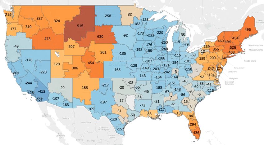
As an alternative to contracted services, shippers can have immediate demand served on the spot
market - an open marketplace where prices are determined on a load-by-load basis and shippers and
carriers are matched for individual load transactions. Typically, about 72% of for-hire TL freight
is accepted by primary carriers, while only 6% is fulfilled by spot capacity (Aemireddy and Yuan,
2019). As the industry evolved post deregulation, both shippers and carriers sought relationships
with one another to encourage better performance and pricing consistency (Crum and Allen, 1991;
Gibson et al., 1993).
    These relationships are difficult to ensure, however, as the terms of the contract between shippers
and primary carriers are non-binding in terms of volume and frequency commitments. This is a
unique quality of TL transportation as compared to the procurement of other services. When
shippers and carriers enter long-term contracts, for each origin and destination pair (lane), only
the price at which the carrier agrees to provide services is binding; there is no hard and fast
commitment on the shipper’s part to offer loads to the carrier. Nor is there any commitment on
the carrier’s part to accept all loads when offered.
    To address potential primary carrier load rejections, shippers compile a routing guide, consisting
of an ordered list of backup carriers that had responded to the shipper’s RFP. Typically these
carriers’ bid prices (i.e. price at which they indicated willingness to serve the lane) are higher
than that of the chosen primary carrier. If a load is rejected by the primary carrier, the shipper’s
transportation manager consults the routing guide and offers the load to an alternate carrier,
which again can accept or reject the load. In the case of the alternate carrier rejection, the shipper
continues down the routing guide until one of the backup carriers accepts the load. If the routing
guide fails, the shipper must turn to the spot market. Backup carriers’ prices indicated during
procurement are not binding as contracted carriers’ are, and these backup carriers may demand
higher prices if they are called upon later. Aemireddy and Yuan (2019) find that on average,
backup carrier prices are 9-12% higher than contract prices, depending on routing guide depth,
while average spot rates exceed contract prices by 23-35%, depending on market conditions.
    The non-binding agreements further complicate planning long-term budgets and services accu-
rately for both parties. The problems are compounded as shippers procure transportation services
from many carriers across their distribution networks and carriers serve many shippers (Caplice
and Sheffi, 2003, 2005). Shippers must balance trade-offs between pricing, expected transportation
service levels, and their own customer demand uncertainty, while carriers face a dynamic pickup
and delivery problem in which they face random demand and short lead times as their trucks move
from point to point (Powell et al., 1988; Berbeglia et al., 2010)2 .
    These issues worsen when macroeconomic factors are considered. The freight transportation
industry undergoes market fluctuations due to changes in the overall economy, hedging or otherwise
opportunistic pricing during the transportation procurement process, truck driver shortages or
churn, regulations, and extreme weather events (Pickett, 2018). In what is referred to as a soft
market, the demand for transportation services is less than available trucking capacity, driving
prices down and carriers to accept only marginally profitable or even unprofitable freight – this is
when shippers hold the more advantageous position. On the other hand, in a tight market, demand
for transportation outstrips supply, carriers have their pick of freight they want to move, prices are
high, and carriers have the advantage. The most recent cycle from soft to tight market occurred
around Q3 2017 (Pickett, 2018), and markets began to soften again around the Q4 2018.
    A key performance indicator used by shippers is a primary carrier’s acceptance ratio (PAR) -
that is, the fraction of loads the carrier accepts relative to the number of loads that it is offered
   2
     See Williamson (1993, 1985) for a detailed discussion of the trade-offs and implications of contract economics
and relational contracts.

                                                        2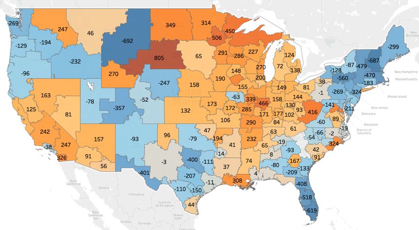
by the shipper on a lane a carrier has won as primary carrier. When a primary carrier’s PAR
declines, as is seen in tight periods, shippers must go deeper in their routing guides to find non-
contracted carriers to move their loads. Elevated freight rejection and high transportation costs in
tight market periods hinders overall business performance (Smith, 2019). As a result, during tight
periods shippers search for ways to develop relationships with their carriers and ensure consistent
performance through the cycle, seeking ‘shipper of choice’ status, (C.H. Robinson, 2015).
    The tensions between shippers and carriers that we highlight motivate this study, in which we
test the often-heard opinion by shippers and carriers that they each “have long memories” between
market cycles.
2     Literature Review
A vast set of literature related to the PAR problem models the load matching and carrier assignment
decisions to help shippers and carriers improve performance. Due to advances in near-real-time
data availability and computational capabilities, much of the recent literature has explored dynamic
versions of these problems, where the shippers’ load information becomes available over time rather
than being known a priori. A related, but much smaller body of literature studies shipper-carrier
relationships.
2.1    Strategic carrier assignment decisions
Two problems in the transportation literature, which are related but distinct, are the shipper’s
strategic decision during the procurement process of which primary carrier to assign to each lane,
and the operational decision regarding which carrier to offer each load.
    Caplice (1996) and Caplice and Sheffi (2003) argue that economies of scope come about when
shippers and carriers make procurement and bid decisions by considering their network as a whole
rather than on a lane-by-lane basis. A combinatorial optimization approach to the procurement
auction is developed to improve efficiencies; in particular, to improve how carriers communicate
their cost function information to shippers and how shippers assign carriers to lanes. These studies
focus on the bids that carriers submit in response to the RFP and develop formal optimization
models and solutions for how shippers should analyze these submissions and assign carriers to lanes.
    Building on this research, Lu (2003) considers both bid cost and carrier reputation in the
shipper’s combinatorial carrier assignment problem. The author finds that when taking reputation
into account during the primary carrier selection process, shippers pay more in total direct costs
to carriers, but there is a decrease in total hidden costs, which results in a net savings in total
transportation costs. Including carrier reputation in the assignment decision is also considered
by Rekik and Mellouli (2012). Here, the reputation-based winner determination problem where
allocation of long-term contracts to carriers is decided based on both bid ask prices and carriers’
reputation. The carriers’ reputation is translated into unexpected hidden costs the shipper may
incur when working with the winning carriers.
    The above literature assumes the shipper has decided to outsource the transportation service
and models the shipper’s selection of for-hire carriers. However, a number of studies have ap-
proached the carrier assignment problem in which the shipper chooses between contracting for-hire
carriers and serving the lanes itself with a private fleet. This set of literature includes Guastaroba
et al. (2009), Caplice et al. (2011), Lee and Po (2007), and Mulqueen (2006). For a review of the
TL transportation service procurement modeling approaches including contract or spot agreements
between shippers and carriers, the reader is referred to Basu et al. (2015).

                                                  3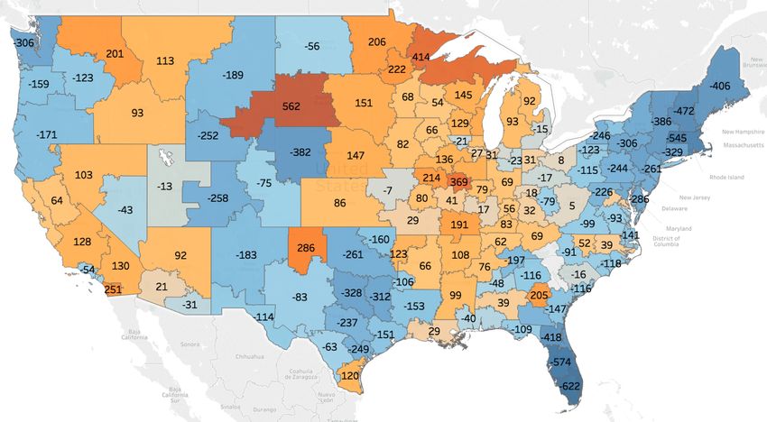
2.2   Operational load matching decisions
The load assignment problem finds the minimum-cost assignment of loads to carriers, where each
load must be picked up at a given location at a specific time and delivered to a known destina-
tion (see Powell et al. (1995)). Powell (1996) presents a methodology to evaluate the dynamic
load assignment model with demand uncertainty and real time information using rolling horizon
simulations.
    Similarly, simulation approaches have been applied to study the dynamic nature of TL load
matching operations by Tjokroamidjojo et al. (2006) and Regan et al. (1998). Further, Simão
et al. (2009) demonstrate an approximate dynamic programming method to accurately simulate
the operations of the largest truckload motor carrier in the US, with over 6,000 drivers. The
authors make use of both pre- and post-decision states in order to deal with the complexities of
carriers’ operations. The model includes driver attributes such as home domicile, desire to be offered
loads that get them back home, and hours already worked. Load attributes including origin and
destination, appointment and delivery types, and revenue, are also included to allow the company
to test the value of changes in the mix of drivers, freight, and other operating policies. The authors
highlight that their model can be extended to help the carrier make tender acceptance decisions at
the load level based on the current state of the system and ultimately evaluate how to commit to
contractual agreements with shippers.
2.3   Shipper-carrier relationships
The S-C relationship as it relates to market conditions and the nature of the resulting contractual
agreements is the focus of Hubbard (2001), which studies relationship-specific investments in the
trucking industry. The author argues that in trucking, the customer (i.e., shipper) rarely expe-
riences asset specificity - that is, investments specific to partners (carriers) over long horizons as
compared to other industries. He argues that with increasing long-haul trucking market thickness
- that is, as more buyers and sellers come to the market - shippers and carriers utilize simple spot
transactions rather than more complicated contractual arrangements.
    Much of the extant transportation literature on shipper-carrier (S-C) relationships relies on
surveys, interviews, and isolated experiments rather than empirical industry data, in part due to
the difficulty of obtaining private company data. Carriers’ freight acceptance has been the focus of
a few studies based on transaction data, however. Rather than measures of the S-C relationship,
most authors consider attributes of the lanes and freight in determining whether a load will be
accepted. High lane volume (Harding, 2005), low lane volume volatility (Kim, 2013), high pricing
(Amiryan and Bhattacharjee, 2015), and high lane consistency, or cadence, (Aemireddy and Yuan,
2019) have been found to be positively correlated with higher primary carrier AR (PAR).
    The S-C relationship, however, has been found to contribute to carriers’ freight acceptance in
a few studies. Zsidisin et al. (2007) find that contracted carriers, which shippers believe represent
good relationships, outperform carriers that demonstrate poor or purely transactional relationships
in terms of freight acceptance, on-time delivery, and pre-positioned capacity.
    Scott et al. (2017) analyze contract and spot market transactions and the impact the S-C
relationship on freight acceptance. They find that less frequent load offers increase the likelihood of
a carrier rejecting a load, while higher offered volume, lower load offer volatility, and higher revenue
transacted between the shipper and carrier increase the likelihood of carrier’s load acceptance. The
authors do use a measure of market condition - Spot Premium - which is the ratio of 7-day average
spot prices to 7-day average contract prices in a geographic region. As the unit of analysis in the
model is at the load level, this rolling ratio still indicates immediate market conditions, testing
whether carriers are more or less likely to accept loads in one market or another. We extend this

                                                   4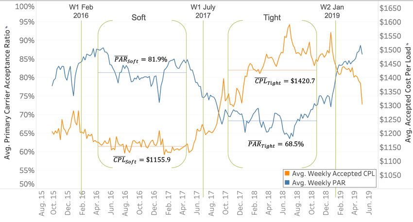
market condition consideration by including previous market behaviors into the acceptance decision
model.
    Each of these studies utilizes data from a single shipper, which limits their ability to generalize
across types of shippers or to segment the data by S-C relationship types. Moreover, while the
above literature explores the S-C relationship and its effects on carriers’ tender acceptance, it does
not consider previous behaviors explicitly defined by market conditions. Our research contributes
to the TL transportation literature in that we analyze transactions and behaviors between many US
shippers and contracted carriers and determine how the relationship between them in one market
condition corresponds to performance in the next, when power dynamics have shifted.
3     Research Question and Hypotheses
To address the research gaps described above, we formulate the following research question, which
considers the degree to which shippers and primary carriers stand by the terms of their previously
defined non-binding contracts as market conditions (and power dynamics) change:

RQ: Should shippers pay competitive prices or provide high, consistent freight vol-
umes when markets are soft to ensure carriers will adhere to contract expectations
when the market tightens with high acceptance ratios of contracted loads?

    In particular, do carriers have long memories (thus, act like elephants) and reciprocate high soft
market period pricing, tender consistency, or high volume from shippers with consistent, high PAR
in tight periods? Conversely, do carriers reciprocate low soft period pricing, tender consistency,
or volume from shippers with lower tight period PAR? Or, do carriers act like goldfish with short
memories, forgetting shippers’ previous behaviors?
    In short, our research question considers whether it is worth it for a shipper to “pay it forward”
by strictly adhering to contract commitments even when lower cost options may be available. This
we measure with primary carrier acceptance ratio and formulate the following hypotheses:
3.1    Carriers’ response to previous shipper behavior
First, we focus our attention on whether carriers respond to shippers’ previous behaviors. That
is, do carriers have long memories (thus, act like elephants) and reciprocate good performance
soft market from shippers with high PAR in tight periods? We measure “good” performance as
competitive pricing, consistent tendering patterns, advanced load notice, minimal delays at pick-up
and delivery, and frequent business. We consider asset-based primary carriers independently from
non-asset primary carriers (which, in our context includes brokers serving as contracted carriers), as
they may have different strategies, access to capacity, and perhaps tolerances for certain customer
behaviors. This leads us to the following two hypotheses:
    H1a: Asset-based primary carriers offer high tight market period PAR for their shippers that
had demonstrated good performance in the previous soft market period.
    H1b: Non-asset primary carriers offer high tight market period PAR for their shippers that
had demonstrated good performance in the previous soft market period.
3.2    Carriers’ response to current shipper behavior
Second, we consider whether carriers respond to shippers’ current behaviors. That is, do carriers
act more like goldfish and offer high tight market PAR for shippers demonstrating current good
behaviors? Thus, we formulate the following two hypotheses:
    H2a: Asset-based primary carriers offer high tight market period PAR for their shippers that
demonstrate good performance in the current tight market period.

                                                  5
H2b: Non-asset primary carriers offer high tight market period PAR for their shippers that
demonstrate good performance in the current tight market period.
4 Methodology
In the following section, we describe the hybrid break point detection method implemented for
this study, define the market time periods, characterize the S-C pairs and describe the model we
implement to answer our research question.
4.1 Empirical Data Summary
The data for this research is obtained from a partner company that provides logistics and trans-
portation functions for its shipper clients. Our partner company is not a brokerage, but rather is
a managed services provider assisting its clients (shippers). The relationship and all payments are
directly between the shipper and the carrier with no intermediaries. This is important to note,
as we intend to study the direct relationship between a shipper and its primary carriers, not how
carriers interact with a third party. Many companies offer such managed transportation services.
For example, Transplace, BluJay Solutions, 4Flow, C.H. Robinson, and XPO Logistics. While the
latter firms are two of the largest traditional 3PL providers in the US, they both offer independent
managed transportation services as described above without promoting or relying on the brokerage
side of their businesses.
For our purposes, we obtain both tactical pricing information and operational load transaction
data. The carriers’ pricing information is obtained during each shippers’ procurement event; prices
carriers bid for each lane are collected, one or more carriers are selected to be contracted, and a
subset of the remaining carriers that bid are retained as backup carriers in cases where the primary
carriers reject loads. Typically this process is either done solely by the client shipper, or with the
help of our partner company, depending on the the shipper’s needs. This pricing information for
each carrier - primary (i.e., contracted) and all backup (i.e., non-contracted) - is uploaded into the
routing guide, which we obtain from our partner company.
The provided data further includes transactions for all of the client shippers’ TL loads that
originate and terminate within the continental United States, each loads’ corresponding carrier
tender sequence beginning with the primary carrier through any backup carriers if needed and each
carriers’ acceptance or rejection decisions until a carrier finally accepts the load.
After data cleaning and pre-processing, we retain just under four years of transactions; from
September 2015 to May 2019. In particular, the data spans one complete market cycle into the
next - that is, a soft period, a tight period, and the beginning of a second soft period, which are
defined and tested in §4.2. For consistency, we consider only TL, dry van, long haul (greater than
250 miles) loads, since pricing schemes differ for other freight types and shorter lengths of haul.
As a result, we maintain 1,933,299 unique loads offered by 71 shippers, tendered to 1,650 primary
carriers. They comprise 7,573 shipper-primary carrier pairs operating from 4,915 origin 5-digit zip
codes to 9,668 destination 5-digit zip codes. The dataset also contains geographic regions defined
by our industry partner as key economic zones of shippers’ business. The continental United States
is divided into a set of 135 mutually exclusive and collectively exhaustive regions. Each of these
regions represents an origin and a destination region.
Table 1 below summarizes the data set. In addition to these variables, the metrics described in
the following subsections are computed to measure attributes of the S-C relationship.
6Table 1: Data Summary
Date range Sept 1, 2015 - May 30, 2019
Shipment Type TL, dry van, long haul (≥250 mi)
Num. Loads 1,933,299
Num. Shippers 71
Industries Automotive, Food & Beverage or Con-
sumer Package Goods, Manufacturing, Pa-
per & Packaging, Other
Num. Primary Carriers 1,640
(Asset-based: 1,446, Non-asset: 194)
Num. Shipper-(Primary)Carrier pairs 7,573
Num. Origin 5-digit Zips (Regions) 4,915 (135)
Num. Destination 5-digit Zips (Regions) 9,668 (135)
4.2 Break Point Detection and Market Period Definition
First, we define the market periods by detecting breaks in market data. The time series of aggre-
gated weekly PAR across all shippers is used as a proxy for market conditions. Previous literature
(Scott et al. (2017), Scott (2015), and Kirk (2013), for example), use monthly spot market prices
to characterize market conditions. In our dataset only about 2% of the total transactions go to the
spot market and this value changes with market conditions as more loads go to the spot market
during tight periods, As such, our data is limited in using spot prices to define market periods as
other studies have.
However, Scott et al. (2017) show a 77.3% correlation between spot premium time series data
and the Morgan Stanley supply and demand sentiment index, which surveys a broad array of
shippers, carriers, and brokers. Our weekly national PAR series and this same Morgan Stanley
weekly freight index from 2015 to 2019 have a correlation of -85.2%. That is, we show that high
demand for capacity correlates with lower PAR - the definition of a tight market. Not only are
supply and demand over time strongly correlated with spot prices as demonstrated in Scott et al.
(2017), we show that they are strongly correlated to our measure of the market, PAR. Thus we can
be confident in choosing PAR rather than other metrics (e.g., spot prices, freight industry indices
such as national load-to-truck ratio, truck manufacturing order rates, or other macroeconomic
indicators) to define market conditions; acceptance ratios capture real-time carrier decisions.
In practice, many shipper monitor the changing market conditions by tracking the PAR along
with outer routing guide failures – not just spot market price changes. In fact, one could argue that
PAR is a more sensitive metric than spot premium as it captures contract abandonment by carriers.
Thus, PAR is an appropriately representative and sensitive measure of how carriers respond to and
communicate with shippers and, thus, of overall market conditions. Further, by considering the
aggregate measure, the break points detected do not presuppose this study’s results.
To define and validate the identified breaks, we combine two distinct break point detection
methods. As neither method perfectly captures the changes we expect, we run each method inde-
pendently and take points that are identified by both methods as validated breaks. This results in
a more robust break point detection method.
4.2.1 Quandt Algorithm
The Quandt method, developed by Chow (1960) and expanded by Quandt (1960) is the standard
econometric test for a break point that is not known a priori. The method calculates a sequence
7of Pearson’s chi-square statistics to determine when the series has shifted (Hansen, 2001). The
algorithm considers each point in the time series as a candidate break point, τ . The data is split
into sub periods at τ : A for t ≤ τ , and B for t > τ . We estimate the vector of coefficients of a
linear regression fit to each sub period and to the full series without a break (denoted by T):
ŷtA = β̂0A + β̂1A XtA + εA , t≤τ
ŷtB = β̂0B + β̂1B XtB + εB , t>τ (1)
ŷtT = β̂0T + β̂1T XtT T
+ε , ∀t
The chi-square distribution is used to assess the statistical significance of the difference between
the two regression models and the equality of the coefficients is tested using an F -statistic (the
ratio of two chi-square distributions) (Chow, 1960; Hansen, 2001).
The break point, τ̂ , is determined to be the point at which the maximum Fτ is achieved:
τ̂ = argmaxτ Fτ
Typical F -statistic critical values for such tests are not appropriate for Fτ̂ when the break point
is not known a priori and the Quandt method is applied (Hansen, 2001). However, critical value
tables for the Quandt statistic and p-value calculation methods have been developed by Andrews
(1993), Andrews and Ploberger (1994), and Hansen (1997).
The Quandt algorithm described above considers all points in the time series for which τ ∈
[τ0 , τ1 ], where we exclude the tails of the data from consideration as candidate points to maintain
enough observations on either side to estimate meaningful regression models (Quandt, 1960; Hansen,
2001). The sample is trimmed to the interior λ to (1−λ) range of the data. Hansen (2001) suggests
that typical values of the trimming parameter, λ, fall between 0.05 and 0.15. In this study we use
λ = 0.05 trim and address its sensitivity by defining a transition period on either side of a detected
break point when defining our market periods.
4.2.2 Considerations of the Quandt Algorithm
While well documented in econometric and statistics literature, the Chow and Quandt algorithms
have a number of drawbacks when applied to the data presented in this paper. First, the methods
are well suited for time series data containing a single break, and despite extensions developed to
account for multiple breaks, the results of these extensions are sensitive to both the date range and
the trim parameter selected.
The second drawback of the Quandt algorithm as applied to this research is that it tests for
locations in which one can fit the best linear model to each segment of the data. However, that is
not the intent of this step in our research. We merely require a method to determine when average
values of the aggregated PAR has changed. Unfortunately, break point detection based on average
values is not found extensively in the literature. As such, we combine the method described above
with a sequential difference of means test described in the following subsection.
4.2.3 Jumping Mean Approach
We are interested in determining the times at which the average value of the aggregated PAR
changes. To identify these points, for each date in the time series, τ , we compute the average of the
PAR values for the preceding W weeks and the following W weeks. These backward- and forward-
b,W f,W
looking average values are denoted by X τ and X τ , respectively and we take the absolute value
of the difference between the two values, DτW :
b,W f,W
DτW = |X τ − Xτ | (2)
8Where
W −1
b,W 1 X
Xτ = Xτ −i
W
i=0
(3)
W
f,W 1 X
Xτ = Xτ +i
W
i=1
In doing so, we draw from a data mining context, which describes such a ‘jumping mean’ break
point measure, where a break is detected if a difference score (which we define here as the absolute
difference in means between the forward- and backward-looking window of the data) is large enough
(Takeuchi and Yamanishi, 2006). We consider the points at which the local maxima of the absolute
difference occur as potential break locations, as suggested by Hansen (2001) and Bai (1997) for the
Quandt method.
Next, applying a standard t-test, we check the statistical significance of the difference of means
at the potential breaks, τ . If tstat > tcrit at the desired significance level we consider it as a potential
break point.
We test the sensitivity of this combined method to the window size, W . Windows of 6, 10,
12, 26, 34, and 52 weeks are tested and we determine that a satisfactory window size is 12 weeks,
as smaller windows are too sensitive to variability in the data, detecting many immaterial break
points, and larger windows over-smooth, missing potentially important breaks (see Appendix A for
window sensitivity test results).
Next, we combine the results of the Quandt algorithm and this jumping mean approach. We
retain only break dates that are identified by both the Quandt method and the jumping mean
approach with a 12-week window. These dates are summarized in Table 2. The resulting validated
break points are the first week of February 2016, the first week of July 2017, and the second week
of January 2019 (see Figure 1).
Table 2: Break points identified by the Quandt method and jumping mean approach
Quandt results Jumping mean
02-05-16 02-07-16
05-29-16
01-29-17
06-28-17 06-25-17
09-02-18
01-16-19 01-20-19
4.2.4 Market Period Definitions
While determining a break at a single point is simple and convenient, claiming that an economic
market change takes place at a single specified date is not realistic. We use the break point
detection method described above as a first order approximation of a structural change point
(Hansen, 2001). To account for seasonal effects, we take a full year of data for each defined time
period. By selecting a full year during each market period we average out any seasonality individual
shippers or industries observe. In this way, seasonality in demand for distinct shippers or industries
in one market period is compared to the same seasonality in the second market period and allows
us to compare across shippers of different size and industry. Further, in order to allow for market
transition buffer time, we choose the year of data that is centered between our validated break
dates.
9While it is reasonable to consider economic markets as continuous rather than discrete as we
do here, we define our research question such that we measure market-specific behaviors, and
thus must define market periods. To procure transportation services, shippers typically run annual
national bid events, which are essentially seen as step changes resulting in rates and primary carrier
agreements that are expected to be in effect for a year. These step change, which represent how
the shipper is responding to the current market conditions, occur are different times throughout
the year for different shippers. The result of cumulative shipper annual bids eventually leads to
a distinct market type. Moreover, the decision to discretize the market is based on conversations
with industry practitioners, who tend to refer to distinct “soft” and “tight” market periods. Our
resulting market periods are defined in Table 3 below.
Table 3: Market Periods
Soft Tight
Date Range Apr. 15, 2016 – Apr. 14, 2017 Oct. 1, 2017 – Sept. 30, 2018
Avg. Weekly PAR 81.9% 68.5%
Avg. Weekly CPL $1155.9 $1420.7
Figure 1 shows both the average weekly aggregated PAR and the average weekly accepted
cost per load (CPL) over time overlaid with our identified break points and market periods. This
CPL is the linehaul price that is accepted, which includes primary carriers, backup carriers within
the routing guide, and spot loads. The two measures mirror each other as expected: as the
market tightens, acceptance ratios decrease and prices paid increase. As the market softens again,
acceptance ratios increase and accepted prices decline.
Figure 1: Validated Break Dates, Market Periods, Aggregated Primary Carrier Acceptance Ratio
(PAR) (left axis), and Accepted Cost Per Load (right axis)
104.3 S-C Relationship Measures
We select and define the S-C relationship metrics based on a combination of relationship attributes
studied in the inter-firm relationship literature and in TL transportation literature, TL transporta-
tion industry reports, and conversations with our industry partner and with professionals at both
shipper and carrier organizations. Thus, we have developed a set of relationship characteristics
based in both theory and practice.
We define the relationship between shippers and carriers along six shipper behaviors measured in
each of the market periods, The first, Primary carrier Acceptance Ratio (PAR), in the tight market
is our dependent variable in our model. The remaining set of shipper behaviors is composed of
pricing relative to market rates, volatility of volume offered measured, tender lead time, and origin
and destination dwell times. In addition, we include one characteristic of S-C interactions across
time periods (cadence of tenders), two shipper characteristics (size and industry), and two carrier
characteristics (fleet size and asset- versus non-asset). We detail these measures in the following
subsections and report summary statistics in Appendix C.
4.3.1 Primary carrier Acceptance Ratio
Primary carrier Acceptance Ratio (PAR)3 is measured as the weekly fraction of loads that are
accepted by the primary contract carrier relative to the total number of loads offered to that
carrier from a specific shipper:
a,b
La,b
i,j,w,accepted
P ARi,j,w = (4)
La,b
i,j,w,of f ered
where L is the number of loads either accepted or offered; a and b denote the shipper and
carrier, respectively; i and j denote the origin and destination regions, respectively; and w is the
week in which loads are offered.
High PAR in a soft period does not necessarily indicate a good S-C relationship because demand
is low in soft markets and carriers search for business regardless of their relationship with shippers.
On the other hand, low PAR in a soft period is a signal of a poor S-C relationship, as it is in the
portion of the market cycle when carriers need loads. On aggregate, PAR decreases as the market
turns from soft to tight, by definition of the market types. However, we expect that S-C pairs
with an existing strong relationship will not experience a decrease in PAR as severe as that of the
aggregate market PAR decline.
We calculate PAR for a S-C pair on each of their lanes, and in each week in which loads are
offered between them. This value is averaged over all weeks in each of the market periods and
we obtain an average weekly acceptance ratio, which is averaged again across all lanes between a
a,b
shipper and carrier in each market period to obtain the S-C PAR for both periods: P ARsof t and
a,b 4
P ARtight .
4.3.2 Market Rate Differential
Market Rate Differential (MRD), or the percent above or below market benchmark prices at which
a load moves, measures how much of a premium (or discount) a shipper pays its primary carrier.
As noted earlier, we expect that shippers paying high soft period prices, when the market is in their
3
Primary carrier AR (PAR) is a preferred measure to AR across all carriers, where the same load may be rejected
multiple time.
4
We do not weight the PAR by volume offered, number of weeks in the year loads are offered, or number of lanes
between the S-C pair. As a result, the relative importance of each load is higher for S-C pairs with less total volume
(or fewer weeks or lanes) than that of S-C pairs with more volume (or weeks or lanes).
11favor, will receive better performance in the next tight period - that is, carriers reciprocate high
soft period pricing with high tight period PAR. On the other hand, we expect shippers that pay
low soft market prices are taking advantage of their position and carriers respond with decreased
PAR in the following tight period.
We determine MRD by calculating a benchmark price for each lane against which the S-C pairs’
contract prices are to be compared. Our load data is split into the soft and tight periods to obtain
lane benchmark rates for each time period. Freight transportation costs can be reduced to a linear
combination of fixed costs and variable costs associated with a distance measure (Daganzo, 2005).
The benchmark rate captures the regional nature of TL pricing with lane-specific fixed effects by
including origin and destination indicator variables. In doing so, we incorporate effects of outbound
loads from the origin and inbound loads to the destination. These factors are important as carriers
makes load acceptance decisions, in large part based on where they have available capacity, where
they will ultimately end up, and the likelihood of obtaining follow-on loads.
We implement a multiple linear regression model with heteroskedastic robust standard errors
in which the load linehaul price is regressed on an origin region indicator variable, a destination
region indicator variable, and distance variable (Ballou, 1991; Scott, 2015).
Specifically, an indicator variable is created for all but one of the origin regions and all but
one of the destination regions. The lane which corresponds to this origin-destination pair is the
base case lane. The base case origin and destination regions are chosen based on their outbound
and inbound volume, respectively. We measure the total outbound (inbound) volume in both of
the time periods, t ∈ {Sof t, T ight}, for each region. The base case origin (destination) region is
chosen if it is ranked in the top five regions by volume in both time periods. If more than one
region qualifies, we take the region with the highest cumulative volume. We choose a high-demand
lane as our base case to ensure it is representative of aggregate market conditions.
Our resulting base case origin region is the greater Greenville, SC area and the base case
destination region is the Dallas, TX metro region. We test this choice of base case origin and
destination regions among top-ranked regions by volume and find that the differences between lane
benchmark values relative to one another for varying base case regions do not impact statistical
results.
The vector of coefficients that results from our linear regression includes an intercept term,
which is the fixed transportation cost, β̂base t t , I-1
, a distance (i.e. variable cost) coefficient, β̂dist
origin coefficients (where I is the set of origin regions in the dataset), and J-1 destination coefficients
(where J is the set of destination regions in the dataset). These 135 key economic regions defined
by our industry partner are geographic clusters of transportation demand patterns. The origin
and destination coefficients of our linear regression model, β̂it and β̂jt , can be considered ‘price
premiums’, or the costs associated with an origin or destination different from the base case lane.
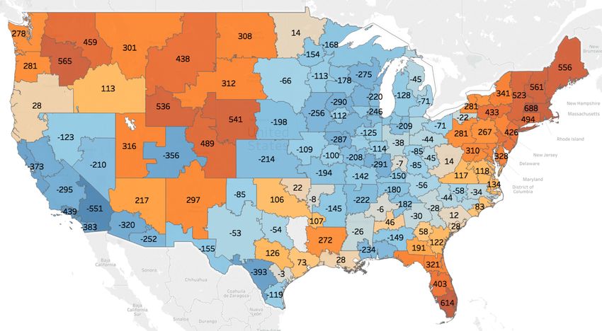
The origin and destination price premiums, β̂it and β̂jt , for each time period, are illustrated in
t
Appendix B, as are β̂base t . In general, relative pricing of the regions hold through market
and β̂dist
periods. For example, in both the soft and tight markets, the Midwest and Southwest regions of the
United States are typically higher priced regions to ship out of (i.e. positive and high origin price
premiums). This is likely due to the large manufacturing hub in the Midwest the port authorities
of Los Angeles and Long Beach causing high demand for outbound capacity. As a result, carriers
can command higher prices. At the same time, the Northeastern region does not generate much
freight volume relative to the rest of the country; carriers are willing to take lower prices in order
to leave the region (i.e. negative origin price premiums in the Northeast), whereas higher prices are
required to incentivize inbound carriers in the first place (demonstrated by high destination price
premiums in the Northeast). Thus, these regional values define and quantify fore and backhaul
12lanes.
Each lane benchmark rate is calculated as follows. The base case lane benchmark price is
t
the regression model intercept, β̂base t , multiplied by the mean
, plus the distance coefficient, β̂dist
value of the distance variable of loads on that specific origin-destination pair, X dist . All other lane
benchmark rates consist of the fixed cost intercept term, plus the distance coefficient and variable
interaction, plus the origin and destination region coefficient price premiums corresponding to that
lane, β̂it and β̂jt :
X X
b̂ti,j = β̂base
t t
+ β̂dist X dist + β̂it Xi + β̂jt Xj (5)
i∈I,i6=ibase j∈J,j6=jbase
where Xi and Xj are binary variables indicating which origin and destination is active for the
lane of interest. Once the lane benchmark rates are established, the market rate differential is
calculated per load, k, as the percent above or below the lane benchmark price. That is, the
difference between the load linehaul price and the corresponding lane benchmark rate, relative to
the benchmark rate:
t
LHk,a,b − b̂ti,j
t
M RDk,a,b = (6)
b̂ti,j
t , by averaging over all loads on
We obtain the market rate differential for a S-C pair, M RDa,b
each lane between the shipper and carrier, and averaging across all of their lanes for each market
period separately.
In the next subsections we discuss shippers’ operational performance that may impact the S-C
relationship and thus carrier reciprocity in tight market conditions. A natural measure may be the
the total business offered to the carrier. However, the total amount of volume a shipper tenders
to a carrier does not necessarily lead to better carrier performance, as the business offered must
fit the carrier’s network. For example, previous literature on the benefits of information sharing
finds two seemingly opposing results. In a dyadic supply chain, Helper et al. (2010) demonstrate
that supplier capacity limits the value of sharing information. However, Bakal et al. (2011) show
that the benefit of information sharing is lower with suppliers with less capacity. As such, we use
consistency (or CV, volatility), tender lead time, offer cadence as operational measures of good
shipper tendering behavior rather than pure volume tendered.
4.3.3 Tendered volume volatility
TL carriers commonly call for consistency of demand at the load and lane levels. For the shipper,
this means minimizing variation in tendering behaviors. Industry reports from J.B. Hunt, one of
the largest TL carriers in the US, and C.H. Robinson, a leading third party logistics (3PL) provider
in the US, cite increased consistency as an action shippers can take to improve their relationships
with carriers, improve freight acceptance, reduce cost per load, and allow carriers and their drivers
to better optimize profitability (J.B. Hunt (2015) and C.H. Robinson (2015)). Further, previous
studies find consistency measures to be significant indicators of spot market load acceptance (Scott
et al., 2017), reduced cost per load (Harding, 2005), and reduced routing guide failure (Aemireddy
and Yuan, 2019).
We measure variability of volume tendered by a shipper as the coefficient of variation (CV)
of the weekly volume offered. This normalized measure indicates what percent of the mean the
standard variation is. It is used rather than raw standard deviation in order to compare the
variability measure across dissimilar lanes. A shipper with high tendered volume variability is
expected to have low PAR because inconsistency causes difficulty for carriers’ network planning.
13As a result of high variability, either trucks will not be available when and where shippers need
them, or carriers will not make an effort to ensure these inconsistent shippers are served. Thus, we
expect that higher volatility from shippers leads to lower PAR in tight markets.
4.3.4 Tender lead time
In order for carriers to balance capacity utilization with availability, they need enough time to
respond to the tender requests, ensure a truck is available, and reposition it to the pickup location on
time. According to J.B. Hunt, in addition to consistency and predictability, carriers seek reasonable
lead times, which allow them to create a schedule and optimize driver’s hours (J.B. Hunt, 2015).
For example, Caldwell and Fisher (2008) found that with greater tender lead time, a shipper saw
lower variability in prices paid for loads. We measure this tender lead time (TLT) as the number
of days between when the load is first offered to the primary carrier to when it needs to be picked
up.
It is important to note however, that with too many days of advanced notice, much can change
in that time. For example, the appointment time may need to change, the carrier may not have
capacity available as expected because of previous service delays, or the shipper may have been
tendering the load to gather information of general carrier availability or willingness to serve for
the tendered price. This point is illustrated by the numerical results of Zolfagharinia and Haughton
(2014), which find that with a two-day TLT, the carrier’s profit increases 22% over the base case
of one day, but three days of advanced load notice only increases the carrier’s profit by 6% over
the base case. Lindsey et al. (2015) and Scott (2015) study the impact of lead time on spot
prices. The former consider a dummy variable for loads with greater than 8 days of lead time,
while the latter finds that the impact of lead time drops off quickly for TLT longer than two days.
Tjokroamidjojo et al. (2006) model the benefit of advanced load information sharing (i.e., TLT) to
minimize carrier’s total cost and find that carriers seek longer TLT. However they do not address
the potential non-linearity in benefit from increased TLT addressed by some of the other studies.
4.3.5 Origin and destination dwell time
Carriers are often concerned with delays that occur during pickup and delivery. In a study of
shipper behaviors that impact carrier performance C.H. Robinson (2015) finds that carriers cited
dwell times in their top shipper characteristics important to price and service decisions. Dwell
time becomes even more important when one considers the regulations drivers face in terms of
hours of service (HOS) laws5 . Particularly in times when capacity is tight and carriers want to
retain drivers, drivers’ time utilization goes hand in hand with asset utilization and thus, carriers’
attitudes toward shippers J.B. Hunt (2015).
Dwell time is also considered in the literature; Zolfagharinia and Haughton (2014) and Tjokroamid-
jojo et al. (2006) include dwell time in their modelling approaches as a cost incurred by carriers.
Delays during delivery can often be more problematic than pickup because drivers may be able
to make up some of that added time during the move. However, delays at the destination may
make the driver late to the next job’s appointment, which may then add further delays to that
pickup, thus, proliferating the problem. We expect then, that destination dwell times may have
higher impact on PAR than that at origins.
5
In essence, a driver has 14 hours of “on-duty” time with a required 30-minute break. 11 of those 14 hours can be
spent driving and 2.5 hours can be spent on all other activities, including pickup, delivery, safety inspections, and
shutdown. However, it is not uncommon for live loading and unloading to take longer than 2.5 hours. When these
activities do, it eats into the drivers’ precious 11 hours of “on-duty, driving” time they could otherwise be using to
make a profit.
144.3.6 Offer cadence
In line with carriers’ desire for consistency and the ability to plan for demand, the frequency, or
cadence, at which shippers tender loads is often attributed to carrier’s freight acceptance. In a
general supplier-customer setting, Rinehart et al. (2004) study inter-firm behaviors and argue that
interaction frequency is a key success factor to supplier-customer relationships. Scott et al. (2017)
includes the number of days since the previous load was offered to a spot carrier by a shipper as a
measure of load offer frequency. Interviews with practitioners and industry reports by J.B. Hunt
and C.H. Robinson demonstrate that tender cadence, as measured by weeks in which loads are
offered to the carrier, is a measure carriers use to assess shipper relationship (J.B. Hunt (2015) and
C.H. Robinson (2015).
We measure frequency at which a shipper offers loads to a carrier as the number of weeks in
a year in which the shipper offers at least one load to its primary carrier. We compare a metric,
offer cadence, or the percentage of weeks during the year in which the shipper tenders loads to its
primary carrier. For individual S-C pairs in our dataset, this percentage for the soft period and
the tight period are highly correlated (with correlation coefficient of 0.90) so we use an average
measure across the two market periods. Shippers that offer loads more frequently are expected to
receive higher PAR, as the carriers rely on frequent loads to move trucks around their network and
ensure trucks are available in the right location and at the right time for the portfolio of shippers
served.
Table 4 summarizes the S-C attributes we consider and the literature and the academic and
industry reports that have previously considered such attributes. This is not meant to be a com-
prehensive list, but a subset of the literature most closely related to our research question at hand.
Table 4: S-C Relationship Metrics in the Literature
Study PAR Pricing Volatility TLT Dwell Cadence
Aemireddy and Yuan (2019) X X X
Caldwell and Fisher (2008) X X
C.H. Robinson (2015) X X X X
Harding (2005) X X X
J.B. Hunt (2015) X X X X
Kim (2013) X X X
Lindsey et al. (2015) X
Rinehart et al. (2004) X
Scott (2015) X X
Scott et al. (2017) X X X X
Tjokroamidjojo et al. (2006) X X
Zolfagharinia and Haughton (2014) X X
Zsidisin et al. (2007) X
Finally, as the main focus of our study is to examine the impact of shipper behaviors and
market conditions on tight market PAR, we control the impact of other factors that characterize
the shippers and the carriers, described below.
4.3.7 Shipper and carrier characteristics
In this section, we describe the attributes of the shippers and carriers themselves that we include
in our model to control for fixed effects. This allows us to determine if certain types of shippers
15or carriers behave or experience impacts from market changes differently from others. These fixed
effects include shipper size, shipper industry, carrier size, and carrier service type.
Shipper size: Previous S-C relationship literature has been limited in the scope of available
shipper data, however our dataset consists of hundreds of shippers. Thus, we contribute to the
literature by considering the impacts of shipper characteristics. First, we consider the shipper’s
size, which we measure as the log (base 10) of average total annual volume tendered to all primary
carriers. Larger shippers may be better insulated from the impacts of the market and maintain
better carrier relationships. On the other hand, smaller shippers may invest in relationships with
a smaller core set of carriers, and thus have better carrier relationships. We test if a shipper’s sizes
impacts how it experiences carrier performance as the markets shift.
Shipper industry: We similarly utilize the granularity of our available data by including the
shipper’s industry vertical in our model. Each shipper falls into only one of six industry categories:
automotive, food & beverage or consumer package goods (F&B/CPG), manufacturing, paper and
packaging, or a final catch-all category, other.
Carrier fleet size: Carriers with different attributes operate - and thus make decisions -
differently. We first consider asset-based carriers’ fleet size, measured as the log (base 10) of the
carrier’s tractor count, as an indicator of tight market PAR. For smaller carriers such as the single
truck owner-operator, or those with only a few trucks, when demand is very high as is seen in tight
markets, accepting tendered volume becomes more difficult than for larger carriers, as these small
carriers have fewer available trucks to cope with the additional demand.
Carrier service type The second carrier attribute we consider is the carrier’s service type.
We split our data into S-C pairs for which the primary carrier is an asset-based carrier, which
can be further segmented by fleet size as describe above, and a second set for which the primary
carrier is a non-asset provider such as a brokerage. These providers do not own trucks, yet they
may be contracted with shippers to provide services in a similar way to the asset carriers. Instead,
they match their contracted shippers’ needs with a vast pool of available capacity composed of
many carriers. Brokerages utilize their extensive network of disagragate capacity to tailor the
shipper-carrier match to the needs of both parties.
We are aware of one study that considers the differences in behaviors between asset and non-
asset carriers, specifically, on spot load pricing strategies (Scott, 2018). The author uses auction
theory to address the differences in how asset and non-asset carriers consider the two main decisions
made in auctions - whether and how much to bid. He finds that non-asset carriers bid more
frequently and higher than their asset counterparts. This study, one of the few empirical studies
of actual firms’ decisions repeated auctions over time as the author claims, underscores our claim
that asset-based carriers and non-asset carriers behave differently and justifies our consideration of
them separately.
In our dataset, the non-asset carrier for these S-C pairs is defined as the brokerage itself, not
the carrier that ultimately matched and moved the load. That is, we do not have visibility on
which trucking company actually moved the load. Thus, we can characterize the shipper-third
party relationship by including non-asset carriers separately from shipper and asset-based carrier
pairs. Our dataset of S-C pairs contains 159 of these shipper-non-asset primary carrier pairs. We
include the non-asset carriers in a separate model (i.e., models 1b and 2b).
164.4 Model Specification
As we are interested in studying the S-C relationship between different markets, our unit of analysis
is at the S-C pair level and our dependent variable is tight market PAR.
As this dependent variable is a continuous fraction that can take values between and including
0 and 1 – that is, if the primary carrier accepts none or all of the tendered volume from that
shipper in the market period, respectively - and we directly observe this outcome, we implement
a generalized linear model. Specifically, we use a beta regression (Ospina and Ferrari, 2012). We
choose a logistic link function using a maximum likelihood estimation method and robust standard
errors to allow for misspecification of the prior distribution, as discussed in Papke and Wooldridge
(1996), Figueroa-Zúñiga et al. (2013) and Pereira and Cribari-Neto (2014).
Beta regression uses the beta distribution as the likelihood for the dependent variable:
yia−1 (1 − yi )b−1
f (yi | a, b) = (7)
B(a, b)
Where B(·) is the beta function defined by
Γ(a)Γ(b)
B(a, b) = (8)
Γ(a + b)
a and b are the shape parameters, and Γ is the Gamma function (Ferrari and Cribari-Neto,
2004).
We choose a = 4, b = 1, which fits our tight market PAR distribution with a coefficient
of determination of the Q-Q plot of our tight market PAR and beta distribution of 0.931. The
maximum likelihood estimators are calculated over a and b numerically through an iterative fitting
process (see Nelder and Wedderburn (1972) and Little (2013)).
The beta regression with logistic link function allows us to perform a logistic transformation of
the bounded dependent variable, transforming it to the real number line, and still retain extreme
values (i.e., 0 and 1) (Ferrari and Cribari-Neto, 2004). The logistic link model is defined as follows:
y
i
logit(yi ) = log = xTi β
1 − yi (9)
yi ∼ Beta(a, b)
The regression coefficients, β, are interpreted as the log odds ratio of the dependent variable,
tight market PAR, for each independent variable, xi . We can transform the coefficients back to
actual tight market PAR by exponentiating eq. (9) and solving for yi .
As we are testing four hypotheses, we develop four models. All four models include a categorical
variable for shipper industry vertical, and omit Manufacturing as our baseline. Models 1a and 2a
test whether asset-based primary carriers consider previous soft period shipper behaviors in tight
market period freight acceptance decisions (H1a) and whether they consider current market tight
market period shipper behavior - that is, if they are myopic (H2a), respectively. These models
include the continuous variable, carrier fleet size, as a predictor of tight market period PAR.
Models 1b and 2b correspond to hypotheses H1b and H2b, respectively. As such, rather than
carrier fleet size, these models include a binary variable indicating whether the carrier is asset-based
- coded as a 1 - or not - coded as a 0. This means that the reported coefficient for the asset binary
variable in these models is associated with the additional (log odds ratio of) tight market PAR
that would result if the carrier is asset-based (i.e., xasset = 1 rather than 0).
17You can also read