EFFECTIVE UNCERTAINTY ESTIMATION WITH EVI-DENTIAL MODELS FOR OPEN-WORLD RECOGNITION
←
→
Page content transcription
If your browser does not render page correctly, please read the page content below
Under review as a conference paper at ICLR 2022

E FFECTIVE U NCERTAINTY E STIMATION WITH E VI -
DENTIAL M ODELS FOR O PEN -W ORLD R ECOGNITION

 Anonymous authors
 Paper under double-blind review

                                           A BSTRACT
         Reliable uncertainty estimation is crucial when deploying a classifier in the wild.
         In this paper, we tackle the challenge of jointly quantifying in-distribution and
         out-of-distribution (OOD) uncertainties. To this end, we leverage the second-
         order uncertainty representation provided by evidential models and we introduce
         KLoS, a Kullback–Leibler divergence criterion defined on the class-probability
         simplex. By keeping the full distributional information, KLoS captures class con-
         fusion and lack of evidence in a single score. A crucial property of KLoS is to
         be a class-wise divergence measure built from in-distribution samples and to not
         require OOD training data, in contrast to current second-order uncertainty mea-
         sures. We further design an auxiliary neural network, KLoSNet, to learn a refined
         criterion directly aligned with the evidential training objective. In the realistic
         context where no OOD data is available during training, our experiments show
         that KLoSNet outperforms first-order and second-order uncertainty measures to
         simultaneously detect misclassifications and OOD samples. When training with
         OOD samples, we also observe that existing measures are brittle to the choice of
         the OOD dataset, whereas KLoS remains more robust.

1   I NTRODUCTION
Safety is a major concern in visual-recognition applications such as autonomous driving (McAl-
lister et al., 2017) and medical imaging (Heckerman et al., 1992). However, modern neural net-
works (NNs) struggle to detect their own misclassifications (Hendrycks & Gimpel, 2017). In addi-
tion, when exposed to out-of-distribution (OOD) samples, NNs have been shown to provide over-
confident predictions instead of abstaining (Hein et al., 2019; Nguyen et al., 2015). Obtaining reli-
able estimates of the predictive uncertainty is thus necessary to safely deploy models in open-world
conditions (Bendale & Boult, 2015).
Notable progress has been made in NN uncertainty estimation with the renewal of Bayesian neu-
ral networks (Gal & Ghahramani, 2016; Maddox et al., 2019) and ensembling (Lakshminarayanan
et al., 2017; Ovadia et al., 2019b). These techniques produce a probability density over the predic-
tive categorical distribution obtained from sampling. A recent class of models, coined evidential
(Malinin & Gales, 2018; Sensoy et al., 2018), proposes instead to explicitly learn the concentration
parameters of a Dirichlet distribution over first-order probabilities. They have been shown to im-
prove generalisation (Joo et al., 2020), OOD detection (Nandy et al., 2020) and adversarial attack
detection (Malinin & Gales, 2019).
Based on the subjective logic framework (Josang, 2016), evidential models enrich uncertainty rep-
resentation with evidence information and enable to represent different sources of uncertainty. Con-
flicting evidence, e.g., class confusion, is characterized by the expectation of the second-order
Dirichlet distribution while the distribution spread on the simplex expresses the amount of evidence
in a prediction (Shi et al., 2020). These sources of uncertainty are also known as data and model
uncertainty in the machine learning literature (Malinin & Gales, 2019).
For open-world recognition, a model should be equipped with an uncertainty measure that accounts
both for class confusion and lack of evidence to detect misclassifications and OOD samples. The pre-
dictive entropy and the maximum class probability (MCP) targeting total uncertainty actually reduce
probability distributions on the simplex to their expected value and compute first-order uncertainty
measures (Joo et al., 2020; Sensoy et al., 2018). This causes a significant loss of information, as

                                                 1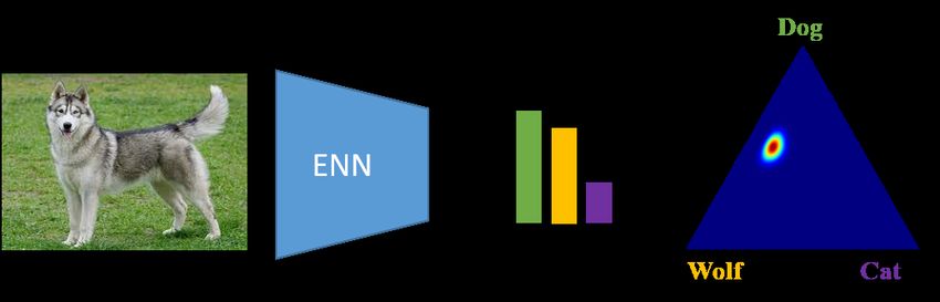
Under review as a conference paper at ICLR 2022

            (a) In-distribution image                     (b) Outlier with same class confusion
    MCP = 0.50 , entropy = 0.97, KLoS = 97.85          MCP = 0.50 , entropy = 0.97, KLoS = 104.71

Figure 1: Limitations of first-order uncertainty measures and their handling with KLoS. (a) An
in-distribution image with conflicting evidence between dog and wolf. (b) An outlier with same class
confusion but a lower amount of evidence. An evidential neural network (ENN) outputs class-wise
evidence information as concentration parameters of a Dirichlet density (visualized on the simplex)
over 3-class distributions. Although this density is flatter for the second input, the predictive entropy
and MCP, only based on first-order statistics, are equal for both inputs. In contrast, the proposed
measure, KLoS, captures both class confusion and lack of evidence, hence correctly reflecting the
larger uncertainty for the latter sample.

shown in Fig. 1: the resulting measures are invariant to the spread of the distribution, whereas un-
certainty caused by class confusion and lack of evidence should be cumulative, a property naturally
fulfilled by the predictive variance in Bayesian regression (Murphy, 2012).
Existing OOD detection methods with evidential models (Malinin
& Gales, 2018; 2019; Nandy et al., 2020) use second-order un-
certainty measures assuming that the Dirichlet distribution spread
is larger for OOD than for in-distribution (ID) samples, e.g., pre-
cision α0 or mutual information. They also rely on using auxil-
iary OOD data during training to enforce higher distribution spread
on OOD inputs. However, this assumption is not always fulfilled
in absence of OOD training data, as noted by Charpentier et al.
(2020); Sensoy et al. (2020). As shown in Fig. 2 for a model
trained on CIFAR-10, α0 values largely overlap between IDs and          Figure 2: Precision densities
OODs when no OOD training data is used, limiting the effective-         for ID (CIFAR-10) and OOD
ness of existing second-order uncertainty measures. Consequently,       (TinyImageNet) samples when
neither current first-order nor second-order uncertainty measures       no OOD training data is used.
appear to be suited for open-world settings.
Contributions. In this paper, we introduce KLoS, a measure that accounts for both in-distribution
and out-of-distribution sources of uncertainty and that is effective even without having access to
auxiliary OOD data at train time. KLoS computes the Kullback–Leibler (KL) divergence between
model’s predicted Dirichlet distribution and a specifically designed class-wise prototype Dirichlet
distribution. By leveraging the second-order uncertainty representation that evidential models pro-
vide, KLoS captures both class confusion and lack of evidence in a single score. Prototype distri-
butions are designed with concentration parameters shared with in-distribution training data, which
enables to detect OOD samples without assuming any restrictive behavior, e.g., having low preci-
sion α0 . KLoS naturally reflects the training objective used in evidential models and we propose to
learn an auxiliary model, named KLoSNet, to regress the values of a refined objective for training
samples and to improve uncertainty estimation. To assess the quality of uncertainty estimates in
open-world recognition, we design the new task of simultaneous detection of misclassifications and
OOD samples. Extensive experiments show the benefits of KLoSNet on various image datasets and
model architectures. In presence of OOD training data, we also found that our proposed measure is
more robust to the choice of OOD samples while previous measures may perform poorly. Finally,
we show that KLoS can be successfully combined with ensembling to improve performance.

2   C APTURING I N -D ISTRIBUTION AND OOD U NCERTAINTIES

Section 2.2 presents our measure to capture class confusion and lack of evidence with evidential
models. We propose a confidence learning approach to enhance in-distribution uncertainty estima-
tion in Section 2.3. Beforehand, we review evidential models and their learning in Section 2.1 to put
in perspective the benefits of the proposed approach.

                                                   2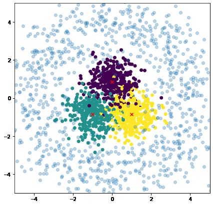
Under review as a conference paper at ICLR 2022

2.1      BACKGROUND : E VIDENTIAL N EURAL N ETWORKS

Let us consider a training dataset D of N i.i.d. samples x with label y ∈ J1, CK drawn from an un-
known joint distribution p(x, y). Bayesian models and ensembling methods approximate the poste-
rior predictive distribution P (y = c|x∗ , D) by marginalizing over the network’s parameters thanks
to sampling. But this comes at the cost of multiple forward passes. Evidential Neural Networks
(ENNs) propose instead to model explicitly the posterior distribution over categorical probabilities
p(π|x, y) by a variational Dirichlet distribution,
                                                                      C
                                                    Γ(α0 (x, θ))     Y
                                                                         πcαc (x,θ)−1 ,

                  qθ (π|x) = Dir π|α(x, θ) = QC                                                  (1)
                                                   c=1 Γ(α c (x, θ)) c=1

whose concentration parameters α(x, θ) = exp f (x, θ) are output by a network f with parameters
                                              PC
θ; Γ is the Gamma function and α0 (x, θ) = c=1 αc (x, θ). Precision α0 controls the sharpness of
the density with more mass concentrating around the mean as α0 grows. By conjugate property, the
                                                                                           fc (x∗ ,θ)
predictive distribution for a new point x∗ is P (y = c|x∗ , D) ≈ Eqθ (π|x∗ ) [πc ] = PCexpexp  fk (x∗ ,θ)
                                                                                                          ,
                                                                                      k=1
which is the usual output of a network f with softmax activation.
The concentration parameters α can be interpreted as pseudo-counts representing the amount of
evidence in each class. For instance, in Fig. 1a, the α’s output by the ENN indicates that the image
is almost equally likely to be classified as wolf or as dog. More interestingly, it also distinguishes
this in-distribution images from the OOD sample in Fig. 1b via the total amount of evidence α0 .
Training Objective. The ENN training is formulated as a variational approximation to minimize
the KL divergence between qθ (π|x) and the true posterior distribution p(π|x, y):

       Lvar (θ; D) = E(x,y)∼p(x,y) KL qθ (π|x) k p(π|x, y)                                (2)
                     1    X
                   ∝            − ψ(αy (x, θ))−ψ(α0 (x, θ)) + KL qθ (π|x) k p(π|x) ,      (3)
                     N
                             (x,y)∈D

where ψ is the digamma function. Following Joo et al. (2020), we use the non-informative uniform
prior p(π|x) = Dir π|1 , where 1 is the all-one vector, and weigh the KL divergence term with
λ > 01 :
                         1 X
          Lvar (θ; D) =            − ψ(αy ) − ψ(α0 ) + λKL Dir(π|α) k Dir(π|1) .               (4)
                        N
                                 (x,y)∈D

In particular, minimizing loss Eq. (4) enforce training sample’s precision α0 to remain close to
C + λ−1 value (Malinin & Gales, 2019).

2.2      A K ULLBACK –L EIBLER D IVERGENCE M EASURE ON THE S IMPLEX

By explicitly learning a distribution of the categorical probabilities π, evidential models provide a
second-order uncertainty representation where the expectation of the Dirichlet distribution relates
to class confusion and its spread to the amount of evidence. While originally used to measure the
total uncertainty, the predictive entropy H[y|x, θ] and the maximum class probability MCP(x, θ) =
maxc P (y = c|x, θ) only account for the position on the simplex. These measures are invariant
to the dispersion of the Dirichlet distribution that generates the categorical probabilities. This can
be problematic, as illustrated in Fig. 1. To capture uncertainties due to class confusion and lack of
evidence, an effective measure should account for the sharpness of the Dirichlet distribution and its
location on the simplex.
We introduce a novel measure, named KLoS for “KL on Simplex”, that computes the KL divergence
between the model’s output and a class-wise prototype Dirichlet distribution with concentrations γŷ
focused on the predicted class ŷ:

                         KLoS(x) , KL Dir π|α(x, θ) k Dir π|γŷ ,                                (5)
where α(x, θ) = exp f (x, θ) are model’s output and γŷ = (1, . . . , 1, τ, 1, . . . , 1) are the uniform
concentration parameters except for the predicted class with τ = 1 + λ−1 .
   1
       For conciseness, we denote αc = αc (x, θ), ∀c hereafter.

                                                        3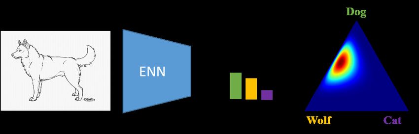
Under review as a conference paper at ICLR 2022
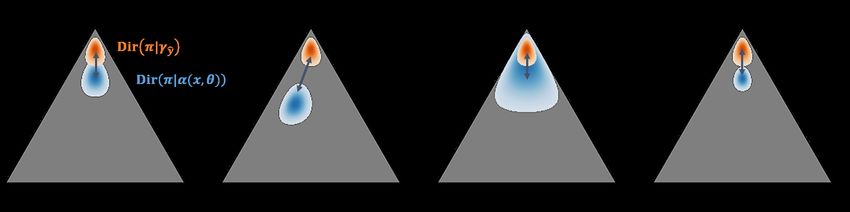
Figure 3: KLoS and KLoS∗ on the probability simplex. Given the input sample, the blue region
represents the distribution predicted by the evidential model and the orange region represents the
prototype Dirichlet distribution with parameters γŷ = (1, · · · , 1, τ, 1, . . . , 1) focused on the pre-
dicted class ŷ. Illustration of the behavior of KLoS in absence of uncertainty (a), in case of class
confusion (b) and in case of a different amount of evidence, either lower (c) or higher (d).
The lower KLoS is, the more certain the prediction is. Correct predictions will have Dirich-
let distributions similar to the prototype Dirichlet distribution γŷ and will thus be associated
with a low uncertainty score (Fig. 3a). Samples with high class confusion will present an ex-
pected probability distributions closer to simplex’s center than the expected class-wise prototype
p∗ŷ = ( K−1+τ
1 τ
, · · · , K−1+τ 1
, . . . , K−1+τ ), resulting in a higher KLoS score (Fig. 3b). Similarly,
KLoS also penalizes samples having a different precision α0 than the precision α0∗ = τ +C−1 of
the prototype γŷ . Samples with smaller (Fig. 3c) and higher (Fig. 3d) amount of evidence than α0∗
receive a larger KLoS score.
Effective measure without OOD training data. Since in-distribution samples are enforced to have
precision close to α0∗ during training, the class-wise prototypes are fine estimates of the concentra-
tion parameters of training data for each class. Hence, KLoS is a divergence-based metric, which
only needs in-distribution data during training to compute its prototypes. This behavior is illustrated
in Section 4.1. The proposed measure will be effective to detect various types of OOD samples
whose precision is far from α0∗ . In contrast, second-order uncertainty measures, e.g., mutual infor-
mation, assume that OOD samples have smaller α0 , a property difficult to fulfill for models trained
only with in-distribution samples (see Fig. 2). In Section 4.3, we explore more in-depth the impact
of the choice of OOD training data on the actual α0 values for OOD samples.
By approximating the digamma function ψ (see Appendix B), KLoS can also be decomposed as:
αŷ 1 1
KLoS(x) ≈ −(τ − 1) log + − (τ − 1)( − ) + KL Dir(π|α) k Dir(π|1) . (6)
α0 2α0 2αŷ
The first term is the standard log-likelihood and relates only to expected probabilities, hence to the
class confusion. The ratio αŷ /α0 makes it invariant to any scaling of the concentration parameters
vector α. The other terms take into account the spread of the distribution by measuring how close
α0 is to (τ +C−1), and measure the amount of evidence.
2.3 I MPROVING U NCERTAINTY E STIMATION WITH C ONFIDENCE L EARNING
When the model misclassifies an example, i.e., the predicted class ŷ differs
from the ground truth y, KLoS measures the distance between the ENN’s
output and the wrongly estimated posterior p(π|x, ŷ). This may result in an
arbitrarily high confidence / low KL divergence value. Measuring instead the
distance to the true posterior distribution p(π|x, y) (Fig. 4) would more likely
yield a greater value, reflecting the fact that the classifier made an error. Thus,
a better measure for misclassification detection would be: Figure 4: KLoS∗
KLoS∗ (x, y) , KL Dir π|α(x, θ) k Dir π|γy ,
(7)
−1
where γy corresponds to the uniform concentrations except for the true class y with τ = 1 + λ .
∗
Connecting KLoS with Evidential Training Objective. Choosing such value for τ results in
KLoS∗ matching the objective function in Eq. (4). This means that KLoS∗ is explicitly minimized
by the evidential model during training for in-distribution samples. By mimicking the evidential
4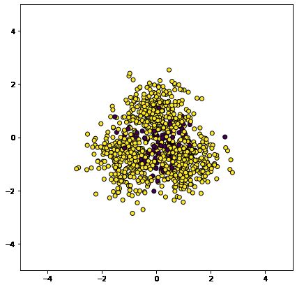
Under review as a conference paper at ICLR 2022

training objective, we reflect the fact that the model is confident about its prediction if KLoS∗ is close
to zero. In addition, minimizing the KL divergence between the variational distribution qθ (π|x)
and the posterior p(π|x, y) is equivalent to maximizing the evidence lower bound (ELBO). Hence,
a small KLoS∗ value corresponds to a high ELBO, which is coherent with the common assumption
in variational inference that higher ELBO corresponds to “better” models (Gal, 2016).
Obviously, the true class of an output is not available when estimating confidence on test samples.
We propose to learn KLoS∗ by introducing an auxiliary confidence neural network, KLoSNet, with
parameters ω, which outputs a confidence prediction C(x, ω). KLoSNet consists of a small decoder,
composed of several dense layers attached to the penultimate layer of the original classification
network. During training, we seek ω such that C(x, ω) is close to KLoS∗ (x, y), by minimizing
                                        1 X                                   2
                    LKLoSNet (ω; D) =                C(x, ω) − KLoS∗ (x, y) .                   (8)
                                        N
                                            (x,y)∈D
KLoSNet can be further improved by endowing it with its own feature extractor. Initialized with
the encoder of the classification network, which must remain untouched for not affecting its perfor-
mance, the encoder of KLoSNet can be fine-tuned along with its regression head. This amounts to
minimizing Eq. (8) w.r.t. to both sets of parameters.
The training set for confidence learning is the one used for classification training. In the experiments,
we observe a slight performance drop when using a validation set instead. Indeed, when dealing
with models with high predictive performance and small validation sets, we end up with fewer
misclassification examples than in the train set. At test time, we now directly use KLoSNet’s scalar
output C(x, ω 0 ) as our uncertainty estimate. As previously, the lower the output value, the more
confident the prediction.

3    R ELATED W ORK
Misclassification Detection. Several works (Jiang et al., 2018; Corbière et al., 2019; Moon et al.,
2020) aim to improve the standard MCP baseline (Hendrycks & Gimpel, 2017) in misclassification
detection with NNs. In particular, Corbière et al. (2019) design an auxiliary NN to predict a con-
fidence criterion on training points. We adapt their high-level idea for evidential models to tackle
jointly the detection of misclassified in-distribution samples and of OOD samples. With evidential
models, Shi et al. (2020) use dissonance in their active learning framework. In contrast to other
second-uncertainty measures, dissonance relates to class confusion, but does not acknowledge for
the amount of evidence.
Out-of-Distribution Detection. Bayesian neural networks (Neal, 1996) and ensembling (Laksh-
minarayanan et al., 2017) offer a principled approach for uncertainty estimation in which a second-
order measure can be derived by measuring the dispersion between individual probabilities vectors.
But this comes at the expense of an increased computational cost. Evidential models emulate an en-
semble of models using a single network, but usually require OOD samples during training (Malinin
& Gales, 2018; 2019; Nandy et al., 2020), which may be unrealistic in many applications. KLoS
alleviates this constraint and remains effective without OOD in training. Another range of methods
proposes to improve OOD detection on any pre-trained model. ODIN (Liang et al., 2018) mitigates
over-confidence by post-processing logits with temperature scaling and by adding inverse adver-
sarial perturbations. Lee et al. (2018) proposes a confidence score based on the class-conditional
Mahalanobis distance, with the assumption of tied covariance. Although effective, both approaches
need OOD data to tune hyperparameters, which might not generalize to other OOD datasets (Shafaei
et al., 2019). Finally, Liu et al. (2020) interpret a pre-trained NN as an energy-based model and
compute the energy score to detect OOD samples. Interestingly, this score corresponds to the log
precision log α0 , which is similar to the EPKL measure Malinin & Gales (2019) used in ENNs.

4    E XPERIMENTS
In this section, we assess our method against existing baseline uncertainty measures on synthetic data
and we conduct extensive experiments across various image datasets, architectures and settings.
Experimental Setup. Uncertainty measures are derived from an evidential model (Eq. (4)) with
λ = 10−2 as in (Joo et al., 2020; Malinin & Gales, 2019), except for second-order metrics where

                                                    5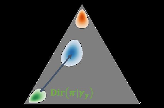
Under review as a conference paper at ICLR 2022

  (a) Toy dataset   (b) Corr./Err.    (c) Entropy       (d) Mut. Inf.   (e) Mahalanobis   (f) KLoS

Figure 5: Comparison of various uncertainty measures for a given evidential classifier on a toy
dataset. (a) Training samples from 3 input Gaussian distributions with large overlap (hence class
confusion) and OOD test samples (blue); (b) Correct (yellow) and erroneous (red) class predictions
on in-domain test samples; (c-f) Visualisation of different uncertainty measures derived from the
evidential model trained on the toy dataset. Yellow (resp. purple) indicates high (resp. low) certainty.

we found that setting λ = 10−3 improves performance. We rely on the learned classifier to train our
auxiliary confidence model KLoSNet, using the same training set and following loss Eq. (8). All
details about architectures, training algorithms and datasets are available in Appendix C.
Baselines. We evaluate our approach against: first-order uncertainty metrics (Maximum Class prob-
ability (MCP) and predictive entropy (Entropy)), second-order metrics (mutual information (Mut.
Inf.) and dissonance), post-training methods for OOD detection (ODIN and Mahalanobis) and for
misclassification detection (ConfidNet). Except in Section 4.3, we consider setups where no OOD
data is available for training. Consequently, the results reported for ODIN and Mahalanobis are
obtained without adversarial perturbations, which is also the best configuration for the considered
tasks. We indeed show in Appendix D.6 that these perturbations degrade misclassification detection.

4.1   S YNTHETIC E XPERIMENT

We analyse the behavior of the KLoS measure and the limitations of existing first- and second-order
uncertainty metrics on a 2D synthetic dataset composed of three Gaussian-distributed classes with
equidistant means and identical isotropic variance (Fig. 5). This constitutes a scenario with high
first-order uncertainty due to class overlap. OOD samples are drawn from a ring around the in-
distribution dataset and are only used for evaluation. Fig. 5c shows that Entropy correctly assigns
large uncertainty along decision boundaries, which is convenient to detect misclassifications, but
yields low uncertainty for points far from the distribution. Mut. Inf. (Fig. 5d) have the opposite
behavior than desired by decreasing when moving away from the training data. This is due to
the linear nature of the toy dataset where models assign higher concentration parameters far from
decision boundaries, hence smaller spread on the simplex, as also noted in (Charpentier et al., 2020).
Additionally, Mut. Inf. does not reflect the uncertainty caused by class confusion along decision
boundaries. Neither Entropy nor Mut. Inf. is suitable to detect OOD samples in this synthetic
experiment. In contrast, KLoS allows discriminating both misclassifications and OOD samples from
correct predictions as uncertainty increases far from in-distribution samples for each class (Fig. 5f).
KLoS measures a distance between the model’s output and a class-wise prototype distribution. Here,
we can observe that it acts as a divergence-based measure for each class.
We extend the comparison to include Mahalanobis (Fig. 5e), which is a distance-based measure by
assuming Gaussian class conditionals on latent representations, here in the input space. However,
Mahalanobis does not discriminate points close to the decision boundaries from points with a similar
distance to the origin. Hence, it may be less suited to detect misclassifications than KLoS. Addi-
tionally, KLoS does not assume Gaussian distributions in the latent space nor tied covariance, which
may be a strong assumption when dealing with high-dimension latent space. In Appendix D.1, a
complementary quantitative evaluation on this toy problem confirms our findings regarding the inad-
equacy of first-order uncertainty measures such as MCP and Entropy, and the improvement provided
by KLoS over Mahalanobis on misclassification detection.

4.2   C OMPARATIVE E XPERIMENTS

The task of detecting both in-distribution misclassifications and OOD samples gives the opportunity
to jointly evaluate in-distribution and out-of-distribution uncertainty representations of a method.
In this binary classification problem, correct predictions are considered as positive samples while

                                                    6
Under review as a conference paper at ICLR 2022 Table 1: Comparative experiments on CIFAR-10 and CIFAR-100. Misclassification (Mis.), out- of-distribution (OOD) and simultaneous (Mis+OOD) detection results (mean % AUROC and std. over 5 runs). Bold type indicates significantly best performance (p
Under review as a conference paper at ICLR 2022

Table 2: Impact of confidence learning. Comparison of detection performances between KLoS
and KLoSNet for CIFAR-10 and CIFAR-100 experiments with VGG-16 architecture.

                                             LSUN               TinyImageNet                 STL-10
              Method       Mis.        OOD      Mis+OOD        OOD     Mis+OOD         OOD      Mis+OOD
 CIFAR-10     KLoS       92.1 ±0.3   86.5 ±0.3   91.2 ±0.2   85.4 ±0.3   90.4 ±0.2   64.1 ±0.3   79.6 ±0.3
  VGG-16      KLoSNet    92.5 ±0.6   87.6 ±0.9   91.7 ±0.9   86.6 ±0.9   91.2 ±0.8   67.7 ±1.4   81.8 ±0.9
 CIFAR-100    KLoS       85.4 ±0.2   65.1 ±1.1   81.3 ±0.6   74.5 ±0.4   85.4 ±0.4   72.7 ±0.3   84.8 ±0.4
  VGG-16      KLoSNet    86.7 ±0.4   68.4 ±1.1   83.0 ±0.6   76.4 ±0.4   86.4 ±0.4   75.0 ±0.5   86.0 ±0.4

Figure 6: Effect of OOD training data on precision α0 . Den-
sity plots for CIFAR-10/TinyImageNet benchmark: (a,b) with in-            Figure 7: Impact of the over-
appropriate OOD samples (SVHN, LSUN); (c) with close OOD                  sampling factor κ (CIFAR-
samples (CIFAR-100).                                                      10/TinyImageNet).

logits are small due to regularization in the evidential training objective. Mut. Inf. and other spread-
based second-order uncertainty measures (see Appendix D.2) fall short to detect correctly OOD.
Indeed, for settings where OOD training data is not available, there is no guarantee that every OOD
sample will result in lower predicted concentration parameters as previously shown by the density
plot of precision α0 in Fig. 2. This stresses the importance of class-wise divergence-based measure.
While Mahalanobis may sometimes be slightly better than KLoSNet for OOD detection, it performs
significantly less well in misclassification detection, in line with the behavior shown in synthetic
experiments. As a result, KLoSNet appears to be the best measure in every simultaneous detection
benchmark. For instance, for CIFAR-10/STL-10 with VGG-16, KLoSNet achieves 81.8% AUROC
while the second best, Mahalanobis, scores 78.8%. We also observe that KLoSNet improves sig-
nificantly misclassification detection, even compared to dedicated methods such as ConfidNet or
second-order measures related to class confusion, e.g., dissonance. Another baseline could be to
combine two measures specialized respectively for class confusion and lack of evidence, such as
Dissonance+Mut.Inf. But it still performs less well than KLoSNet. In Appendix E, we evaluate
our approach on the task of selective classification when inputs are subject to corruptions (which
can be seen as OOD samples close to the input distribution, hence particularly challenging), and we
observe similar results.
Impact of Confidence Learning. To evaluate the effect of the uncertainty measure KLoS and
of the auxiliary confidence network KLoSNet, we report a detailed ablation study in Table 2. We
can notice that KLoSNet improves misclassification over KLoS but also OOD detection in every
benchmark. We intuit that learning to improve misclassification detection also helps to spot some
OOD inputs that share similar characteristics.
Oversampling Factor. When deploying a model in the wild, it is difficult to know beforehand the
proportions of misclassifications and OOD samples it will have to handle. We vary the oversampling
factor κ in [0.01; 100] for CIFAR10/TinyImageNet in Fig. 7 to assess the robustness of our approach.
KLoSNet consistently outperforms all other measures, with a larger gain when κ increases.
Combining KLoS with Ensembling. Aggregating predictions from an ensemble of neural net-
works not only improves generalization (Lakshminarayanan et al., 2017; Rame & Cord, 2021) but
also uncertainty estimation (Ovadia et al., 2019a). We train an ensemble of ten evidential models
on CIFAR-10 and evaluate the performance of KLoS obtained from averaged concentration param-
eters. On CIFAR-10/TinyImageNet benchmark, misclassification and OOD detection performances
are improved by respectively +1.8 points and +1.9 points, resulting in a +1.1 points gain on the
joint detection task.

                                                    8
Under review as a conference paper at ICLR 2022
(a) Mis. detection (b) OOD detection (c) Mis.+OOD detection
Figure 8: Comparative detection results with different OOD training datasets. While using
OOD samples in training improves performance in general, the gain value varies widely, sometimes
even being negative for inappropriate OOD samples e.g., SVHN. KLoS remains the best measure in
every setting. Experiment with VGG-16 architecture on CIFAR-10 dataset.
4.3 E FFECT OF T RAINING WITH O UT- OF -D ISTRIBUTION S AMPLES
Previous results demonstrate that simultaneous detection of misclassifications and OOD samples
can be significantly improved by KLoSNet. We now investigate settings where OOD samples are
available. We train an evidential model to minimize the reverse KL-divergence (Malinin & Gales,
2019) between the model output and a sharp Dirichlet distribution focused on the predictive class for
in-distribution samples, and between the model output and a uniform Dirichlet distribution for OOD
samples. This loss induces low concentration parameters for OOD data and improves second-order
uncertainty measures such as Mut. Inf
The literature on evidential models only deals with an OOD training set somewhat related to the in-
distribution dataset, e.g. CIFAR-100 for models trained on CIFAR-10. Despite semantic differences,
CIFAR-10 and CIFAR-100 images were collected the same way, which might explain the general-
isation to other OOD samples in evaluation. Contrarily, CIFAR-10 objects and SVHN street-view
numbers differ more for instance. In Fig. 8, we vary the OOD training set and compare the uncer-
tainty metrics taken from the resulting models. As expected, using CIFAR-100 as training OOD data
improves performance for every measure (MCP, Mut. Inf. and KLoS). However, the boost provided
by training with OOD samples depends highly on the chosen dataset: The performance of Mut. Inf.
decreases from 92.6% AUC with CIFAR-100 to 82.9% when switching to LSUN, and even becomes
worse with SVHN (78.5%) compared to using no OOD data (80.6%). Indeed, Fig. 6 shows that only
the CIFAR-100 dataset seems to be effective to enforce low α0 on unseen OOD samples.
We also note that KLoS outperforms or is on par with MCP and Mut. Inf. in every setting. These
results confirm the adequateness of KLoS for simultaneous detection and extend our findings to
settings where OOD data is available at train time. Most importantly, using KLoS on models with-
out OOD training data yields better detection performance than other measures taken from models
trained with inappropriate OOD samples, here being every OOD dataset other than CIFAR-100.
5 D ISCUSSION
We propose KLoSNet, an auxiliary model to estimate the uncertainty of a classifier for both in-
domain and out-of-domain inputs. Based on evidential models, KLoSNet is trained to predict the
KLoS∗ value of a prediction. By design, KLoSNet encompasses both class confusion and evidence
information, which is necessary for open-world recognition. Our experiments extensively demon-
strate its effectiveness across various architectures, datasets and configurations, and reveal its class-
wise divergence-based behavior. Many real-world applications, e.g., based on active learning or
domain adaptation, necessitate to correctly detect both sources of uncertainty. It will be interesting
to apply KLoSNet in these contexts. We also show that, far from being the panacea, using training
OOD samples depends critically on the choice of these samples for existing uncertainty measures.
KLoS, on the other hand, is more robust to this choice and can alleviate their use altogether. While
finding suitable OOD samples may be easy for some academic datasets, it may turn more problem-
atic in real-world applications, with the risk of degrading performance with an inappropriate choice.
How to build suitable OOD training sets is an important open problem to attack.
9Under review as a conference paper at ICLR 2022
6 R EPRODUCIBILITY S TATEMENT
To better understand the link between the evidential training objective and KLoS* criterion stated
in Appendix A.2, we provide a detailed derivation in Appendix A. We also elaborate on the the-
oretical decomposition of KLoS (Eq. (6)) in Appendix B. Regarding experiments reproducibility,
Appendix C describes extensively how we generate data in the synthetic experiment (Section 4.1),
the image classification datasets used to evaluate our approach including in-distribution and OOD
datasets, the implementation and the hyperparameters of the experiments shown in Section 4.2. In
particular, we took care in our experiments to perform multiple runs and present mean and std re-
sults. Giving access to the code has yet to be authorized internally, but we plan to release the code
in the future.
R EFERENCES
Abhijit Bendale and Terrance Boult. Towards open world recognition. In IEEE/CVF Conference on
Computer Vision and Pattern Recognition, 2015. 1
Bertrand Charpentier, Daniel Zügner, and Stephan Günnemann. Posterior network: Uncertainty esti-
mation without ood samples via density-based pseudo-counts. In Advances in Neural Information
Processing Systems, 2020. 2, 6, 16
Adam Coates, Andrew Ng, and Honglak Lee. An analysis of single-layer networks in unsupervised
feature learning. In Proceedings of the International Conference on Artificial Intelligence and
Statistics, 2011. 7
Charles Corbière, Nicolas Thome, Avner Bar-Hen, Matthieu Cord, and Patrick Pérez. Addressing
failure prediction by learning model confidence. In Advances in Neural Information Processing
Systems, 2019. 5
Ran El-Yaniv and Yair Wiener. On the foundations of noise-free selective classification. Journal of
Machine Learning Research, 2010. 21
Yarin Gal. Uncertainty in Deep Learning. PhD thesis, University of Cambridge, 2016. 5
Yarin Gal and Zoubin Ghahramani. Dropout as a Bayesian approximation: Representing model un-
certainty in deep learning. In Proceedings of the International Conference on Machine Learning,
2016. 1
Kaiming He, Xiangyu Zhang, Shaoqing Ren, and Jian Sun. Deep residual learning for image recog-
nition. In IEEE/CVF Conference on Computer Vision and Pattern Recognition, 2016. 7
David Heckerman, Eric Horvitz, and Bharat Nathwani. Toward normative expert systems: Part
i the pathfinder project. Methods of information in medicine, 31, 07 1992. doi: 10.1055/
s-0038-1634867. 1
Matthias Hein, Maksym Andriushchenko, and Julian Bitterwolf. Why relu networks yield high-
confidence predictions far away from the training data and how to mitigate the problem. In
IEEE/CVF Conference on Computer Vision and Pattern Recognition, 2019. 1
Dan Hendrycks and Thomas Dietterich. Benchmarking neural network robustness to common cor-
ruptions and perturbations. In Proceedings of International Conference on Learning Representa-
tions, 2019. 21
Dan Hendrycks and Kevin Gimpel. A baseline for detecting misclassified and out-of-distribution
examples in neural networks. In Proceedings of International Conference on Learning Represen-
tations, 2017. 1, 5, 7
Heinrich Jiang, Been Kim, Melody Guan, and Maya Gupta. To trust or not to trust a classifier. In
Advances in Neural Information Processing Systems, 2018. 5
Taejong Joo, Uijung Chung, and Min-Gwan Seo. Being bayesian about categorical probability. In
Proceedings of the International Conference on Machine Learning, 2020. 1, 3, 5, 13
10Under review as a conference paper at ICLR 2022
Audun Josang. Subjective Logic: A Formalism for Reasoning Under Uncertainty. Springer, 2016. 1
Pang Wei Koh, Shiori Sagawa, Henrik Marklund, Sang Michael Xie, Marvin Zhang, Akshay Bal-
subramani, Weihua Hu, Michihiro Yasunaga, Richard Lanas Phillips, Sara Beery, Jure Leskovec,
Anshul Kundaje, Emma Pierson, Sergey Levine, Chelsea Finn, and Percy Liang. Wilds: A bench-
mark of in-the-wild distribution shifts. arxiv, 2020. 21
A Krizhevsky. Learning multiple layers of features from tiny images. Master’s thesis, Department
of Computer Science, University of Toronto, 2009. 7, 16
Balaji Lakshminarayanan, Alexander Pritzel, and Charles Blundell. Simple and scalable predictive
uncertainty estimation using deep ensembles. In Advances in Neural Information Processing
Systems, 2017. 1, 5, 8
Kimin Lee, Kibok Lee, Honglak Lee, and Jinwoo Shin. A simple unified framework for detecting
out-of-distribution samples and adversarial attacks. In Advances in Neural Information Process-
ing Systems, 2018. 5, 19
Shiyu Liang, Yixuan Li, and R. Srikant. Enhancing the reliability of out-of-distribution image detec-
tion in neural networks. In Proceedings of International Conference on Learning Representations,
2018. 5, 19
Weitang Liu, Xiaoyun Wang, John Owens, and Yixuan Li. Energy-based out-of-distribution detec-
tion. In Advances in Neural Information Processing Systems, 2020. 5
Wesley J Maddox, Pavel Izmailov, Timur Garipov, Dmitry P Vetrov, and Andrew Gordon Wilson.
A simple baseline for Bayesian uncertainty in deep learning. In Advances in Neural Information
Processing Systems 32, 2019. 1
Andrey Malinin and Mark Gales. Predictive uncertainty estimation via prior networks. In Advances
in Neural Information Processing Systems, 2018. 1, 2, 5
Andrey Malinin and Mark Gales. Reverse kl-divergence training of prior networks: Improved uncer-
tainty and adversarial robustness. In Advances in Neural Information Processing Systems, 2019.
1, 2, 3, 5, 9, 16
Rowan McAllister, Yarin Gal, Alex Kendall, Mark van der Wilk, Amar Shah, Roberto Cipolla, and
Adrian Weller. Concrete problems for autonomous vehicle safety: Advantages of Bayesian deep
learning. In Proceedings of the International Joint Conference on Artificial Intelligence, 2017. 1
Jooyoung Moon, Jihyo Kim, Younghak Shin, and Sangheum Hwang. Confidence-aware learning
for deep neural networks. In Proceedings of the International Conference on Machine Learning,
2020. 5
Kevin P. Murphy. Machine learning : A Probabilistic Perspective. MIT Press, 2012. 2
Jay Nandy, Wynne Hsu, and Mong-Li Lee. Towards maximizing the representation gap between in-
domain and out-of-distribution examples. In Advances in Neural Information Processing Systems,
2020. 1, 2, 5, 16
Radford M. Neal. Bayesian Learning for Neural Networks. Springer-Verlag, 1996. 5
Yuval Netzer, Tao Wang, Adam Coates, Alessandro Bissacco, Bo Wu, and Andrew Y. Ng. Reading
digits in natural images with unsupervised feature learning. In NIPS Workshop on Deep Learning
and Unsupervised Feature Learning, 2011. 16, 18
A. Nguyen, J. Yosinski, and J. Clune. Deep neural networks are easily fooled: High confidence
predictions for unrecognizable images. In IEEE/CVF Conference on Computer Vision and Pattern
Recognition, 2015. 1
Yaniv Ovadia, Emily Fertig, Jie Ren, Zachary Nado, D. Sculley, Sebastian Nowozin, Joshua Dillon,
Balaji Lakshminarayanan, and Jasper Snoek. Can you trust your model's uncertainty? evaluating
predictive uncertainty under dataset shift. In Advances in Neural Information Processing Systems,
2019a. 8
11Under review as a conference paper at ICLR 2022
Yaniv Ovadia, Emily Fertig, Jie Ren, Zachary Nado, D. Sculley, Sebastian Nowozin, Joshua Dillon,
Balaji Lakshminarayanan, and Jasper Snoek. Can you trust your model's uncertainty? evaluating
predictive uncertainty under dataset shift. In Advances in Neural Information Processing Systems,
2019b. 1
Adam Paszke, Sam Gross, Francisco Massa, Adam Lerer, James Bradbury, Gregory Chanan, Trevor
Killeen, Zeming Lin, Natalia Gimelshein, Luca Antiga, Alban Desmaison, Andreas Kopf, Edward
Yang, Zachary DeVito, Martin Raison, Alykhan Tejani, Sasank Chilamkurthy, Benoit Steiner,
Lu Fang, Junjie Bai, and Soumith Chintala. PyTorch: An imperative style, high-performance
deep learning library. In Advances in Neural Information Processing Systems, 2019. 16
Alexandre Rame and Matthieu Cord. Dice: Diversity in deep ensembles via conditional redundancy
adversarial estimation. In International Conference on Learning Representations, 2021. 8
Jie Ren, Stanislav Fort, Jeremiah Liu, Abhijit Guha Roy, Shreyas Padhy, and Balaji Lakshmi-
narayanan. A simple fix to mahalanobis distance for improving near-ood detection, 2021. 19
Murat Sensoy, Lance Kaplan, and Melih Kandemir. Evidential deep learning to quantify classifica-
tion uncertainty. In Advances in Neural Information Processing Systems, 2018. 1
Murat Sensoy, Lance Kaplan, Federico Cerutti, and Maryam Saleki. Uncertainty-aware deep classi-
fiers using generative models. In Proceedings of the Thirty-Fourth AAAI Conference on Artificial
Intelligence, 2020. 2
Alireza Shafaei, Mark Schmidt, and James J. Little. A less biased evaluation of out-of-distribution
sample detectors. In BMVC, 2019. 5
W. Shi, Xujiang Zhao, Feng Chen, and Qi Yu. Multifaceted uncertainty estimation for label-efficient
deep learning. In Advances in Neural Information Processing Systems, 2020. 1, 5
Karen Simonyan and Andrew Zisserman. Very deep convolutional networks for large-scale image
recognition. In Proceedings of the International Conference on Learning Representations, 2015.
7, 16
Fisher Yu, Yinda Zhang, Shuran Song, Ari Seff, and Jianxiong Xiao. LSUN: Construction
of a large-scale image dataset using deep learning with humans in the loop. arXiv preprint
arXiv:1506.03365, 2015. 7, 16
12Under review as a conference paper at ICLR 2022
A L INK BETWEEN KL O S* AND E VIDENTIAL T RAINING O BJECTIVE
In this section, we detail the connection between KLoS* and the evidential training objective. For
conciseness, we denote αc = αc (x, θ), ∀c ∈ J0, CK hereafter.
A.1 D ERIVING THE E VIDENTIAL T RAINING O BJECTIVE
We first show the equivalence between Eq. (2) and Eq. (4). Starting from Eq. (2),
Lvar (θ; D) = E(x,y)∼p(x,y) KL qθ (π|x) k p(π|x, y) (9)
Z
1 X h qθ (π|x) i
= qθ (π|x) log (10)
N p(π|x, y)
(x,y)∈D
Z
1 X h qθ (π|x)p(y|x) i
= qθ (π|x) log (11)
N p(y|π, x)p(π|x)
(x,y)∈D
1 X h i
= Eqθ (π|x) − log p(y|π, x) + KL qθ (π|x) k p(π|x) + log p(y|x) ,
N
(x,y)∈D
(12)
where N = card(D). As the log-likelihood log p(y|x) does not depend on parameters θ,
1 X h i
min Lvar (θ; D) = min Eqθ (π|x) − log p(y|π, x) + KL qθ (π|x) k p(π|x) . (13)
θ θ N
(x,y)∈D
the reverse cross-entropy term amounts to Eπ∼qθ (π|x) − log p(y|π, x) =
For a sample (x, y),
− ψ(αy )−ψ(α0 ) where ψ is the digamma function. Hence, we recover Eq.(3) of the main paper:
1 X
min Lvar (θ; D) = − ψ(αy )−ψ(α0 ) + KL(qθ (π|x) k p(π|x)). (14)
θ N
(x,y)∈D
Considering that most of the training inputs x are associated with only one observation y in D, we
should choose small concentrations parameters β for the prior p(π|x) = Dir(π|β) to prevent the
resulting posterior distribution p(π|x) = Dir(π|β1 , ..., βy + 1, ..., βC ) from being dominated by
the prior. However, this causes exploding gradients in the small-value regimes due to the digamma
function, e.g. ψ 0 (0.01) > 10−4 .
To stabilize the optimization, we follow Joo et al. (2020) and use the non-informative uniform prior
distribution p(π|x) = Dir π|1 where 1 is the all-one vector, and we weight the KL-divergence
term with λ > 0:
1 X
Lλvar (θ; D) =
− ψ(αy ) − ψ(α0 ) + λKL Dir(π|α(x, θ)) k Dir(π|1) . (15)
N
(x,y)∈D
While Lλvar (θ; D) slightly differs from Lvar (θ; D), both functions lead to the same optima. Indeed,
by considering their gradient, we can show that a local optimum of Lvar (θ; D) is achieved for a
sample x when α∗ = (β1 , ..., βy + 1, ..., βC ) and a local optimum of Lλvar (θ; D) is α• = (1, ..., 1 +
1/λ, ..., 1). Hence, their respective ratio between each element is equal:
αi∗ αi•
∀i, j ∈ J1, CK, = . (16)
αj∗ αj•
A.2 L INK WITH KL O S*
Let us remind the definition of KLoS* as a KL divergence between the model’s output and a class-
wise prototype Dirichlet distribution with concentrations γŷ focused on the true class y:
KLoS∗ (x, y) , KL Dir π|α(x, θ) k Dir π|γy ,
(17)
13Under review as a conference paper at ICLR 2022
where α(x, θ) = exp f (x, θ) is the model’s output and γy = (1, . . . , 1, τ, 1, . . . , 1) the vector of
uniform concentration parameters except for the true class with τ = 1/λ + 1.
The KL divergence between two Dirichlet distributions can be obtained in closed form and KLoS*
can be calculated as:
KLoS∗ (x, y) = KL Dir π|α k Dir π|γy
(18)
C
X
= log Γ(α0 ) − log Γ(C − 1 + 1/λ) + log Γ(1 + 1/λ) − log Γ(αc )
c=1
X
+ αc − 1 ψ(αc ) − ψ(α0 ) + αy − (1 + 1/λ) ψ(αy ) − ψ(α0 ) (19)
c6=y
On the other hand,
the KL-divergence between the model’s output and an uniform Dirichlet distri-
bution Dir π|1 reads:
C C
X X
KL Dir π|α k Dir π|1 = log Γ(α0 )−log Γ(C)− log Γ(αc )+ αc −1 ψ(αc )−ψ(α0 ) .
c=1 c=1
(20)
Hence, KLoS* can be written as:
1
KLoS∗ (x, y) = −
ψ(αy ) − ψ(α0 ) + KL Dir(π|α) k Dir(π|1)
λ
+ log Γ(1 + 1/λ) − log Γ(C − 1 + 1/λ) − log Γ(C) . (21)
Let us decompose Lλvar (θ; D) = N1 (x,y)∈D lvar λ
(x, y, θ). We retrieve that KLoS∗ (x) ∝
P
λ
lvar (x, y, θ) + r where r = − log Γ(1 + 1/λ) − log Γ(C − 1 + 1/λ) − log Γ(C) does not depend
on the model parameters θ.
In summary, minimizing the evidential training objective Lλvar (θ; D) is equivalent to minimizing the
KLoS∗ value of each training point x.
B D ECOMPOSITION OF KL O S
This section provides details of the derivation of Eq. (6). Let us remind the definition of KLoS as
a KL divergence between the model’s output and a class-wise prototype Dirichlet distribution with
concentrations γŷ focused on the predicted class ŷ:
KLoS(x) , KL Dir π|α(x, θ) k Dir π|γŷ , (22)
where α(x, θ) = exp f (x, θ) is the model’s output and γŷ = (1, ..., τ, ..., 1) the vector of uniform
concentration parameters except for the predicted class with τ > 1. For conciseness, we denote
αc = αc (x, θ), ∀c ∈ J0, CK hereafter.
Similar to the derivation done in Appendix A.2, KLoS can be derived as:
KLoS(x) = −(τ − 1) ψ(αŷ ) − ψ(α0 ) + KL Dir(π|α) k Dir(π|1) , (23)
where 1 is the all-one vector.
1
By considering the asymptotic series approximation to the digamma function, ψ(x) = log x − 2x +
1
O( x2 ), the previous expression can be approximated by:
αŷ 1 1
KLoS(x) ≈ −(τ − 1) log( ) + − (τ − 1)( − )) + KL Dir(π|α) k Dir(π|1) . (24)
α0 2α0 2αŷ
To gain further intuition about the decomposition, we provide Method Mis. (↑) OOD (↑)
illustrations of the first term (negative log-likelihood, NLL)
NLL term 80.2 ±1.1 15.9 ±0.7
and the second term in Fig. 9, similar to those shown in Fig. 3 Second term 48.2 ±4.3 98.4 ±0.1
of the paper. We also present quantitative results in Table 3. KLoS 79.4 ±1.2 98.8 ±0.3
We observe that the NLL term, which is equivalent to MCP
Table 3: Results of KLoS decompo-
14 sition on synth. data.Under review as a conference paper at ICLR 2022
measure, helps to detect misclassifications while the second
term denotes increasing uncertainty as we move either far
away from training data. Hence, by using either the NLL term
or the second term, one could distinguish the source of uncertainty if needed.
In particular, we can show that the second term reaches its minimum for α0 = τ + C − 1 thanks to
the following lemma.
(a) KLoS (b) NLL term (c) Second term
Figure 9: Visualisation of the different terms of KLoS, derived from the evidential model trained on
the same toy dataset than in the main paper.
Lemma B.1. A local minimum of g : α0 → −(τ − 1)( 2α1 0 − 2α1 ŷ )) + KL Dir(π|α) k Dir(π|1)
is reached for α0 = τ + C − 1.
Proof. Let us denote µ ∈ RC such as ∀c, αc = µc · α0 . By the definition of the KL divergence
between two Dirichlet distributions, g reads:
C C
1 − µŷ 1 X X
g : α0 → −(τ − 1) + log Γ(α0 ) − log Γ(µc α0 ) + (µc α0 − 1) ψ(µc α0 ) − ψ(α0 ) .
2µŷ α0 c=1 c=1
(25)
By taking the derivative:
C C
d 1 − µŷ 1 X X
g(α0 ) = (τ − 1) + ψ(α0 ) − µc ψ(µc α0 ) + µc ψ(µc α0 ) − ψ(α0 )
dα0 2µŷ α02 c=1 c=1
C
X
(µc α0 − 1) µc ψ (1) (µc α0 ) − ψ (1) (α0 ) , (26)
+
c=1
d
PC
where ψ (1) (x) = dx ψ(x) is the trigamma function. As c=1 µc = 1, the previous equation
simplifies to:
C
d 1 − µŷ 1 X
(µc α0 − 1) µc ψ (1) (µc α0 ) − ψ (1) (α0 ) .
g(α0 ) = (τ − 1) 2 + (27)
dα0 2µŷ α0 c=1
1 1
We consider the asymptotic series approximation to the trigamma function ψ (1) (x) = x + 2x2 +
O( x12 ). Given this approximation, the derivative reads:
C
d 1 − µŷ 1 X 1 1 1 1
g(α0 ) ≈ (τ − 1) 2 + (µc α0 − 1) µc ( + 2 2 −( − 2 (28)
dα0 2µŷ α0 c=1 µc α0 2µc α0 α0 2α0
C
1 − µŷ 1 X 1 − µc 1
= (τ − 1) 2 + (µc α0 − 1) . (29)
2µŷ α0 c=1 2µc α02
The derivative vanishes when ∀c 6= ŷ, µc α0 = 1 and µŷ α0 = τ , hence a local minimum of g is
reached for α0 = τ + C − 1.
15Under review as a conference paper at ICLR 2022
C E XPERIMENTAL S ETUP
In this section, we provide comprehensive details about the datasets, the implementation and the
hyperparameters of the experiments shown in Section 4 of the main paper.
Synthetic Data. The training dataset (Fig. 3 of the paper) consists of 1,000 samples (x, y) from a
distribution p(x, y) over R2 × {1, 2, 3} defined as:
1
p(x = x, y = y) = N (x = x|µy , σ 2 I2×2 ), (30)
3
√ √ √
where µ1 = (0, 3/2), µ2 = (−1, − 3/2) , µ3 = (1, − 3/2) and σ = 4. The marginal distribu-
tion of x is a Gaussian mixture with three equally weighted components having equidistant centers
and equal spherical covariance matrices. The test dataset consists of 1,000 other samples from this
distribution. Finally, we construct an out-of-distribution (OOD) dataset following Malinin & Gales
(2019), by sampling 100 points in R2 such that they form a ‘ring’ with large noise around the train-
ing points. Some OOD samples will be close to the in-distribution while others will be very far (see
Fig. 3 of the paper). The number of OOD samples has been chosen so that it amounts approximately
to the number of test points misclassified by the classifier. The classification is performed by a
simple logistic regression.
A set of five models is trained for 200 epochs using the evidential training objective (Eq. 6 of the
paper) with regularization parameter λ = 5e-2 and Adam optimizer with learning rate 0.02. Un-
certainty metrics – MCP, Entropy, Mut. Inf., Malahanobis and KLoS – are computed from these
models.
Image Classification Datasets. In Sections 4.2 and 4.3 of the main paper, the experiments are
conducted using CIFAR-10 and CIFAR-100 datasets Krizhevsky (2009). They consist in 32 × 32
natural images featuring 10 object classes for CIFAR-10 and 100 classes for CIFAR-100. Both
datasets are composed with 50,000 training samples and 10,000 test samples. We further randomly
split the training set to create a validation set of 10,000 images.
OOD datasets are TinyImageNet2 – a subset of ImageNet (10,000 test images with 200 classes) –,
LSUN Yu et al. (2015) – a scene classification dataset (10,000 test images of 10 scenes) –, STL-10
– a dataset similar to CIFAR-10 but with different classes, and SVHN Netzer et al. (2011) – an RGB
dataset of 28×28 house-number images (73,257 training and 26,032 test images with 10 digits) –.
We downsample each image of TinyImageNet, LSUN and STL-10 to size 32×32.
Training Details. We implemented in PyTorch Paszke et al. (2019) a VGG-16 architecture Si-
monyan & Zisserman (2015) in line with the previous works of Charpentier et al. (2020); Malinin
& Gales (2019); Nandy et al. (2020), with fully-connected layers reduced to 512 units. Models are
trained for 200 epochs with a batch size of 128 images, using a stochastic gradient descent with Nes-
terov momentum of 0.9 and weight decay 5e-4. The learning rate is initialized at 0.1 and reduced
by a factor of 10 at 50% and 75% of the training progress. Images are randomly horizontally flipped
and shifted by ±4 pixels as a form of data augmentation.
Balancing Misclassification and OOD Detection. Most neural
CIFAR-10 CIFAR-100
networks used in our experiments tend to overfit, which leaves very
Train 99.0 ±0.1 91.2 ±0.2
few training errors available. We provide accuracies on training, val- Val 93.6 ±0.1 70.6 ±0.3
idation and test sets in Table 4. With such high predictive perfor- Test 93.0 ±0.3 70.1 ±0.4
mances, the number of misclassifications is usually lower than the
number of OOD samples (∼10,000). Hence, the oversampling ap- Table 4: Mean accuracies
proach proposed in the paper helps to better balance misclassifica- (%) and std. over five runs.
tion detection performances and OOD detection performances in the
reported metrics.
KLoSNet. We start from the pre-trained evidential model described above. As detailed in Section
3.2 of the main paper, KLoSNet consists of a small decoder attached to the penultimate layer of
2
https://tiny-imagenet.herokuapp.com/
16Under review as a conference paper at ICLR 2022
Table 6: Other baselines results on comparative experiments on CIFAR-10 and CIFAR-100.
Bold type indicates significantly best performance (p1000), one may encounter some issues when training KLoSNet.
Consequently, we apply a sigmoid function, σ(x) = 1+e1−x , after computing the KL-divergence
between the NN’s output and γy . To prevent over-fitting, training is stopped when validation AUC
metric for misclassification detection starts decreasing. Then, a second training step is performed
by initializing new encoder E 0 such that θE 0 = θE initially and by optimizing weights (θE 0 , ω) for
30 epochs with Adam optimizer with learning rate 1e-6. We stop training once again based on the
validation AUC metric.
D A DDITIONAL R ESULTS
D.1 D ETAILED R ESULTS FOR S YNTHETIC E XPERIMENTS
We detail in Table 5 the quantitative results for Method Mis. (↑) OOD (↑) Mis+OOD (↑)
the task of simultaneous detection of misclas- MCP 80.2 ±1.1 15.9 ±0.7 48.6 ±1.9
sifications and of OOD samples for the syn- Entropy 78.4 ±1.5 11.0 ±0.3 45.7 ±1.0
thetic experiment presented in Section 4.1 of Mut. Inf. 75.0 ±2.3 2.2 ±0.2 38.8 ±1.2
the paper. First-order uncertainty measures Diff. Ent. 74.2 ±2.7 1.9 ±1.0 38.0 ±1.3
such as MCP and Entropy perform obviously Mahalanobis 51.5 ±2.8 98.5 ±0.3 75.0 ±1.4
well on the first task with 80.2% AUC for KLoS 79.4 ±1.2 98.8 ±0.3 89.2 ±0.5
MCP. However, their OOD performance drops
to ∼15% AUC on this dataset. On the other Table 5: Synthetic experiment: misclassifica-
hand, Mahalanobis is adapted to detect OOD tion (Mis.), out-of-distribution detection (OOD)
samples but not as good for misclassifications. and simultaneous detection (Mis+OOD) (mean %
KLoS achieves comparable performances to AUC and std. over 5 runs). Bold type indicates
best methods in misclassification detection and significant top performance (p < 0.05) according
in OOD detection (79.4% for Mis. and 98.8% to paired t-test.
for OOD). As a result, when detecting both in-
puts simultaneously, KLoS improves all baselines, reaching 89.2% AUC.
D.2 R ESULTS WITH OTHER SECOND - UNCERTAINTY MEASURES RESULTS
In Table 6, we presents results with other second-uncertainty measures results: differential entropy
(Diff. Ent.) and EPKL. As observed with Mut. Inf. their performances remains below KLoSNet.
17You can also read