Dynamics of Crop Yield in the Blue and White Nile Basins
←
→
Page content transcription
If your browser does not render page correctly, please read the page content below
Dynamics of Crop Yield in the Blue and White Nile Basins
                               Dr. James Enos1 and Dr. Bruce Keith
                               Department of Systems Engineering
                           U.S. Military Academy, West Point, NY 10996
                                    1james.enos@westpoint.edu

Abstract
This paper examines the estimated effect of consecutive hot/dry periods (i.e., drought) on food crop yields,
specifically Wheat. in the Upper Nile Basins countries of Ethiopia and Uganda. These countries rely on the
Blue and White Nile for irrigation for various food crops; however, the region’s weather is heavily affected
by the El Nino Southern Oscillation which brings long periods of hot/dry weather. System dynamics
provides a method to model, simulate, and analyze the impact of El Nino and La Nina on the Blue and
White Nile Basin to determine the effect on the crop yield for wheat. The model is validated against modal
references based on observable trends drawn on regional historical data. Validation provides a goodness
of fit estimate necessary in using the model to project time-sensitive temporal scenarios going forward into
the current century. Additionally, there is potential to expand the model to other food crops in the region,
such as barley, maize, millet, and sorghum.

Key Words: Crop Yields; Climate Change; System Dynamics

1. Introduction
      The Nile Basin, which covers Egypt, Ethiopia, South Sudan, Sudan, and Uganda, among others, is at
risk for climate‐induced agricultural shocks. Many inhabitants of the region are engaged in subsistence
agriculture, and there is strong evidence that heat and drought can damage crop yields. Most agriculture in
the region is rain fed, making yields vulnerable to hot and dry conditions. Climate extremes in the region,
coupled with periodic water and food insecurity, contribute to migration, conflict, and humanitarian disaster.
By 2050, regional population is projected to more than double, imposing large additional demands on
already‐stressed ecosystems and likely complicating regional water politics (Asseng, et al., 2018). As
climate change raises temperatures and modifies precipitation patterns, understanding the relationships
among compound extremes, water supply, and its demand for food and human well‐being will be critical to
sustain development and avoid environmental and potentially humanitarian crisis in the region.

1.1. Background
       The Upper Nile Basin has a diverse climate, rapidly growing population and is historically at risk for
climate‐induced agricultural shocks. A large portion of the population in the region are engaged in
subsistence agriculture focused on a few cereal crops (African Union). Additionally, there is strong
evidence that heat and drought can decrease crop yields, especially when they co‐occur in the same time
period (Kent, et al., 2017; Lesk, Rowhani, & Ramankutty, 2016; Lobell, Bänziger, Magorokosho, & Vivek,
2011; Matiu, Ankerst, & Menzel, 2017; Zscheischler, et al., 2018). The compound effects of extreme
variations in climate in the region, especially dry-hot periods, periodic water and food insecurity, and a
history of geopolitical instability directly contribute to migration, conflict, and humanitarian disaster (Burrows
& Kinney, 2016; Coffel, et al., 2019). Additionally, the combination of these types of events have occurred
more frequently during a number of Upper Nile droughts in recent decades (Broad & Agrawala, 2000).
       Rainfall in South Sudan, western Ethiopia, and Uganda feeds the two major tributaries to the Nile, the
Blue and White Nile, almost exclusively with parts of the Lower Nile Basin, Sudan and Egypt, receiving very
little precipitation and depending heavily on the Nile for water (Keith, Ford, & Horton, 2017). The
temperature and precipitation in the Upper Nile Basin is strongly influenced by the El Niño–Southern
Oscillation and sea surface temperatures in the Indian Ocean and the Gulf of Guinea, thus impacting the
Nile River flow (Giannini, Saravanan, & Chang, 2003; Giannini, Biasutti, Held, & Sobel, 2008; Kim &
Kaluarachchi, 2009; Siam, Wang, Demory, & Eltahir, 2014; Taye, Ntegeka, Ogiramoi, & Willems, 2011).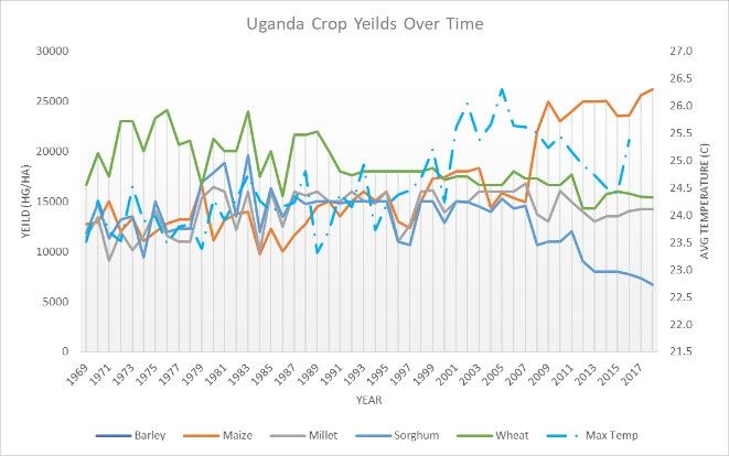
Prior work has shown that global climate models project increases in both the mean and variability of annual
mean due to stronger and more frequent El Niño and La Niña events (Cai, et al., 2014; Cai, et al., 2015;
Siam & Eltahir, 2017). Given the dependence on rainfall in the region, the resulting variability of Nile River
streamflow could increase and require additional water storage capacity on the Nile and its tributaries to
utilize and control the flow and prevent the risk of flooding (Taye, Ntegeka, Ogiramoi, & Willems, 2011;
Siam & Eltahir, 2017) (Siam & Eltahir, 2017). In addition to the effects on precipitation and water supply in
the region, these drastic fluctuations in climate will bring large increases in temperature across the region,
raising the frequency, intensity, and duration of heat waves, as well as increasing evaporative demand on
the soil and on the Nile River, its tributaries, and reservoirs.

1.2. Paper Organization
      This paper is organized into four additional sections, a literature review, description of the system
structure, model output and analysis and then a conclusion section. The literature review presents a brief
introduction to system dynamics as a methodology and discusses some examples of its application to
climate change. Additionally, this section discusses the agriculture in the Blue and White Nile Basin and
the effect of hot and dry periods on crop yields. The third section focuses on the system structure and
presents the reference modes for temperature and crop yield in the region. This section also describes the
system structure through the use of causal loop diagrams that depict the reinforcing and balancing feedback
that drives the dynamic behavior. The fourth section presents the model results and the analysis of the
output. Historic data for wheat crop yields provides a reference mode to calibrate the data and this section
discusses some of the strengths and weakness of the model in this regard. Finally, the conclusion section
presents a summary of the work conducted this far and a path forward for future work in this area.

2. Literature Review
      The literature review focuses on system dynamics, agriculture in the Blue and White Nile Basins, and
the effect of hot and dry periods on crop yields in general. System dynamics provides the underlying
methodology for the paper and is used to understand how the structure of a system drives the dynamic
behavior through accumulations and causal relationships. Overall, the agriculture in the Blue and White
Nile focuses on food stocks for the region and relies on several basic crops to include barley, maize, millet,
sorghum, and wheat. This region is heavily dependent on these cereal crops for substance and any impact
to the yield of these crops can have profound impacts on the population. Finally, the literature review
discusses the effect of hot and dry days on crop yields which is the fundamental behavior that the model in
this paper captures.

2.1. System Dynamics
      System dynamics is a methodology to understand the dynamic behavior of systems using
accumulations, flows, and causal relationships within a system. It exposes the underlying structure of a
system and models the behavior over time to adjust individuals’ mental models of the system and test
potential policy alternatives. Forrester’s (1968) work describes a system as “a grouping of parts that
operate together for a common purpose”. He further classifies two types of systems: open systems, in
which external variables affect the system, or closed systems where all variables are internal to the system
(Forrester, 1961). In his book, World Dynamics, he presents an example system model of the world that
described the interrelations between population, capital investment, geographical space, natural resources,
pollution, and food production (Forrester, 1971). The behavior of a system over time is the dynamics of a
system, which are often complex and non-linear in nature because of the system’s underlying structure
(Forrester, 1961). This complexity stems from feedback within the system, time delays between decisions
and effects, and the learning process of the system (Sterman J. , Business Dynamics: Systems Thinking
and Modeling for a Complex World, 2000). These attributes of systems make them difficult to understand
and identify the cause and effect relationships without an effective model of the system.
      Within the management domain, Forrester (1961) described the potential for system dynamics to
assist decision makers understand the implications of their policies and potentially identify and mitigate
unintended consequences of their decisions. Applications of System Dynamics have provided insights
across several domains; including corporate policy, infectious disease, commodity markets, and drug
addiction, and commodity markets (Forrester, 1971). Companies and consultants have extensively used
System Dynamics for managing large, complex projects with a great deal of success. One area where
businesses utilize System Dynamics is in the development of corporate strategy and analysis of business
decisions after a crisis or complex problem triggers these shifts in business strategy. System Dynamics
assists in determining the root cause of the crisis and identifying potential consequences of alternative
courses of action (Sterman J. , Business Dynamics: Systems Thinking and Modeling for a Complex World,
2000). One of the main benefits of the system dynamics methodology is that it makes explicit causal
relationships between variables to understand how the underlying structure and accumulations affect the
behavior of the system over time.
System dynamics has been used extensively to model climate change behavior over time and
influence potential policies through a better understanding of the dynamic behavior over time. Models have
examine the impact of the accumulation of greenhouse gases on the environment and the resulting increase
in global temperature (Sterman, et al., 2012). Likewise, system dynamics provides a means to challenge
mental models of climate change and describe the magnitude of the risks associated with potential impacts
of climate change to inform policies (Sterman J. D., 2011). In addition to the general application of system
dynamics to climate change; specific work has focused on the impact of climate on crop yields and
agricultural production in various regions, to include Africa (Stephens, et al., 2012).
2.2. Agriculture in the Blue and White Nile Basins
Rain-fed agriculture dominates water use in the Nile Basin outside Egypt, which relies almost
exclusively on irrigation. The major crops are cotton, rice, wheat, maize, sugar (cane and beet), berseem
(alfalfa), beans, fruits and vegetables. Seventy percent of the population throughout the Nile Basin can be
classified as subsistence farmers. This makes the region exceptionally vulnerable to climate extremes that
can decrease precipitation in the region as this change drastically increases the probability of wide spread
famine and unrest in the Nile Basin.
In Ethiopia, the agricultural sector dominates economic production, representing 50% of GDP, 90% of
exports (coffee, hides, live animals,vegetables), and 80% of manufacturing. Small-scale farmers produce 90%
of agricultural output, such as cereals (teff, maize, barley, wheat), pulses and oilseeds. Drought and food
insecurity regularly affects over 50% of the population, with over 90% of these people concentrated in rural
areas.
Agriculture dominates the Ugandan economy and society, contributing 44% of total output and
employing 80% of the labor force. Production is concentrated in the south, with two growing seasons.
Domestic food crops are roots and tubers, maize, beans, sesame and sorghum.Uganda is the leading coffee
producer in Africa. However, coffee and other cash crops (cotton, tea and maize) are vulnerable to climate
and international markets.
2.3. Effect of Hot and Dry Days on Crop Yields
Climate extremes—particularly hot and dry years—can reduce crop yields and result in acute water
scarcity. These risks are particularly pronounced in the Upper Nile Basin, a chronically water stressed
agricultural region that includes western Ethiopia, South Sudan, and Uganda. While the causes of
humanitarian crises in the Nile Basin are complex and involve governance, conflict, and climate, nearly all
recent regional crop failures have occurred amid hot and dry conditions (Coffel, et al., 2019).
Hot and dry years can be defined as those conditions consistent with years of poor agricultural yield:
temperatures above the 83rd percentile and precipitation below the 20th percentile (Coffel, et al., 2019).
Regional water scarcity will continue to be a chronic issue for the Upper Nile from population growth alone,
but runoff deficits during future hot and dry years will amplify this effect, leaving an additional 5–15% of the
future population facing water scarcity. Climate change, along with the region's complex water politics,
dependence on subsistence agriculture, and history of geopolitical instability, places the region at risk of
severe food and water shortages as hot and dry years become more frequent. Adaptation and climate‐
resilient water management policies informed by an understanding of compound extremes will be essential
to manage these risks.3. System Structure
This section presents the behavior and structure of the agricultural system in the Blue and White Nile
River Basins. For the Blue Nile, the data focuses on the crop yields, maximum temperature, and
precipitation in Ethiopia. For the White Nile, the section uses data from Uganda on the same crops and
weather variables. The next portion of the section discusses the causal relationships in the system that
generate the dynamic behavior for crop yields in the region. Finally, this section discusses the stock and
flow structure of the system that provides the basis for modeling efforts of the dynamic behavior of the
system.
3.1. Reference Modes
System Dynamics focuses on the behavior of a system over time and a critical component of
identifying and understanding this behavior is through the use of reference modes. Reference modes are
representations of data over time that depict how the system behaves and can generally be classified into
one of several standard reference modes (Sterman J. , Business Dynamics: Systems Thinking and
Modeling for a Complex World, 2000). Often these reference modes include oscillation which indicates that
there may be delays in the system which result in the observed behavior as the system takes time to self-
correct.
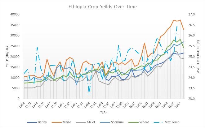
Figure 1 presents the reference modes for Ethiopia from 1969 until 2018 and includes both data on
crop yields and temperature. The data for crop yields captures the primary food crops for the region which
includes barley, maize, millet, sorghum, and wheat. The Food and Agriculture Organization (FAO) of the
United Nations maintains a robust database of crop yields across the globe, which provided the data for
the reference modes in this paper (United Nations, 2021). For Ethiopia, crop yields appear to be growing
over time, especially since 2004; however, they do demonstrate some oscillation over time. The maximum
average monthly temperature is captured on the secondary access of the chart and provides a potential
cause to the fluctuations in crop yield (World Bank Group, 2021).
Figure 2 presents similar data for Uganda for both the yield data from the FAO and climate data from
the World Bank Group. It includes the same crops that were presented for Ethiopia over the same
timeframe; however, for Uganda the crop yields do not appear to grow in a similar fashion. Additionally,
there is a sharp increase in Maize in 2007 as Sorghum drops off after a relatively steady yield rate from
1969 to 2006. This behavior indicates that there might be reinforcing behavior for crops that tend to do
well, or poorly, that eventually effects their yield rates. In both instances, Ethiopia and Uganda it is
extremely difficult to identify any trends and further analysis is needed to represent a reference mode for
modeling.
Figure 1: Crop Yield and Temp in Ethiopia (1969-2018) Figure 2: Crop Yield and Temp in Uganda (1969-2018)
Coffel et al. (2019) introduced the concept of analyzing the impact of dry-hot years on the crop yield
and used a normalized crop yield for the region. For this analysis, the paper continues to focus on Ethiopia
and Uganda; however, it limits the crops to only wheat through the modeling process. For Ethiopia, thewheat yield is growing exponentially, indicating reinforcing feedback in the system that masks the impact
of dry and hot periods on the yield. Figure 3 presents the normalized crop yield deviations for wheat in
Ethiopia and the number of dry and hot months in the year. The analysis identifies a hot or dry month as
any month where the temperature is greater than one standard deviation from the mean or precipitation is
one standard deviation less than the mean for the month. It also depicts the Ethiopian Civil War from 1974
to 1991 with the eventual independence of Eritrea in 1993, which coincides with a large decrease in the
normalized crop yields. Also, between 1995 and 2012, a series of years with both hot and dry periods
coincides with crop yields well below the normalized yield.
Figure 3: Normalized Crop Yields and Hot/Dry Months for Ethiopia
For Uganda, there are similar trends for both the number of dry and hot months as well as its impact
on the normalized yield. In the case of Uganda, the actual crop yield for wheat is trending downwards,
especially from 2000 to 2016, which coincides with a significant number of months that are dry and hot.
Figure 4 presents the normalized yield deviation and the number of days that are hotter or dryer than normal
for Uganda. It also depicts two major conflicts in Uganda, the Uganda Bush War (1980-1986) and the
Second Sudanese Civil War (1995-2005). As shown, most of the periods of low crop yields are related to
periods of dry and hot months and provide a reference mode for the yield of wheat in Uganda.
Figure 4: Normalized Crop Yields and Hot/Dry Months for Uganda3.2. Causal Relationships
Causal Loop Diagrams are a key component of system dynamics which represent the feedback
structure within a system using signed diagrams. In closed systems, casual loops differ from discrete,
event-oriented perspectives of individual causes and effects in that any cause is an effect on another
variable (Richardson, 1991). These diagrams describe the behavior of the system by talking through the
loop to tell the story of the interactions within the system (Meadows, Randers, & Meadows, 2004). Causal
loop diagrams identify the feedback structure of a system with the two types of individual feedback loops:
reinforcing and balancing loops. Richardson (1991) describes a reinforcing feedback loop as a chain of
cause and effect relationships that amplify a change in any one of the variables. A change to any variable
in the loop in one direction propagates through the loop to change the original variable in the same direction,
so these loops have the potential to grow exponentially (Meadows, Randers, & Meadows, 2004). Balancing
feedback loops work to diminish the effect of a change in a system and restore balance to a system
(Richardson, 1991). In System Dynamics, balancing feedback loops bring a system back to a desired level
or a level constrained by the system.
In natural and engineered systems delays, either information or material, often exist which increase
the dynamic complexity of these systems. These delays are generally a key contributor to the dynamic
behavior of systems and create problems, as they are difficult to capture in a mental model of the system.
In material delays conservation of matter applies, so no units will be lost during the delay, but the delay will
cause the inflow to differ from the outflow, thus resulting in an accumulation (Forrester, 1961). Whereas in
information delays, the information may lose value over time, so the accumulation of information may
diminish over time as people make decisions based on old information (Sterman J. , Business Dynamics:
Systems Thinking and Modeling for a Complex World, 2000). These delays can have dramatic effects on
a system’s behavior over time and may cause a system to overshoot is goal; potentially resulting in the
eventual collapse of the system as the growth causes irreversible damage (Meadows, Randers, &
Meadows, 2004).
Figure 3 presents the first in a series of causal loop diagrams that aid in the understanding of the
structure of the system that produces the observed dynamic behavior for crop yields in both Ethiopia and
Uganda. The “More Demand” feedback loop is a very simple reinforcing feedback loop that captures the
fact that farmers will expand the planting of successful crops. As Crop Demand increases, farmers will
increase the Area Harvested for a specific crop for both financial reasons as well as their ability to meet the
demand for food. As the Area Harvested increases, all else equal in the system, the Crop Production,
amount of crops reaped, will also increase. As Crop Production increases it will also increase the Crop
Demand for a specific crop as it become a steady part of the food system. It is likely that there is a delay,
at least a planting season long, between the Crop Demand and the Area Harvested as farmers will need
additional resources to plant a larger share of a certain crop. Not noted on this diagram is the limitation to
growth given the amount of arable land.
+
Crop Area
Demand R
Harvested
+ More Demand
Crop +
Production
Figure 5: CLD for More DemandThis is evident in the data which shows a relationship between the production of wheat in both Ethiopia
and Uganda between 1969 and 2018 (United Nations, 2021). Figure 4 presents the data for Ethiopia’s
wheat production and area harvested. The comparison of the previous year’s production to the current
year’s area harvested generates a correlation of 0.893, indicating a potential relationship between the
success of the prior year’s harvest on the area cultivated in the next year. Figure 5 presents a similar
relationship for wheat production in Uganda, where the correlation is 0.867 between the prior year’s
production amount and the next year’s area harvested. This relationship is an important aspect for
modeling the production as it demonstrates the reinforcing behavior between the production and the area
harvested.
Figure 6: Ethiopia’s wheat production and area harvested Figure 7: Uganda’s wheat production and area harvested
The next causal loop diagram captures the need for water, which could potentially balance out the
desire to plant more of a certain crop. Figure 4 presents the “Need for Water” causal diagram that is a
balancing feedback loop in the system. Previous work has documented the linkages between cultivated
land and the need for various resources to include water as a major requirement for agriculture (Turner,
Menendez, Gates, Tedeschi, & Atzori, 2016). As the Area Harvested increases, it also increases the Water
Required which in-turn decreases the Water Ratio. The Water Ratio has a positive interaction with the
Crop Yield, so when it decreases so does the Crop Yield. When the Crop Yield, the amount of a crop that
is actually harvested compared to how much is planted, decreases the Crop Production also decreases.
To complete the feedback loop, the decrease in Crop Production decreases the Crop Demand and the
Area Harvested; thus closing the loop as balancing feedback.
+
Crop Area +
Demand R Crop Area
Harvested + Demand R
Water Harvested +
+ More Demand Water
Required + More Demand
Required
B
Crop + B
Crop +
Production Need for Water
+ Production Need for Water
- +
-
Water Ratio
Water Ratio
+
Crop Yield + Profits R Crop Yield +
Technology +
Upgrade
Figure 8: CLD Need for Water +
Investment
Figure 9: CLD Technology Upgrade
Figure 5 presents the “Technology Upgrade” causal loop diagram that captures the feedback
associated with increases in technology to improve crop yield. As Crop Yield increases, so does the Crop
Production even as the Area Harvested remains constant as farmers yield more crops per acre. With anincrease in Crop Production, the Profits also begin to increase which enables farmers to increase their
Investment in technology that can improve yield. Other system dynamics modeling efforts documented a
similar structure to capture the allocation of the land to crop production and resource requirements
(Stephens, et al., 2012). After a delay for the technology to develop or be implemented, the Crop Yield
begins to increase and reinforces the initial behavior of the system.
In addition to investments in technology that may increase yield, farmers can also invest in Irrigation
to mitigate the effects of long periods without precipitation. Figure 6 presents the “Irrigation Investment”
reinforcing feedback loop that captures the feedback associated with improvements to irrigation
capabilities. As Investment increases, so does Irrigation which also increases the Water Available. The
Water Available increases the Water Ratio and improves Crop Yield. This then goes into the “Technology
Upgrade” loop as both Crop Production and Profits increase which allows for farmers to increase their
Investments. A portion of the Investment goes towards Irrigation and closes out this reinforcing feedback.
+ Water
R
Available
Irrigation
Irrigation Investment
+ +
Crop Area
Demand R
Harvested + Water
+ More Demand
Required
B
Crop +
Production Need for Water
+
- +
Water Ratio
+
Profits R Crop Yield +
Technology +
Upgrade
+
Investment
Figure 10: CLD Irrigation Investment
The final causal loop diagram describes the exogenous variable’s impact on the system structure. At
this point in the modeling effort, the El Nino Effect, which affects both the Annual Precipitation and
Temperature, is exogenous to the system. However, it is well documented that the El Nino-Southern
Oscillation directly impacts the weather patterns in the Blue and White Nile region (Giannini, Saravanan, &
Chang, 2003) (Giannini, Biasutti, Held, & Sobel, 2008). Figure 7 depicts where these variables interact
with the system and impact the overall feedback in the system. The Annual Precipitation directly relates to
Water Available in a positive manner, so as it increases so does the Water Available. However, this is not
the only affect in the model as a portion of the precipitation can be lost to run off or not captured by the
current irrigation system. The Annual Precipitation, when compared to the Normal Precipitation, also
decreases the Dry-Hot Periods as the region gets more precipitation that normal. The Temperature is
compared to the Normal Temperature to generate a Temperature Ratio, so when it is warmer than normal
this ratio increases and affects the Dry-Hot Periods. This Dry-Hot Period variable influence the Crop Yield
as found in previous work where extended periods of high temperatures and low precipitation decrease
yield (Coffel, et al., 2019).+ Water
R +
Available
Irrigation El Nino
Irrigation Investment
Effect
+ +
Crop Area
Demand R
Harvested +
Water
+ More Demand -
Required
Annual
B Precipitation
Crop +
Production Need for Water
+
- + Normal
Precipitation
Water Ratio
+ +
Profits R Crop Yield + Precipitation -
-
Technology + Ratio
Upgrade
+
+ Dry-Hot -
Temperature
Investment Periods
+
Temperature +
Ratio - Normal
Temperature
Figure 11: CLD Overall System Structure
3.3. Stock and Flow Structure
This section presents and discusses the stock and flow structure of the model that drives the dynamic
behavior of the system and helps to better understand the includes two sub-models that focus on the impact
of El Nino and La Nina on dry-hot periods in the region and the other focuses on the crop yield and
production in the region. For this model, the stock and flow structure only models the behavior of Wheat,
one of the primary food crops in the region. Additionally, the model represents one country in the region
based on the initial conditions which can be altered and calibrated to capture the behavior of other countries.
One of the important aspects of the model is the impact of El Nino and La Nina have on the region’s
temperature and precipitation. In times of La Nina, a cooling of the Pacific Ocean, the Nile River Basin
experiences increased temperatures and decreased amounts of precipitation (Siam, Wang, Demory, &
Eltahir, 2014). Additionally, these events are becoming more frequent and increasing in intensity, leading
to longer periods of drought in the region (Cai, et al., 2015). NOAA tracks the average temperatures of the
Pacific Ocean to measure the El Nino-Southern Oscillation with a three-month moving average temperature
and any period that is +/- 0.5° C is considered a Nino event (National Weather Service, 2021).
Figure 12 presents a summary of this data and indicates the El Nino periods, greater than + 0.5° C,
and La Nina periods, less than -0.5° C. For the purposes of modeling the dynamic behavior of the system,
the Nino effect is considered exogenous to the model and the El Nino Southern Oscillation Effect variable
captures this behavior.Figure 12: Oceanic Nino Index from 1969 to 2018 (National Weather Service, 2021)
Figure 13 presents the stock and flow structure for the Dry-Hot Periods which captures the impact of
the El Nino Southern Oscillation Effect on the Temperature and Precipitation in the region which results in
the Dry-Hot Periods. In general, the ocean temperatures fluctuate by about +/- 1.5° C during periods of El
Nino or La Nino and the model captures this level of fluctuation (National Weather Service, 2021). The
current model does not capture the observed increase in frequency or intensity of the effect; however, this
could be added as the model matures (Cai, et al., 2015). The model then determines if a given period is
hot, Temperature greater than one standard deviation from the Average Temperature, or dry, Precipitation
less than one standard deviation from the Average Precipitation. When both conditions are met, the period
is designated as Dry and Hot and begins to accumulate in the Dry-Hot Periods.
Time for
Temperature
Change Impact
-
Temperature El Nino Temperature
Change in
Change
Temperature
+ +
Temperature -
- - +
Ratio Temperature
Gap La Nina Effect on +
+ + Temperature
Time to Reset Average El Nino Southern
Dry-Hot Temperature Oscillation Effect
- +
+
Dry-Hot Periods El Nino Ocean
Average
Decrease in Increase in Temperature Change
Precipitation
Dry-Hot Periods Dry-Hot Periods
+ +
+ + La Nina Effect on +
- Precipitation Precipitation
Precipitation
Dry-Hot Period Gap +
Ratio +
Time -
+ El Nino Precipitation
+ Change
Precipitation
Change in
Precipitation
-
Time for
Precipitation
Change Impact
Figure 13: Stock and Flow Diagram for Dry-Hot Periods
The second portion of the stock and flow model focuses on the crop yield for wheat in a given country
and the resulting crop production. Figure 14 presents the stock and flow model for this portion of the system
and include three stocks for the Crop Yield – Wheat, Area Harvested – Wheat, and the Desired Area
Harvested – Wheat. The desired area harvested is based on the amount of production, so as the region
produces more wheat, farmers in the region will want to plan more of the crop to take advantage of thesuccess. However, this takes some time to both adjust the desired area harvested as well as the actual
area harvested, so the model uses two delays to capture this behavior. The Crop Production – Wheat
variable is the product of both the yield and the amount harvested and can be calibrated to historic
production in the country.
Decrease in Wheat
Crop Yield - Dry-Hot
Period
Fractional Increase
in Wheat Yield
+
Fractional
Time to adjust Area Decrease in Wheat
Yield Normal Fractional
Harvested - Wheat + + +
Crop Yield - Increase in Wheat
Net Decrease Wheat Net Increase Yield
- Wheat Yield Wheat Yield
Area Harvested
+
- Wheat +
Change in Area
+
Harvested - Wheat
+ Crop Production
- Wheat
+
Initial Crop Yield - Wheat
Area Harvested +
Gap - Wheat - -
+ R Crop Production
Increase - Wheat
+
Initial Crop
Production - Wheat
+ + +
Area Harvested
Relative to Production
Desired Area - + - Wheat
Harvested - Wheat
Change in Desired
Area - Wheat Initial Area Harvested - Wheat
-
Time to adjust
Desired Area - Wheat
Figure 14: Stock and Flow Diagram for Crop Yield
The structure in Figure 13 and Figure 14 is linked through the Dry-Hot Period stock in Figure 13’s
model and the Decrease in Wheat Crop Yield – Dry-Hot Period variable in Figure 14’s portion of the model.
As the number of dry-hot periods increase it also decreases the rate at which the crop yield decreases by
affecting the fractional decrease in wheat yield. So, as more dry-hot periods occur and become more
severe, the crop yield for wheat decreases. During dry-hot periods, the crop yield of sustenance crops, like
wheat, decreases due to the drought conditions in the area (Coffel, et al., 2019).
There are some shortcomings in the model that need to be refined to improve the accuracy of the
model in representing the crop yield in the Nile River Basin. The focus of this model was on the impact of
rainfall and temperature, which appear to be major contributing factors to crop yield in the area; however,
it does not examine infestations, improvements in technology, fertilizers, or insecticides. This leaves room
for improvement in the model and the subsequent analysis. First, the growth of the crop yield is currently
an exogenous variable based on historic growth rates of the wheat yield in Ethiopia and Uganda. The
model could be improved to account for improvements in technology or irrigation in the region, fueled by
increased production and thus profits. Likewise, further research could identify other causes of decreases
to crop yield, something like conflict in the region, which may affect production. As noted earlier, the final
model improvement could incorporate the increase in the frequency and severity of the El Nino periods
which result in increased periods of drought in the region, like observed in the 1990s.
4. Model Results and Analysis
Overall, the model generates consistent behavior with historic data for the crop yield of both Ethiopia
and Uganda. Although it is a relatively basic model for understanding the impact of dry-hot periods on the
crop yield for these countries, by calibrating the model with the fractional increase in decrease in wheat
yield the model output is similar to historic data. The FAO data from the United Nations provides anexcellent reference mode for the model and depicts the impact that dry-hot periods can have on the region’s
production of Wheat.
4.1. Ethiopia – Wheat
Ethiopia’s crop yield for wheat has been growing exponentially over the last several decades and the
area harvested has also been increasing as depicted in the previous section. Figure 15 presents the model
output for the crop yield for wheat in Ethiopia, which increases over time with some oscillation that aligns
with dry-hot periods in Ethiopia driven by the El Nino Southern Oscillation. Overall, the model’s output of
the crop yield follows the historic data very closely. Figure 16 presents the area harvested for wheat in
Ethiopia from 1969 to 2018 for both the historic data and the model. The output for the area harvested,
specifically for wheat, does not follow the historic data quite as well as it does not capture a large decrease
from 1977 to 1994; however, the general trend is similar.
Crop Yield Area Harvested - Wheat
30,000 2M
22,500 1.5 M
Hectagram/Hectacre
Hectacre
15,000 1M
7500 500,000
0 0
1969 1977 1985 1994 2002 2010 2019 1969 1977 1985 1994 2002 2010 2019
Date Date
Baseline Historic Baseline Historic
Figure 15: Model Output - Ethiopia Wheat Yield Figure 16: Model Output - Ethiopia Wheat Area Harvested
4.2. Uganda - Wheat
Uganda’s wheat yield remains relatively consistent over time with a slight decrease from 1969 to 2018;
however, it is much higher than the yield in Ethiopia. Figure 17 presents the wheat yield for Uganda and
compares the model baseline output with the historic data. Similar to Ethiopia, the oscillation of the yield is
not quite as severe in the model but follows the general trend of the historic data. Figure 18 presents the
area harvested for wheat, which for Uganda is somewhat consistent from 1969 to 2000, but then grows
rapidly after 2000. This indicates that there may be additional structure in the system that the model does
not capture that may be driving the behavior for the area harvested.
Crop Yield Area Harvested - Wheat
30,000 20,000
22,500 15,000
Hectagram/Hectacre
Hectacre
15,000 10,000
7500 5000
0 0
1969 1977 1985 1994 2002 2010 2019 1969 1977 1985 1994 2002 2010 2019
Date Date
Baseline Historic Baseline Historic
Figure 17: Model Output - Uganda Wheat Yield Figure 18: Model Output - Uganda Wheat Area Harvested
One area where the model could be improved is in capturing the magnitude of fluctuations of the crop
yield in both Ethiopia and Uganda based on the El Nino Southern Oscillation. It is well documented that
the crop yields in the region are highly related to dry-hot periods which can greatly affect the crop yield forthese food crops (Coffel, et al., 2019). The model does capture some of the oscillation, but not quite to the
extent that is evident in the historic data which may be important for future analysis of the impact of the
decrease in crop yield on the population.
5. Conclusions
This paper presents an adaptable system dynamics model of the crop yield, specifically for wheat, in
the Upper Nile Basin countries of Ethiopia and Uganda. It models the documented relationships between
dry-hot periods and decreased crop yields in the area and provides calibrated output for both countries.
Additionally, it shows some relationships between the success of a crop yield and the area harvested as
seen in the reference modes from historic data. Overall, it provides a basis for further analysis to identify
potential impacts to population and risk for conflict in the region.
5.1. Key Takeaways
The causal relationship between hot and dry periods on crop production is well documented and
historic data provides a means to validate the model of crop production for a given country. Although the
model presented is relatively simplistic in its structure, it is able to model the historic behavior of wheat
production and yield in both Ethiopia and Uganda. The model does take into account the fluctuations in
temperature and precipitation brought on by the El Nino Southern Oscillation in the region; however, it does
not accurately reflect the magnitude of this effect and could be improved in future iterations of the model.
Additionally, the model does not account for the observed increase in both frequency of El Nino events or
the intensity of these events that has been observed in recent years.
5.2. Future Work
Future work in this area will focus on three major areas: first to expand the current model to incorporate
other cereal crops in the region to include barley, maize, sorghum, and millet; and second to improve the
accuracy of the area harvested model by identifying additional causal relationships; and finally, to determine
and model the impact of poor crop yields on the population. The model in this paper solely focuses on
wheat in the two countries and provides a basis for modeling other cereal crops that are essential to the
region. Additionally, there will be feedback loops between the various crops that may impact the area
harvested as there is a limited amount of arable land in the region. Currently, the model does not closely
model the historic behavior for the area harvested for wheat in Uganda, potentially because of missing
relationships for the demand for crops that should be addressed by future work. The final piece of future
work will be the most important aspect of the model which will identify when the climate induced affects on
crop yield begin to impact the population in the region and potentially lead to conflict. The aim of the final
model will be to inform decision makes on the importance of countering the effects of climate change in the
region or at least mitigating the effect on future crop yields as the population doubles in the next thirty years.
References
African Union. (n.d.). African Union Food Security. Addis Ababa.
Asseng, S., Kheir, A. M., Kassie, B. T., Hoogenboom, G., Abdelaal, A. I., Haman, D. Z., & Ruane, A. C.
(2018). Can Egypt become self-sufficient in wheat? Environmental Research Letters, 13(9).
doi:10.1088/1748-9326/aada50
Broad, K., & Agrawala, S. (2000). The Ethiopia food crisis--uses and limits of climate forecasts. Science,
289(5485), 1693-1694. doi:10.1126/science.289.5485.1693
Burrows, K., & Kinney, P. L. (2016). Exploring the Climate Change, Migration and Conflict Nexus.
International Journal of Environmental Research and Public Health, 13(4).
doi:10.3390/ijerph13040443Cai, W., Borlace, S., Lengaigne, M., van Rensch, P., Collins, M., Vecchi, G., . . . Jin, F.-F. (2014).
Increasing frequency of extreme El Niño events due to greenhouse warming. Nature Climate
Change, 4(2), 111-116. doi:10.1038/nclimate2100
Cai, W., Wang, G., Santoso, A., McPhaden, M. J., Wu, L., Jin, F.-F., . . . Guilyardi, E. (2015). Increased
frequency of extreme La Niña events under greenhouse warming. Nature Climate Change, 5(2),
132-137. doi:10.1038/nclimate2492
Coffel, E., Keith, B., Lesk, C., Horton, R., Bower, E., Lee, J., & Mankin, J. (2019). Future Hot and Dry
Years Worsen Nile Basin Water Scarcity Despite Projected Precipitation Increases. Earth's
Future(7). doi:10.1029/2019EF0012
Department of Economic and Social Affairs. (2013). World Population Prospects: The 2012 Revision -
Volume I: Comprehensive Tables. New York: United Nations.
Forrester, J. W. (1961). Industrial Dynamics. Waltham, MA: Pegasus Communications Inc.
Forrester, J. W. (1968). Principles of Systems. Cambridge, MA: Wright-Allen Press, Inc.
Forrester, J. W. (1971). World Dynamics. Cambridge, MA: Wright-Allen Press, Inc.
Giannini, A., Biasutti, M., Held, I. M., & Sobel, A. H. (2008). A global perspective on African climate.
Climatic Change, 90(4), 359-383. doi:10.1007/s10584-008-9396-y
Giannini, A., Saravanan, R., & Chang, P. (2003). Oceanic Forcing of Sahel Rainfall on Interannual to
Interdecadal Time Scales. Science, 302(5647), 1027-1030. doi:DOI: 10.1126/science.1089357
Keith, B., Ford, D. N., & Horton, R. (2017). Considerations in managing the fill rate of the Grand Ethiopian
Renaissance Dam Reservoir using a system dynamics approach. The Journal of Defense
Modeling and Simulation, 14(1), 33-43. doi:10.1177/1548512916680780
Kent, C., Pope, E., Thompson, V., Lewis, K., Scaife, A. A., & Dunstone, N. (2017). Using climate model
simulations to assess the current climate risk to maize production. Environmental Research
Letters, 12(5). doi:10.1088/1748-9326/aa6cb9
Kim, U., & Kaluarachchi, J. J. (2009). Climate Change Impacts on Water Resources in the Upper Blue
Nile River Basin, Ethiopia. Journal of the American Water Resources Association, 45(6), 1361-
1378. doi:10.1111/j.1752-1688.2009.00369.x
Lesk, C., Rowhani, P., & Ramankutty, N. (2016). Influence of extreme weather disasters on global crop
production. Nature, 529, 84-87. doi:10.1038/nature16467
Lobell, D. B., Bänziger, M., Magorokosho, C., & Vivek, B. (2011). Nonlinear heat effects on African maize
as evidenced by historical yield trials. Nature Climate Change, 1(1), 42-45.
doi:10.1038/nclimate1043
Matiu, M., Ankerst, D. P., & Menzel, A. (2017). Interactions between temperature and drought in global
and regional crop yield variability during 1961-2014. PLoS One.
doi:10.1371/journal.pone.0178339
Meadows, D., Randers, J., & Meadows, D. (2004). Limits to Growth: The 30-year Update. White River
Junction, VT: Chelsea Green Publishing Company.
National Weather Service. (2021, March 4). Cold & Warm Episodes by Season. Retrieved March 10,
2021, from Climate Prediciton Center:
https://origin.cpc.ncep.noaa.gov/products/analysis_monitoring/ensostuff/ONI_v5.php
Richardson, G. P. (1991). Feedback Thought in Social Sciences and Systems Theory. Philadelphia, PA:
University of Pennsylvania Press.
Siam, M. S., & Eltahir, E. A. (2017). Climate change enhances interannual variability of the Nile river flow.
Nature Climate Change, 7(5), 350-354. doi:10.1038/nclimate3273
Siam, M. S., Wang, G., Demory, M.-E., & Eltahir, E. A. (2014). Role of the Indian Ocean sea surface
temperature in shaping the natural variability in the flow of Nile River. Climate Dynamics, 43(3),
1011-1023. doi:10.1007/s00382-014-2132-6
Stephens, E., Nicholson, C., Brown, D., Parsons, D., Barrett, C., Lehmann, J., . . . Riha, S. (2012).
Modeling the impact of natural resource-based poverty traps on food security in Kenya: The
Crops, Livestock and Soils in Smallholder Economic Systems (CLASSES) model. Food Security,
4(3), 423-439. doi:10.1007/s12571-012-0176-1Sterman, J. (2000). Business Dynamics: Systems Thinking and Modeling for a Complex World. Boston,
MA: Irwin McGraw-Hill.
Sterman, J. D. (2011). Communicating climate change risks in a skeptical world. Climatic Change, 108(4),
811-826. doi:10.1007/s10584-011-0189-3
Sterman, J., Fiddaman, T., Franck, T., Jones, A., McCauley, S., Rice, P., . . . Siegel, L. (2012). Climate
interactive: the C‐ROADS climate policy model. System Dynamics Review, 28(3), 295-305.
doi:10.1002/sdr.1474
Taye, M. T., Ntegeka, V., Ogiramoi, N. P., & Willems, P. (2011). Assessment of climate change impact on
hydrological extremes in two source regions of the Nile River Basin. Hydrol. Earth Syst. Sci.,
15(1), 209-222. doi:10.5194/hess-15-209-2011
Turner, B. L., Menendez, H. M., Gates, R., Tedeschi, L. O., & Atzori, A. S. (2016). System Dynamics
Modeling for Agricultural and Natural Resource Management Issues: Review of Some Past
Cases and Forecasting Future Roles. Resources, 40(5). doi:10.3390/resources5040040
United Nations. (2021, February 01). FAO STAT. Retrieved February 15, 2021, from Food and
Argriculture Organization of the United Nations: http://www.fao.org/faostat/en/#home
World Bank Group. (2021). Climate Change Knowledge Portal. Retrieved March 1, 2021, from
https://climateknowledgeportal.worldbank.org/country/guinea/climate-data-historical
Zscheischler, J., Westra, S., van den Hurk, B. J., Seneviratne, S. I., Ward, P. J., Pitman, A., . . . Zhang, X.
(2018). Future climate risk from compound events. Nature Climate Change, 8(6), 469-477.
doi:10.1038/s41558-018-0156-3You can also read