Modélisation hybride RANS/DVMS autour d'obstacles statique et tournants - RESEARCH REPORT N 9464
←
→
Page content transcription
If your browser does not render page correctly, please read the page content below
Modélisation hybride
RANS/DVMS autour
d’obstacles statique et
tournants
Florian Miralles, Bastien Sauvage, Stephen Wornom, Bruno Koobus,
Alain Dervieux
                                                                   ISRN INRIA/RR--9464--FR+ENG

RESEARCH
REPORT
                                                                   ISSN 0249-6399

N° 9464
2022
Project-Team Ecuador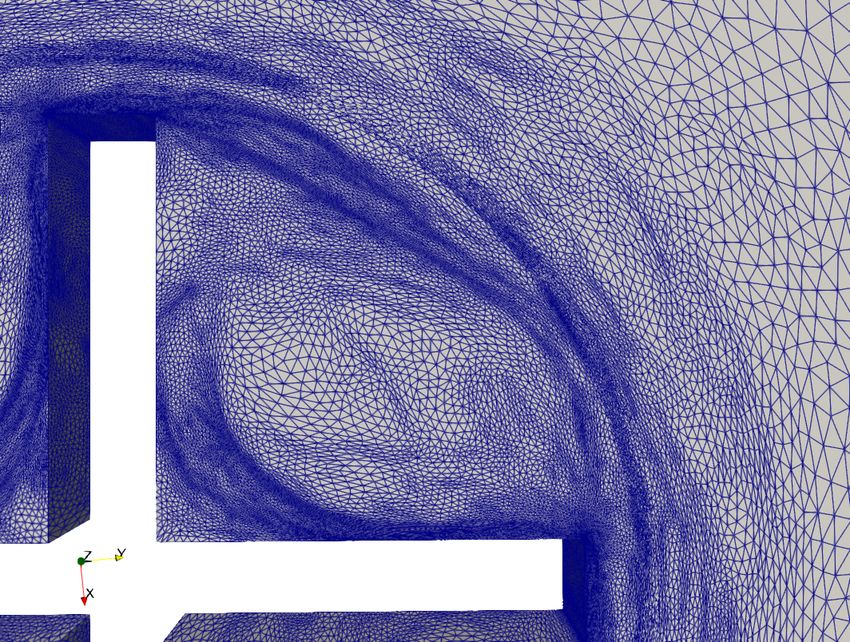
Modélisation hybride RANS/DVMS autour
                         d’obstacles statique et tournants

                  Florian Miralles ∗ , Bastien Sauvage † , Stephen Wornom ‡ , Bruno
                                            Koobus § , Alain Dervieux ¶
                                               Équipe-Projet Ecuador

                                Rapport de recherche n° 9464 — 2022 — 26 pages

       Résumé : Nous examinons la modélisation hybride RANS-LES pour l’étude des écoulements
       autour des machines tournantes comme les hélicoptères et les drones. En utilisant un maillage fin,
       les simulations devraient fournir des estimations précises concernant l’émission de bruit. Chacun de
       ces écoulements peut impliquer des régions turbulentes moyennes et hautes de Reynolds avec des
       tourbillons détachés et avec de fines couches limites laminaires et turbulentes. Un modèle hybride,
       comme le DDES, est alors obligatoire, avec éventuellement une résolution améliorée des régions
       LES, qui sont principalement des sillages turbulents. Il est alors intéressant d’appliquer dans ces
       régions un modèle LES plus sophistiqué que la partie LES de DDES. Dans notre étude, nous
       utilisons le modèle multi-échelle variationnel dynamique (DVMS). Dans les autres régions, une
       modélisation DDES ou simplement une modélisation RANS est appliquée. Dans les deux cas, une
       fermeture à deux équations est choisie. Après une discussion des ingrédients de la modélisation, nous
       présenterons une comparaison des modèles RANS, LES et hybrides pour deux séries d’écoulements.
       Bien que calculés par de nombreux chercheurs, les écoulements autour des cylindres restent difficiles
       à prévoir. La comparaison se poursuivra avec un écoulement autour d’un mélangeur en forme de
       croix tournant à l’intérieur d’un cylindre. Ce rapport est une version plus longue de [23]. Ce travail
       a été soutenu par le projet ANR NORMA dans le cadre de la subvention ANR-19-CE40-0020-01.
       Mots-clés : modèles hybrides de turbulence, modèle variationnel multi-échelle pour LES, méthode
       chimera, écoulement autour d’un cylindre, machine tournante, grilles non structurées

    ∗ IMAG, Univ. Montpellier, CNRS, Place Eugène Bataillon, 34090 Montpellier, France. E-mail:

florian.miralles@umontpellier.fr
    † Univ. Côte d’Azur/INRIA Projet Ecuador, Sophia-Antipolis, France, E-mail: Bastien.Sauvage@inria.fr
    ‡ IMAG, Univ. Montpellier, CNRS, Montpellier, France. E-mail: stephen.wornom@inria.fr
    § IMAG, Univ. Montpellier, CNRS, Montpellier, France. E-mail: bruno.koobus@umontpellier.fr
   ¶ Lemma, Biot, France, and Univ. Côte d’Azur/INRIA Projet Ecuador, Sophia-Antipolis, France, E-mail:

alain.dervieux@inria.fr

          RESEARCH CENTRE
          SOPHIA ANTIPOLIS – MÉDITERRANÉE

          2004 route des Lucioles - BP 93
          06902 Sophia Antipolis Cedex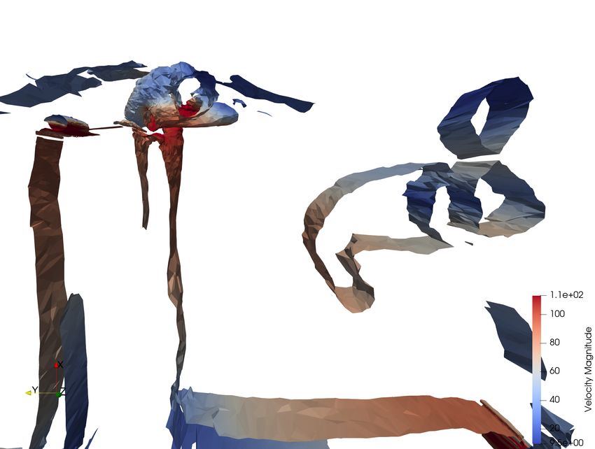
Hybrid RANS/DVMS modeling for static and rotating
                     obstacles
Abstract: We examine hybrid RANS-LES modeling for the study of flows around rotating
machines like helicopters and drones. Using a fine-mesh, the simulations should provide accurate
estimates concerning the noise emission. Each of these flows can involve mean and high Reynolds
turbulent regions with detached eddies and with thin laminar and turbulent boundary layers.
A hybrid model, like DDES, is then mandatory, with possibly an improved resolution of LES
regions, which are mainly turbulent wakes. It is then interesting to apply in these regions a
more sophisticated LES model than the LES part of DDES. In our study, we use the dynamic
variational multiscale model (DVMS). In the other regions, a DDES or simply a RANS modeling
is applied. In both cases a two-equation closure is chosen. After a discussion of the modeling
ingredients, we shall present a comparison of the RANS, LES, and hybrid models for two series
of flows. Although computed by many researchers, flows around cylinders remain difficult to
predict. The comparison will continue with a flow around a cross shaped mixing device rotating
inside a cylinder. This report is a longer version of [23]. This work was supported by the ANR
project NORMA under grant ANR-19-CE40-0020-01.
Key-words: hybrid turbulence models, variational multiscale model for LES, chimera method,
cylinder flow, rotating machine, unstructured grids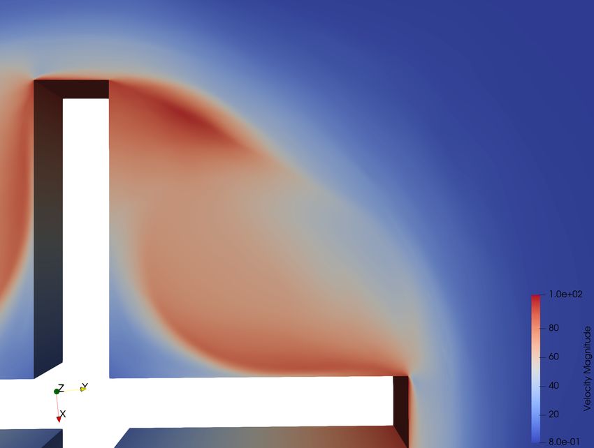
Hybrid RANS/VMS                                                                                                                                                 3

Table des matières
1 Introduction                                                                                                                                                  5

2 Turbulence modeling                                                                                                                                           5
  2.1 RANS . . . . . . . . . . . .     .   .   .   .   .   .   .   .   .   .   .   .   .   .   .   .   .   .   .   .   .   .   .   .   .   .   .   .   .   .    5
  2.2 DDES model . . . . . . . .       .   .   .   .   .   .   .   .   .   .   .   .   .   .   .   .   .   .   .   .   .   .   .   .   .   .   .   .   .   .    7
  2.3 High Reynolds computation        .   .   .   .   .   .   .   .   .   .   .   .   .   .   .   .   .   .   .   .   .   .   .   .   .   .   .   .   .   .    8
  2.4 LES-like model : DVMS . .        .   .   .   .   .   .   .   .   .   .   .   .   .   .   .   .   .   .   .   .   .   .   .   .   .   .   .   .   .   .    8
      2.4.1 SGS model . . . . .        .   .   .   .   .   .   .   .   .   .   .   .   .   .   .   .   .   .   .   .   .   .   .   .   .   .   .   .   .   .    9
      2.4.2 DVMS . . . . . . . .       .   .   .   .   .   .   .   .   .   .   .   .   .   .   .   .   .   .   .   .   .   .   .   .   .   .   .   .   .   .   10
  2.5 Hybrid RANS/DVMS . . .           .   .   .   .   .   .   .   .   .   .   .   .   .   .   .   .   .   .   .   .   .   .   .   .   .   .   .   .   .   .   12
  2.6 Hybrid DDES/DVMS . . .           .   .   .   .   .   .   .   .   .   .   .   .   .   .   .   .   .   .   .   .   .   .   .   .   .   .   .   .   .   .   13

3 Numerical discretization                                                                                                                                     13
  3.1 Numerical scheme . . . . . . . . . . . . . . . . . . . . . . . . . . . . . . . . . . .                                                                   13
  3.2 Mesh adaptation for rotating machines . . . . . . . . . . . . . . . . . . . . . . . .                                                                    15

4 Applications                                                                                                                                                 16
  4.1 Flow past a cylinder . . . . . . . . . . . . . . . . . . . . . . . . . . . . . . . . . .                                                                 16
  4.2 Flow around a rotating cross . . . . . . . . . . . . . . . . . . . . . . . . . . . . .                                                                   23

5 Conclusion                                                                                                                                                   23

RR n° 9464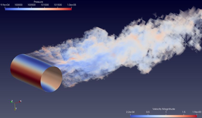
4                                                                        Miralles

NOMENCLATURE

    W         [−]         flow variables
    ρ         [kg/m3 ]    density
    u         [m/s]       velocity vector
    E         [J/m3 ]     total energy per unit volume
    k         [m2 /s2 ]   turbulence kinetic enery
    ε         [m2 /s3 ]   dissipation rate of k
    Wh        [−]         discrete flow variables
    W 0h      [−]         small resolved scales of W h
    h i       [−]         Reynolds average
    F         [−]         convective and diffusive fluxes
    τ RAN S   [−]         RANS closure term
    τ LES     [−]         LES closure term
    τ DDES    [−]         DDES closure term
    ν         [m2 /s]     kinematic viscosity of the fluid
    νt        [m2 /s]     turbulent kinematic viscosity
    Cd        [−]         mean drag coefficient
    Cl0       [−]         r.m.s. of the lift coefficient
    C pb      [−]         mean base pressure coefficient
    θ         [deg.]      mean separation angle
    ∆         [m]         LES filter width
    lRAN S    [m]         RANS turbulence length scale
    µSGS      [kg/m/s]    LES eddy viscosity
    µRAN S    [kg/m/s]    RANS eddy viscosity
    τe        [-]         Reynolds stress tensor
    Sets
    Ωf                    Fluid domain
    Ωh                    Collection of Tetrahedron
    Jk                    Index set wich are contains in macro cell Ck
    Ck                    Agglomeration cell
    V2h                   the space of large scales
     0
    Vh                    the space of small scales

                                                                            Inria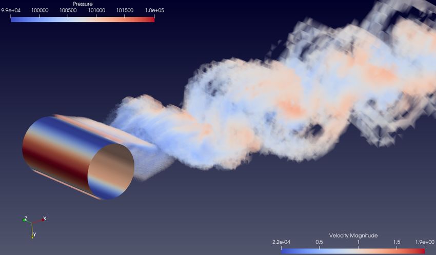
Hybrid RANS/VMS                                                                                   5

1     Introduction
     In this paper, hybrid models are evaluated for the simulation of massively separated flows
around fixed and moving geometries, with the objective of applying them to aeroacoustic problems
involving complex industrial flows at high Reynolds numbers. For this purpose, the turbulence
models need to behave preferentially like large eddy simulation models (LES) in order to introduce
little dissipation and thus better capture the small scales and the fluctuations of the unsteady
flows considered. However, these flows involve very thin boundary layers, which current computers
and softwares cannot compute in LES mode, only in RANS mode. To accommodate both needs,
LES and RANS, the hybrid turbulence approach, combining LES and RANS in a somewhat
zonal manner, is considered by many research teams.
     In this work, beside the classical Delayed Detached Eddy Simulation model (DDES, [32]),
we study an approach which combines zonally this last model and the dynamic variationnal
multiscale model (DVMS, [19]). In this hybrid DDES/DVMS approach [24], the DVMS model
is preferentially activated in the wake regions where this latter model introduces less dissipation
than the LES component of DDES. A hybrid RANS/DVMS model [16], where the RANS
component is Goldberg’s k − ε model [10], is also applied in this study. A smooth blending
function, which is based on the value of a blending parameter, is employed in these hybrid
strategies, for switching from RANS to DVMS or DDES to DVMS. In [16], these models are
applied to flows around a cylinder at moderate Reynolds number, starting from Reynolds number
20000.
In many industrial cases, and particularly cases with rotating geometries like propellers, the
Reynolds number is much higher.
     In the present paper, these hybrid models are applied to the flow around a circular cylinder
in the supercritical regime, namely at Reynolds numbers 1 million and 2 million. At Reynolds
number 1 million, the supercritical regime shows turbulent flow separation on both the upper
and lower surface of the cylinder with a laminar-turbulent transition in the boundary layers
located between the stagnation point and the separation one. At Reynolds number 2 million, the
high transition regime shows a fully turbulent boundary layer on one side of the cylinder, and a
partially laminar, partially turbulent boundary layer on the other side. This benchmark, which
contains many characteristics encountered in industrial flows, is challenging due to the complex
physics of the flow and the considered high Reynolds numbers, and remains a difficult calculation
to perform. The second application concerns the flow at Reynolds number 1.8 million around a
cross shaped mixing device rotating inside a cylinder.
     This work is part of a cooperation program with Keldysh Institute of Applied Mathematics
of Moscow focussing on the “Efficient simulation of noise of rotating machines”, see e.g. [7, 3, 6].
     The remainder of this paper is organized as follows. Section 2 presents the hybrid turbulence
models used in this work. Section 3 describes the numerical scheme. In Section 4, applications
are presented. The obtained results are analyzed and compared with those obtained in other
numerical studies and with experimental data. Finally, concluding remarks are drawn in Section
4.

2     Turbulence modeling
2.1    RANS
  First, we want to specify that RANS stands for unsteady RANS throughout this document.
When comparing with other published results, we use the notation that appear in the published

RR n° 9464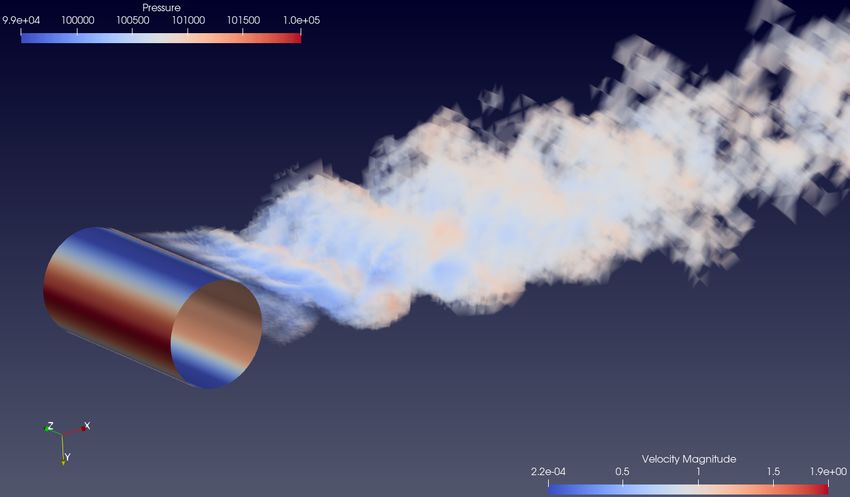
6 Miralles
articles notable URANS which is shorthand for Unsteady RANS, which the same as RANS in
this document. Steady RANS will be denoted as SRANS and Steady LES as SLES.
In this work, and as far as the closure of the RANS equations is concerned, we use the low
Reynolds k − ε model proposed in Goldberg et al.[10]. This model was designed to improve the
predictions of the standard k − ε one for adverse pressure gradient flows, including separated
flows. The equations of this model are recalled in this document, in dimensionless frame :
k2
µt = ρcµ fµ (k, ε) , (1)
ε
where the damping function is defined as follow :
!
1 − eaµ Rt (k,ε) cτ k2
fµ (k, ε) = √ max 1, p , Rt (k, ε) = Re . (2)
1 − e− Rt (k,ε) Rt (k, ε) ε
function Rµ represent the turbulent Reynolds number. Transports equation on k and ε can be
written as :
∂ρk 1 µt
+ ∇ · (ρe
uk) = τe : ∇e
u+∇· + ∇k − ρε, (3)
∂t Re σk
2
∂ρε 1 µt ε (2) ε
uε) = ∇ ·
+ ∇ · (ρe + ∇ε + c(1)ε τ
e : ∇e
u − cε ρ + C (2)
(k, ε) C (1) (k, ε).
∂t Re σε k k
(4)
Since to control production and dissipation of dissipation rate, functions C (1) and C (2) are
introduced. These functions are defined such that :
k cτ
C (k, ε) = max 1, √
(1)
,
ε Rt
1/4 ! p
√
3 1 k
(2)
C (k, ε) = ρ max k, ε εC max (∇k · ∇
(1) , 0).
10 Re ε
The total system, including the fluids variables and turbulent variables, can be written as :
∂W
∂t + ∇ · F (W ) = τ RAN S (W ),
+Boundary conditions, (5)
Q(0, x) = Q0 (x), ∀x ∈ Ωf
Where τ RAN S means the RANS closure terms, defined such that :
ρ
ρ ρu ρE ρk z }| {
2
(1) ε (2) ε
z}|{ z}|{ z}|{ z }| {
τ RAN S (W ) = (2) (1)
0 , 0 , 0 , τ
e : ∇e
u − ρ, c ε τ
e : ∇e
u − cε ρ + C (k, ε) C (k, ε)
k k
(6)
In practice, for compressible flow, we use the constants summarize in the table below :
(1) (2)
cε cε σk σε
1.44 1.92 1.0 1.3
Inria
Hybrid RANS/VMS 7
2.2 DDES model
The DDES approach used in this work is based on the Goldberg’s k − ε model [10]. In
other words, this RANS model is introduced in the DDES formulation [32] by replacing the
k3/2
DkRAN S = ρε dissipation term in the k equation by DkDDES = ρ lDDES where
k 3/2 k 3/2
lDDES = − fd × max(0, − CDDES ∆)
ε ε
with fd = 1 − tanh((8rd )3 )
νt + ν
and rd = √ .
max( ui,j ui,j , 10−10 )K 2 d2w
K denotes the von Karman constant (K = 0.41), dw the wall-normal distance, ui,j the xj -
derivative of the ith-component of the velocity u, and the model constant CDDES is set to the
standard value 0.65. We define here the DDES k − ε Goldberg source term :
ρ
ρ ρu ρE ρk z }| {
ε2
ε
z}|{ z}|{ z}|{ z }| {
τ DDES (W ) = u − DkDDES , c(1) u − c(2) + C (2) (k, ε) C (1) (k, ε)
0 , 0 , 0 , τe : ∇e ε
k
τe : ∇e ε ρ
k
(7)
Symbol ∆ holds for the filter width, in the type of LES which we use, the filter width is fixed to
the local mesh size. The definition of the local mesh size is not an easy question when (highly)
anisotropic meshes are used. Two main options are (1) the third root of the grid element volume
and (2) the largest local edge. However, our experience is that, when combined with devices like
VMS and Dynamic-LES, the choice in defining the local mesh size is not so sensitive. Our filter
width is defined as the third root of volume of the grid element T, then :
Z 1/3
∆ = ∆T = dx . (8)
T
RR n° 9464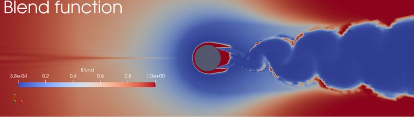
8                                                                                                             Miralles

2.3    High Reynolds computation
   In order to catch the turbulent boundary layer, we use a wall law modeling, designed by
Reichardt [27]. By this way, the no slip boundary condition on the wall become :
                                                  +
                                                        −y +
                                                                 +
                        1                         −y              −y
                   +              +
                                                                                                                   (9)

               U       = ln 1 + κy + 7.8 1 − exp      −      exp
                        κ                          11    11        3

   Also, for turbulent variables, we use the work of Jaeger [17], with the following condition on
the wall :

                                                    2
                                 u2f           y+

                              k=p                        ,
                                  Cµ           10
                                                         2         "    + 2 #!
                                     u4f            y+

                                                               0.2       y
                              ε = Re                          +p     1−           .
                                     10κ            10           Cµ      10

    The Reichardt wall law give us a smooth transition from linear to logarithmic boundary layer.

2.4    LES-like model : DVMS
    In this section, we present the DVMS model which is preferred to the classical LES approach
in our hybrid strategies because of some specific properties, as will be specified hereafter, that
allow this model to have a better behavior in some regions of the flow, such as shear layers and
wakes.
    The Variational Multiscale (VMS) model for the large eddy simulation of turbulent flows
has been introduced in [15] in combination with spectral methods. In [19], an extension to
unstructured finite volumes is defined. This method is adapted in the present work. Let us
explain this VMS approach in a simplified context. Assume the mesh is made of two embedded
meshes. On the fine mesh we have a P 1 -continuous finite-element approximation space Vh with
the usual basis functions Φi vanishing on all vertices but vertex i. Let be V2h its embedded coarse
subspace V2h . Let Vh0 be the complementary space : Vh = V2h ⊕ Vh0 . The space of small scales
Vh0 is spanned by only the fine basis functions Φ0i related to vertices which are not vertices of
                                                                       ∂W
V2h . Let us denote the compressible Navier-Stokes equations by :           + ∇ · F (W ) = 0 where
                                                                        ∂t
W = (ρ, ρu, E).
The VMS discretization writes for Wh =        W i Φi :
                                          P

            (
                   ∂W h
                                                                      − τ LES (W h 0 ), Φi 0

                    ∂t , Φi       + (∇ · F (W h ), Φi )        =                                 ∀ai ∈ Ωh ,
                                                                                                                 (10)
                                            Qh (0, ai )        =      Q0 (ai ), ∀ai ∈ Ωh
Here the convective and viscous flux do not contains any closure equations. Moreover, the closure
terms is defined as the following :
                                0     0
                                                    0                0         T
                        τ LES (W h ), φi := 0, MS (W h , Φ0i ), MH (W h , Φ0i )              (11)

and
                                             0                X Z
                                     MS (W h , Φ0i ) :=                    µsgs   0
                                                                            t P ∇Φi dx                           (12)
                                                              T ∈Ωh    T

                                                                                                                 Inria
Hybrid RANS/VMS 9
here P = 2S − 31 T r(S)Id . The basis function are written as Φ0k = Φk − Φk where :
V ol(Ck ) X
Φk = P Φj (13)
j∈Ik V ol(Cj )
j∈Ik
Ik means the index set of cells wich are contains in macro-cell Ck obtained by agglomeration
process, see also [20]. For the subgrid terms in relation with heat transfer, we write :
X Z Cp µsgs
MH (W h , Φ0i ) = t
∇T 0 · ∇Φ0i dx (14)
T P rt
T ∈Ωh
For a test function related to a vertex of V2h , the RHS vanishes, which limits the action of
the LES term to small scales. In practice, embedding two unstructured meshes Vh and V2h is
a constraint that we want to avoid. The coarse level is then built from the agglomeration of
vertices/cells as sketched in Fig. 1. It remains to define the model term τ LES (W 0h ). This term
Figure 1 – Building the VMS coarse level
represents the subgrid-scale (SGS) stress term, acting only on small scales Wh0 , and computed
from the small scale component of the flow field by applying either a Smagorinsky [31] or a WALE
SGS model [26], the constants of these models being evaluated by the Germano-Lilly dynamic
procedure [8, 21]. The resulting model is denoted DVMS in this paper. It has been checked [25]
that combining VMS and dynamic procedure effectively brings improved predictions.
A key property of the VMS formulation is that the modeling of the dissipative effects of the
unresolved structures is only applied on the small resolved scales, as sketched in Fig. 2. This
property is not satisfied by LES models which damp also the other resolved scales. Important
consequences are that a VMS model introduces less dissipation than its LES counterpart (based
on the same SGS model) and that the backscatter transfer of energy from smallest scales to large
scales is not damped by the model. These VMS models then generally allow a better behavior
near walls, in shear layers and in the presence of large coherent structures.
2.4.1 SGS model
To obtain the SGS viscosity needed to close the above VMS formulation, we have to define
the SGS viscosity coefficient µsgs
t . A first option is the widely used Smagorinsky model [31] is
first considered. In the adopted VMS formulation this writes :
q
sgs 2 ˇ ˇ ˇe ˇe
µt = ρ(Cs ∆) |S|, e with |S|
e = S : S, (15)
where Cs is the Smagorinsky coefficient. A typical value for the Smagorinsky coefficient for shear
flows is Cs = 0.1, which is used herein.
RR n° 946410 Miralles
A second SGS model is the Wall-Adapting Local Eddy -Viscosity (WALE) SGS model proposed
by Nicoud and Ducros [26]. The eddy-viscosity term in the VMS formulation is defined as follows :
3/2
τW : τW
µsgs
t = ρ(Cw∆) 2
5/2 . (16)
5/2
Š : Š + (τ W : τ W )
with the tensor invariant :
1 2 1 X ∂ ǔi ∂ ǔi
W
τi,j = 2
ǧi,j + ǧj,i 2
− δi,j ǧk,k , 2
ǧi,j := . (17)
2 2 ∂xk ∂xk
k
In this model Cw is set as 0.5, as indicated [26].
2.4.2 DVMS
Moreover, in this work, the dynamic procedure, which provides a tuning of the SGS dissipation
in space and time, is combined with the VMS approach, which limits its effects to the smallest
resolved scales, so that the resulting DVMS model enjoys synergistic effects.
Figure 2 – VMS principle.
In their original formulations, Cs and Cw appearing in the expression of the viscosity of the
Smagorinsky and WALE SGS model (Eqs. 15 and 16 respectively) are set to a constant over the
entire flow field and in time. In the dynamic model [8], this constant is replaced by a dimensionless
parameter C(x, t) that is allowed to be a function of space and time. The dynamic approach also
provides a systematic way for adjusting this parameter in space and time by using information
from the resolved scales. After the introduction of the grid filter, denoted by overline and tilde,
tilde being Favre averaging, fe = ρf ρ , a second filter is considered, having a larger width than
the grid one, which is called the test-filter and denoted by a hat. The test-filter is applied to the
grid-filtered Navier-Stokes equations, and then, the subtest-scale stress is defined as follows :
c ⊗ ρu
ρu
, and τ sgs = ρu ⊗ u − ρe (18)
c
T test = ρu
\ ⊗u− u⊗u
e
ρ
b
Then we consider the resolved turbulent tensor :
c ⊗ ρu
ρu
(19)
c
L = ρe
u⊗u
\ e−
ρ
b
This tensor can be interpreted as a intermediate grid filter tensor. We related these quantity
by the following equation :
L = T − τ̂ , (20)
InriaHybrid RANS/VMS 11
By Smagorinsky hypothesis [31], the deviatoric part of subgrid scale tensor is proportional to
stress tensor Pe = 2Se − 23 T r(S)Id :
1
dev τ = τ − T r(τ )Id = −ρ(Cs ∆)2 g(eu)Pe. (21)
3
1
dev T = T − T r(T )Id = −b e 2 gb(e
ρ(Cs ∆) u)Pe (22)
b
3
and where g(e u) denotes the contribution to the SGS viscosity depending on the gradient
velocity that appears in 15, explicitely g(e e for the Smagorinsky model, and in 16,
u) = |S|
W W 3/2
(τ :τ )
explicitely g(e
u) = 5/2 , for the WALE model.
(Š:Š ) +(τ W :τ W )5/2
Then, from the resolved field, we can explicitely compute L. And, moreover L = devL , we have :
1
devL = L − T r(L)Id, (23)
3
1
= T − τ̂ − T r(T − τ̂ )Id, (24)
3
1 1
= T − T r(T )Id − τ̂ − T r(τ̂ )Id , (25)
3 3
\e
e 2b
= −(C ∆) ρb u)Pe + (C∆)2 ρg(e
g (e u)P (26)
b
!2
\e ∆
b
= (C∆)2 ρg(e u)P − ρb
g (e
u)Pe . (27)
b b
∆
| {z }
B
Thenceforth, the probleme become to find C∆ solution of equation below :
L − (C∆)2 B = 0 ⇔ min kL − (C∆)2 Bk2 . (28)
By convexity and a first optimalality order, the least square problem provide a uniqueness
solution :
B:L
(C∆)2 = . (29)
B:B
In practice this filter is choosen such that ∆
> 1. In our case ∆ is defined by :
b
∆
Z !1/3
1
∆= dx ,
Nai Tai
Z !1/3
∆
b = dx .
Tai
2
2/3
Thus ∆
= (Nai ) greater than one.
b
∆
Note that all quantities in the right-hand side of Eq. 29 are known from the LES computation.
Note also that we preferred to dynamically compute (C∆)2 , instead of C as done in the original
dynamic procedure, in order to partially overcome difficulties in the definition of the filter width
for inhomogeneous and unstructured grids. Finally, as done also in [14], the classical dynamic
RR n° 946412 Miralles
procedure previously briefly outlined, which involves all the resolved scales, is used herein. Once
(C∆)2 is dynamically computed, it is injected in Eq. 15 or 16 to obtain the SGS viscosity used
in the VMS approach.
A possible drawback of the dynamic procedure based on the Germano-identity [8] when
applied to a SGS model already having a correct near-wall behavior, as the WALE one, is
the introduction of a sensitivity to the additional filtering procedure. A simple way to avoid this
inconvenient is to have a sensor able to detect the presence of the wall, without a priori knowledge
of the geometry, so that the dynamic SGS model adapts to the classical constant of the model,
which is equal to 0.5 in the near wall region for the WALE model, and compute the constant
dynamically otherwise. We adopt the sensor proposed in [36], having the following expression :
3/2
τW : τW
fSV S = (30)
ˇ ˇ 3
3/2
(τ W : τ W ) + Se : Se
3
This parameter has the properties to behave like y + near a solid wall, to be equal to 0 for
pure shear flows and to 1 for pure rotating flows. It should be noticed that the implementation
of the dynamic SGS models in our software has been optimized so that the additional cost of
the resulting dynamic LES and VMS models, in the case of an implicit time-marching scheme,
which is our default option, is less than 1% compared to their non-dynamic counterparts.
2.5 Hybrid RANS/DVMS
The central idea of the hybrid RANS/DVMS model [24] applied in this study is to combine
the mean flow field obtained by the RANS component with the application of the DVMS model
wherever the grid resolution is adequate. In this hybrid model, the k − ε model of Goldberg
(subsection 2.1) is used as the RANS component. First, let us write the semi-discretization of
the RANS equations :
∂hW h i
, Φi + (∇ · F (hW h i), Φi ) = − τ RAN S (hW h i), Φi .
∂t
A natural hybridation writes :
∂W h
, Φi + (∇ · F (W h ), Φi ) =
∂t
−θ τ RAN S (hW h i), Φi − (1 − θ) τ LES (W 0h ), Φ0i
where W h denotes now the hybrid variables and θ is the blending function which varies between
0 and 1 and is defined by :
θ = 1 − fd (1 − tanh(ξ 2 ))
∆ µSGS
with ξ= or ξ= ,
lRAN S µRAN S
the shielding function fd being defined as in Subsection 2.2.
The blending function θ allows for a progressive switch from RANS to LES (DVMS in our case)
where the grid resolution becomes fine enough to resolve a significant part of the local turbulence
scales or fluctuations, i.e. computational regions suitable for LES-like simulations. Additionally,
this blending function, thanks to the shielding function fd , prevents the activation of the LES
InriaHybrid RANS/VMS 13
mode in the boundary layer.
By way of example, the isocontours of the blending function θ for the flow past a circular cylinder
are shown in Fig. 3. We can see in particular that in the boundary layer the RANS model is
activated, while in the wake the LES approach is recovered. However, the near-wake is RANS
whereas it should be LES. This indicates that the blending function needs futher improvement
or that the near-wake mesh is too coarse for LES computation.
Figure 3 – Isocontours of the blending function for the circular cylinder benchmark (Reynolds
106 ) : for θ = 1 (in red) the RANS model is activated, wherever 0 < θ < 1 additional resolved
fluctuations are computed, and in the limit θ → 0 (in blue) the LES approach (DVMS in this
work) is recovered.
2.6 Hybrid DDES/DVMS
The key idea of the proposed hybrid DDES/DVMS model [16] is to use the DVMS approach
instead of the LES component of DDES in locations where this component is expected to be
activated, especially in wake regions where the DVMS approach allows more accurate prediction.
Assuming that the semi-discretization of the DDES equations writes :
∂W h
, Φi + (∇ · F (W h ), Φi ) = − τ DDES (W h ), Φi ,
∂t
the hybrid equations are then defined by :
∂W h
, Φi + (∇ · F (W h ), Φi ) =
∂t
−θ τ DDES (W h ), Φi − (1 − θ) τ LES (W 0h ), Φ0i
where W h denotes the hybrid variables and θ is the blending function defined as in the previous
subsection.
3 Numerical discretization
3.1 Numerical scheme
The governing equations are discretized in space using a mixed finite-volume/finite-element
method applied to unstructured tetrahedral grids. The adopted scheme is vertex-centered, i.e.
RR n° 946414 Miralles
all degrees of freedom are located at the vertices. The diffusive terms are discretized using P1
Galerkin finite-elements on the tetrahedra, whereas finite-volumes are used for the convective
terms. The numerical approximation of the convective fluxes at the interface of neighboring cells
is based on the Roe scheme [28] with low-Mach preconditioning [12]. To obtain second-order
accuracy in space, the Monotone Upwind Scheme for Conservation Laws reconstruction method
(MUSCL) [37] is used, in which the Roe flux is expressed as a function of reconstructed values
of W at each side of the interface between two cells. A particular attention has been paid to the
dissipative properties of the resulting scheme, since this is a key point for its successful use in LES,
and therefore in simulations performed with a hybrid turbulence model. The numerical dissipation
provided by the scheme used in the present work is made of sixth-order space derivatives [4] and
thus is concentrated on a narrow-band of the highest resolved frequencies. This is expected to
limit undesirable damping of the large scales by numerical dissipation. Moreover, a parameter
γ directly controls the amount of introduced numerical viscosity and can be explicitly tuned in
order to reduce it to the minimal amount needed to stabilize the simulation. Time advancing is
carried out through an implicit linearized method, based on a second-order accurate backward
difference scheme and on a first-order approximation of the Jacobian matrix [22]. The resulting
numerical discretization is second-order accurate both in time and space. It should be noted that
the spatial discretization used in this work leads to a superconvergent approximation, i.e. the
accuracy can be well above second-order for some Cartesian meshes. One can also add that the
objective is not a higher-order convergence but a strong reduction of dissipation and a certain
reduction of the dispersion in the general case of a non-Cartesian (but not too irregular) mesh.
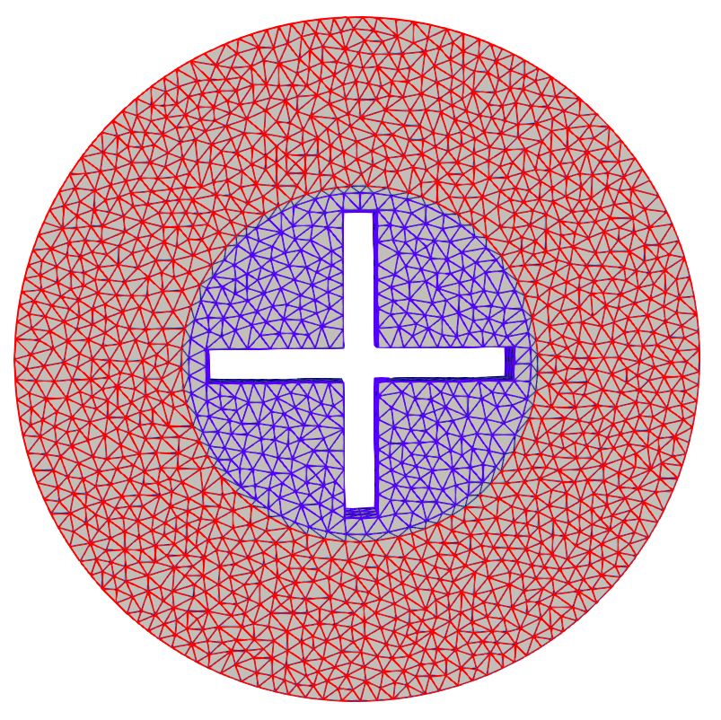
InriaHybrid RANS/VMS 15 3.2 Mesh adaptation for rotating machines Our numerical model has been extended to rotor-stator simulation with a Chimera technique. The Chimera method aims at solving partial differential equations by decomposition into subdomains with overlap in order to avoid having to use a global mesh. This method allows the communication between the computational subdomains thanks to the overlapping of the subdomains. In our case we consider a decomposition in two domains as shown in Fig. 4, a fixed domain in red and a rotating domain in blue. For computations we start by locating the boundary nodes of domain 1 in domain 2, and reciprocally we locate the boundary nodes of domain 2 in domain 1, then the aerodynamic values of each boundary node are determined by interpolation and each domain performs its calculation with the new interpolated values. Figure 4 – Definition of rotor and stator from an initial mesh : in red, the stator, in blue the rotor, and in gray, the overlap region. A mesh adaptation loop based on a metric depending of the Mach number has been combined with the Chimera algorithm. The Transient Fixed Point mesh adaptation algorithm [1, 2, 11] is applied to each domain from a metric field evaluated on the whole domain. RR n° 9464
16                                                                                          Miralles

4     Applications
4.1    Flow past a cylinder
    The predictions of the flow around a circular cylinder are presented. Two Reynolds numbers,
106 and 2×10⁶ , based on the cylinder diameter, D, and on the freestream velocity, are considered.
Only a few numerical investigations have been performed for Reynolds numbers higher than 106 .
This interval is inside the supercritical regime which appears at Reynolds number higher than
2 × 10⁵ and for which the separation becomes turbulent [34].
The computational domain is such that −15 ≤ x, y ≤ 15, and −1 ≤ z ≤ 1 where x, y and z
denote the streamwise, transverse and spanwise directions respectively, the cylinder axis being
located at x = y = z = 0. The mesh contains 4.8 millions nodes.
In order to control the computational costs, a wall law is applied in the close vicinity of the wall.
For accuracy purpose, the Reichardt analytical law [13], which gives a smooth matching between
linear, buffer and logarithmic regions, is chosen. As the y + normalized distance is generally
subject to large variations in complex flows, the wall law is combined with low Reynolds modeling
which locally damps the fully-turbulent model in regions in which the wall law does not cover
the buffer zone.

                               Figure 5 – Computational domain

                                                                                                Inria
Hybrid RANS/VMS 17
Reynolds number 106
The behavior of the hybrid models presented in Section 2 are first investigated in terms of
flow bulk coefficients. From Table ??, it can be noted that the predictions of these coefficients are
globally in good agreement with the experimental data and the numerical results in the literature.
The lift time fluctuations are nevertheless better predicted by the RANS/DVMS model compared
to the other two hybrid models. This good behavior is confirmed by the correct prediction of the
distribution of the mean pressure coefficient, see Fig. 6. On the other hand, it can be observed
from Table ?? and Fig. 6 that Smagorinsky and WALE SGS models give globally comparable
results. It is also worth noting that the RANS model predicts rather well the bulk coefficients.
Fig. 7 shows instantaneous isocontours of the vorticity magnitude for each of the turbulence
models used for this benchmark. As one might expect, the unsteady RANS model is more
dissipative and captures less flow detail than the hybrid models, with in particular a much
more damped and regular wake.
Mesh size +
yw +
ym Cd Cl0 −C pb Lr θ St
Present simulation
RANS k − ε 4.8M 20 100 0.23 0.06 0.23 0.69 132 0.46
DDES k − ε Goldberg 4.8M 20 100 0.20 0.04 0.22 0.87 138 0.13
DDES/ DVMS
k - ε / cubic Smagorinsky 4.8M 20 100 0.20 0.02 0.22 0.82 135 0.42
k - ε / cubic WALE 4.8M 1 100 0.20 0.02 0.26 0.80 132 0.58
RANS / DVMS
k - ε / cubic Smagorinsky 4.8M 20 100 0.24 0.05 0.22 0.62 133 0.42
k - ε / cubic Smagorinsky 4.8M 1 100 0.25 0.09 0.25 0.64 132 0.46
k - ε / cubic WALE 4.8M 1 100 0.26 0.11 0.22 0.65 134 0.42
Other simulations
SRANS Catalano [5] 2.3M - - 0.39 - 0.33 - - -
SLES Catalano [5] 2.3M - - 0.31 - 0.32 - - -
URANS Catalano [5] 2.3M - - 0.40 - 0.41 1.37 - 0.31
LES Kim [18] 6.8M - - 0.27 0.12 0.28 - 108 -
Measurements
Exp. [30] 0.24 - 0.33 - - -
Exp. [29] 0.22 - - - - -
Exp. [35] 0.25 - 0.32 - - -
Exp. [9] - - - - 130 -
Exp. [38] 0.2-0.4 0.1-0.15 0.2-0.34 -
Table 1 – Bulk coefficient of the flow around a circular cylinder at Reynolds number 1M, C d
holds for the mean drag coefficient, Cl0 is the root mean square of lift time fluctuation, C pb is the
pressure coefficient at cylinder basis, Lr is the mean recirculation lenght, θ is the mean separation
angle.
RR n° 946418 Miralles
Figure 6 – Distribution over the cylinder surface of the mean pressure coefficient. Comparaison
between experimental data and numerical results at Reynods 106 .
Figure 7 – Circular cylinder, Reynolds 106 : instantaneous isocontours of the vorticity
magnitude. From top to bottom : RANS, DDES, DDES/DVMS and RANS/DVMS.
InriaHybrid RANS/VMS 19 Figure 8 – Lift and drag coefficient fluctuation. From top to bottom : RANS, DDES, DDES/DVMS and RANS/DVMS. RR n° 9464
20                                                                            Miralles

Figure 9 – Instantaneous vorticity magnitude. From top to bottom : DDES, DDES/DVMS and
RANS/DVMS.

                                                                                  Inria
Hybrid RANS/VMS 21
Reynolds number 2 × 10⁶
The main outputs obtained by the RANS, DDES, DDES/DVMS and RANS/DVMS models
are summed up in Table 2. Regarding the two hybrid models using the DVMS approach, only
the results obtained with the Smagorinsky SGS model are shown, the WALE SGS model giving
very similar results. It can be noticed that all models overpredict the separation angle, and
that the fluctuations of the lift coefficient are overpredicted by the RANS and DDES/DVMS
model. The RANS/DVMS approach gives on the whole the most satisfactory results. In Fig.
10, which shows the distribution of the mean pressure coefficient, the numerical results obtained
with both hybrid models RANS/DVMS and DDES/DVMS are in very good agreement with the
experimental results, in particular RANS/DVMS.
Mesh size +
yw +
ym Cd Cl0 −C pb Lr θ St
Present simulation
RANS k − ε 4.8M 20 100 0.26 0.066 0.30 - 128 -
DDES k − ε Goldberg 4.8M 20 100 0.28 0.038 0.27 - 132 -
DDES/ DVMS
k - ε / cubic Smagorinsky 4.8M 40 100 0.26 0.026 0.35 0.83 130 0.33
k - ε / cubic WALE 4.8M 40 100 0.24 0.020 0.30 1.15 128 0.19
RANS / DVMS
k - ε / cubic Smagorinsky 4.8M 40 100 0.24 0.030 0.30 0.80 132 0.53
k - ε / cubic WALE 4.8M 40 100 0.26 0.057 0.30 0.75 128 0.46
Other simul.
LES/TBLE [33] 0.24 0.029 0.36 - 105
Measurements
Exp. [30] 0.26 0.033 0.40 - 105
Exp. [29] 0.32 0.029 - - -
Table 2 – Bulk coefficient of the flow around a circular cylinder at Reynolds number 2 × 10⁶ .
The subscript S holds for Smagorinsky SGS model.
RR n° 946422 Miralles
Figure 10 – Distribution over the cylinder surface of the mean pressure coefficient. Comparaison
between experimental data and numerical results at Reynods 2 × 10⁶ .
Figure 11 – Lift and drag coefficient fluctuation. From top to bottom : DDES/DVMS and
RANS/DVMS.
InriaHybrid RANS/VMS 23
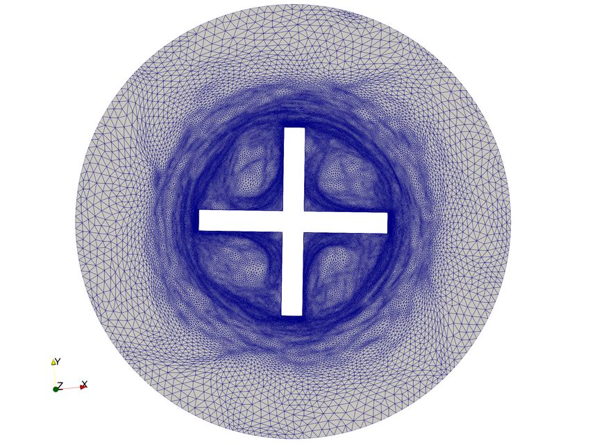
4.2 Flow around a rotating cross
We present a preliminary computation obtained with the combination of the mesh adaptation,
the Chimera approximation and the DDES model. They are used for simulating the mixing
process obtained with the rotation of a cross in a cylindric box. The Reynolds number is 1.8
million, based on the thickness of the blades. The number of vertices of the initial mesh is
10.466. After two turns, and five mesh adaptations, the number of vertices of the adapted mesh
is 1.05 million.
Figure 12 – DDES computation of a rotating mixing device with a mesh adaptative Chimera
approach (horizontal cut). View of the mesh and of Q-factor (colored with velocity magnitude)
after the vertical upper blade.
Figure 13 – DDES computation of a rotating mixing device with a mesh adaptative Chimera
approach (horizontal cut). Partial view of the mesh and velocity magnitude.
In Fig. 12a, we present a view of this final adapted mesh. Mesh size normal to the cylinder
is yet not small enough to allow the creation of strong non-2D features. This is verified from the
examination of the Q-factor, Fig. 12b. Fig. 13 shows details of mesh and velocity magnitude. It
seems from this first calculation that despite the hign Reynold number, the flow separates at
blade angle is a rather stable mode.
5 Conclusion
Several hybrid strategies, based on the DDES, RANS and DVMS models, are first evaluated
for the simulation of the supercritical flow around a circular cylinder. This benchmark is characterized
by turbulent boundary-layer separation. The cylinder flow is first computed at Reynolds 106 . The
predictions of the main flow parameters are in overall good agreement with experimental data
and the results of simulations in the literature, especially the RANS/DVMS model. A second
series of computations of the flow past a circular cylinder is carried out at Reynolds 2 × 10⁶ .
RR n° 946424 Miralles
The predictions obtained by the hybrid models used to perform this benchmark are a little less
accurate compared to the previous Reynolds number, more specifically for the mean separation
angle which is overestimated. Again, the RANS/DVMS model is the hybrid model among those
applied which gives the best results overall. It is also to be noted that the pressure distribution is
well predicted by the hybrid models for both Reynolds numbers, especially by the RANS/DVMS
model. Then, the DDES formulation is applied to the flow around a rotating cross inside a
cylinder with a Reynolds number of 1.8 × 10⁶ . Preliminary results using mesh adaptation with
meshes of 1 million vertices show that separations are more stable than in the flows around the
cylinder. RANS/DVMS computations are planned. The new tool is also being applied to other
rotating devices like propellers and will produce mesh adapted results for these geometries in a
near future.
Acknowledgements
This work was supported by the ANR NORMA project, grant ANR-19-CE40-0020-01 of
the French National Research Agency. The authors gratefully acknowledge GENCI for granted
access to HPC resources through CINES (grants 2020-A0092A05067 and 2021-A0102A06386)
and IDRIS (grant 2021-A0112A05067).
Références
[1] F. Alauzet, P.J. Frey, P.-L. George, and B. Mohammadi. 3D transient fixed point mesh
adaptation for time-dependent problems : Application to CFD simulations. J. Comp. Phys.,
222 :592–623, 2007.
[2] F. Alauzet, A. Loseille, and G. Olivier. Multi-scale anisotropic mesh adaptation for time-
dependent problems. RR-8929, INRIA, June 2016.
[3] P.A. Bakhvalov and T.K. Kozubskaya. On using artificial viscosity in edge-based schemes
on unstructured grids. Mathematical Models and Computer Simulations, 13(4) :705–715,
2021.
[4] S. Camarri, M. V. Salvetti, B. Koobus, and A. Dervieux. A low diffusion muscl scheme for
les on unstructured grids. Comput Fluids, 33 :1101–1129, 2004.
[5] P. Catalano, Meng Wang, G. Iaccarino, and P. Moin. Numerical simulation of the flow
around a circular cylinder at high Reynolds numbers. Int. J. Heat Fluid Flow, 24 :463–469,
2003.
[6] A.P. Duben, T.K. Kozubskaya, P.V. Rodionov, and V.O. Tsvetkova. Ebr schemes with
curvilinear reconstructions of variables in the near-wall region. Computational Mathematics
and mathematical physics, 61(1) :1–16, 2021.
[7] V.A. Garanzha and L.N. Kudryavtseva. Moving deforming mesh generation based on
quasi-isometric functional. Lecture Notes in Computational Science and Engineering, WoS,
Scopus-Q1, 2020.
[8] M. Germano, U. Piomelli, P. Moin, and W. Cabot. A dynamic subgrid-scale eddy viscosity
model. Phys. Fluids A, 3(7) :1760–1765, 1991.
[9] B. Goelling. Experimental investigations of separating boundary-layer flow from circular
cylinder at Reynolds numbers from 105 up to 107 ; three-dimensional vortex flow of a circular
cylinder. In G.E.A. Meier and K.R. Sreenivasan, editors, Proceedings of IUTAM Symposium
on One Hundred Years of Bloundary Layer Research, pages 455–462, The Netherlands, 2006.
Springer.
InriaHybrid RANS/VMS 25
[10] U. Goldberg, O. Peroomian, and S. Chakravarthy. A wall-distance-free k − ε model with
enhanced near-wall treatment. Journal of Fluids Engineering, 120 :457–462, 1998.
[11] D. Guégan, O. Allain, A. Dervieux, and F. Alauzet. An L∞ -Lp mesh adaptive method for
computing unsteady bi-fluid flows. Int. J. Numer. Meth. Eng., 84(11) :1376–1406, 2010.
[12] H. Guillard and C. Viozat. On the behaviour of upwind schemes in the low Mach number
limit. Comput Fluids, 28 :63–86, 1999.
[13] J. Hinze. Turbulence. McGraw-Hil, 1959.
[14] Jens Holmen, Thomas J. R. Hughes, Assad A. Oberai, and Garth N. Wells. Sensitivity of
the scale partition for variational multiscale large-eddy simulation of channel flow. Physics
of Fluids, 16(3) :824–827, 2004.
[15] T.J.R. Hughes, L. Mazzei, and K.E. Jansen. Large eddy simulation and the variational
multiscale method. Comput. Vis. Sci., 3 :47–59, 2000.
[16] E. Itam, S. Wornom, B. Koobus, and A. Dervieux. Combining a ddes model with a
dynamic variational multiscale formulation. In 12th International ERCOFTAC Symposium
on Engineering Turbulence Modelling and Measurements (ETMM12), La Grande Motte,
France, 2018.
[17] Marc Jaeger and Gouri Dhatt. An extended k-epsilon finite element model. International
Journal for Numerical Methods in Fluids, 14(11) :1325–1345, June 1992.
[18] S.-E. Kim and L.S. Mohan. Prediction of unsteady loading on a circular cylinder in
high reynolds number flows using large eddy simulation. Proceedings of OMAE 2005 :
24th International Conference on Offshore Mechanics and Artic Engineering, june 12-16,
Halkidiki, Greece, OMAE 2005-67044, 2005.
[19] B. Koobus and C.. Farhat. A variational multiscale method for the large eddy simulation
of compressible turbulent flows on unstructured meshes-application to vortex shedding.
Comput. Methods Appl. Mech. Eng., 193 :1367–1383, 2004.
[20] Marie-Hélène Lallemand, Hervé Stève, and Alain Dervieux. Unstructured multigridding by
volume agglomeration : Current status. Computers & Fluids, 21 :397–433, 1992.
[21] D.K. Lilly. A proposed modification of the Germano subgrid-scale closure method. Phys.
Fluids, A4 :633, 1992.
[22] R. Martin and H. Guillard. A second-order defect correction scheme for unsteady problems.
Comput Fluids, 25(1) :9–27, 1996.
[23] F. Miralles, B. Sauvage, S. Wornom, B. Koobus, and A. Dervieux. Application of hybrid
RANS/VMS modeling to rotating machines. In Conference on Modelling Fluid Flow
(CMFF’22), The 18th International Conference on Fluid Flow Technologies, Budapest,
Hungary, August 30 -September 2, 2022.
[24] C. Moussaed, M. V. Salvetti, S. Wornom, B. Koobus, and A. Dervieux. Simulation of the
flow past a circular cylinder in the supercritical regime by blending rans and variational-
multiscale les models. Journal of Fluids and Structures, 47 :114–123, 2014.
[25] C. Moussaed, S. Wornom, M.V. Salvetti, B. Koobus, and A. Dervieux. Impact of dynamic
subgrid-scale modeling in variational multiscale large-eddy simulation of bluff body flows.
Acta Mechanica, 225 :3309–3323, 2014.
[26] F. Nicoud and F. Ducros. Subgrid-scale stress modelling based on the square of the velocity
gradient tensor. Flow, Turbulence and Combustion, 62 :183–200, 1999.
[27] H. Reichardt. Vollständige darstellung der turbulenten geschwindigkeitsver-teilung in
glatten leitungen. Zeitschrift für Angewandte Mathematik und Mechanik, 31 :208–219, 1951.
RR n° 946426 Miralles
[28] P.L. Roe. Approximate Riemann solvers parameters vectors and difference schemes. J
Comput Phys, 43 :357–372, 1981.
[29] G. Schewe. On the force fluctuations acting on a circular cylinder in crossflow from
subcritical up to transcritical Reynolds numbers. Journal of Fluid Mechanics, 133 :265–
285, 1995.
[30] W.C.L. Shih, C. Wang, D. Coles, and A. Roshko. Experiments on flow past rough circular
cylinders at large Reynolds numbers. J. Wind Eng. Indust. Aerodyn., 49 :351–368, 1993.
[31] J. Smagorinsky. General circulation experiments with the primitive equations. Monthly
Weather Review, 91(3) :99–164, 1963.
[32] P. R. Spalart, S. Deck, M. L. Shur, K. D. Squires, Strelets M. Kh., and A. K. Travin. A
new version of detached-eddy simulation, resistant to ambiguous grid densities. Theoritical
and Computational Fluid Dynamic, 20(3) :181–195, 2006.
[33] A. Sreenivasan and B. Kannan. Enhanced wall turbulence model for flow over cylinder at
high reynolds number. AIP Advances, 095012, 2019.
[34] B.M. Sumer and J. Fredsoe. Hydrodynamics Around Cylindrical Structures. World Scientific,
2006.
[35] E. Szechenyi. Supercritical Reynolds number simulation for two-dimensional flow over
circular cylinders. J. Fluid Mech., 70 :529–542, 1975.
[36] Hubert Baya Toda, Karine Trun, and Franck Nicoud. Is the dynamic procedure appropriate
for all sgs models. 2010.
[37] B. Van Leer. Towards the ultimate conservative scheme. iv : a new approach to numerical
convection. J Comput Phys, 23 :276–299, 1977.
[38] M. M. Zdravkovich. Different modes on vortex shedding : an overview. Journal of Fluid
and Structures, 10(5) :427–437, 1996.
InriaRESEARCH CENTRE Publisher
SOPHIA ANTIPOLIS – MÉDITERRANÉE Inria
Domaine de Voluceau - Rocquencourt
2004 route des Lucioles - BP 93 BP 105 - 78153 Le Chesnay Cedex
06902 Sophia Antipolis Cedex inria.fr
ISSN 0249-6399You can also read