DISCUSSION PAPER SERIES - Sunset Long Shadows: Time, Crime, and Perception of Change
←
→
Page content transcription
If your browser does not render page correctly, please read the page content below
DISCUSSION PAPER SERIES

IZA DP No. 14770

Sunset Long Shadows:
Time, Crime, and Perception of Change

Pavel Jelnov

OCTOBER 2021
DISCUSSION PAPER SERIES

IZA DP No. 14770

Sunset Long Shadows:
Time, Crime, and Perception of Change

Pavel Jelnov
Leibniz Universität Hannover and IZA

OCTOBER 2021

Any opinions expressed in this paper are those of the author(s) and not those of IZA. Research published in this series may
include views on policy, but IZA takes no institutional policy positions. The IZA research network is committed to the IZA
Guiding Principles of Research Integrity.
The IZA Institute of Labor Economics is an independent economic research institute that conducts research in labor economics
and offers evidence-based policy advice on labor market issues. Supported by the Deutsche Post Foundation, IZA runs the
world’s largest network of economists, whose research aims to provide answers to the global labor market challenges of our
time. Our key objective is to build bridges between academic research, policymakers and society.
IZA Discussion Papers often represent preliminary work and are circulated to encourage discussion. Citation of such a paper
should account for its provisional character. A revised version may be available directly from the author.

                                                     ISSN: 2365-9793

                                           IZA – Institute of Labor Economics
Schaumburg-Lippe-Straße 5–9                      Phone: +49-228-3894-0
53113 Bonn, Germany                             Email: publications@iza.org                                    www.iza.org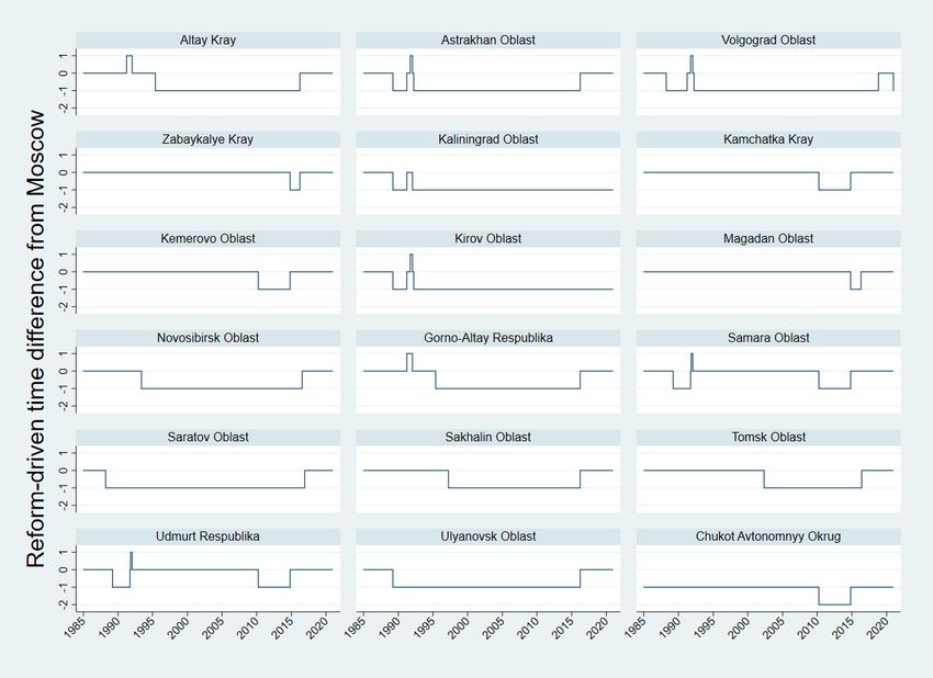
IZA DP No. 14770                                                                                        OCTOBER 2021

            ABSTRACT
            Sunset Long Shadows:
            Time, Crime, and Perception of Change
            How long survives perception of change after evaporation of the actual change? I
            investigate the effect of daylight on crime and fear of crime. Forty years of reforms shifted
            the boundaries between Russian eleven time zones. I find that a permanent switch to a
            later sunset leads to a two year long decrease in robbery and has no effect on homicide.
            The magnitude of the effect on robbery is similar to the previous estimates from other
            countries immediately after daylight saving time transitions. Even though the actual effect
            lasts two years, women report in a 10-year perspective increased feeling of safety even
            in darkness. However, men report increased feeling of safety only as long as the actual
            decrease in robbery persists.

            JEL Classification:        J18
            Keywords:                  crime, daylight saving time, fear of crime, homicide, robbery,
                                       Russia, time zones

            Corresponding author:
            Pavel Jelnov
            Wirtschaftswissenschaftliche Fakultät
            Institut für Arbeitsökonomik
            Leibniz Universität Hannover
            Königsworther Platz 1
            30167 Hannover
            Germany
            E-mail: jelnov@aoek.uni-hannover.de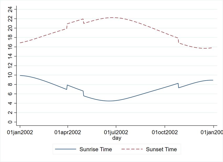
1     Introduction
The ongoing climate and Covid-19 crises refreshed our understanding that despite industrial-
ization, humans depend on nature. There is increasing interest in how environmental factors
affect economics (Burke et al., 2015, Cole et al., 2017, Dell et al., 2014, Deschênes and Green-
stone, 2011, Dillender, 2021, Hajdu and Hajdu, 2021, Jessoe et al., 2018, de Oliveira et al.,
2021). One of the most important natural resources is daylight. Yet modern institutions that
accommodate society to daylight, i.e., time zones and daylight saving time (DST), remain
variable and their efficiency remains, more than a century after their introduction, uncertain.
For instance, recently, the European Union relied on a poll in a decision to abolish DST
transitions. This decision set a dilemma in front of each EU member to which time zone it
shall belong.
     In this paper, I investigate the effect of daylight on crime and fear of crime. I study the
case of Russia, the biggest time laboratory in the world, which has eleven time zones and
exercises frequent reforms that shift their boundaries. I employ official records to assess the
effect of time reforms on crime and use longitudinal survey data to assess the effect of the
reforms on fear of crime and on the related behavior.
     The paper touches three issues: the optimal regional time zone, the divergence between
actual crime and crime perception, and the long-run effects of ambient light on crime and
behavior. Hence, the paper makes several contributions. First, to the best of my knowledge,
it is the first use of a natural experiment to assess not only the immediate but also the long
run effect of daylight on crime. Previous studies estimated the regression discontinuity at
DST transitions, which is, by the seasonal design of DST, cancelled out in the long run.
Contrary, I consider permanent changes and their long-run effect.1
     The second contribution is to a discussion on divergence between crime and its perception.
To this end, I utilize a longitudinal survey that inquires about respondent’s feeling safe to
walk in darkness. Even though no time reform can change the nature of darkness, I find
a strong permanent effect of time reforms on the perceived safety indicator. Finally, the
paper contributes to the literature on the interaction between environment and society. In
  1
   Bünnings and Schiele (2021) analyze the permanent effect of daylight on traffic accidents in the United
Kingdom.

                                                  2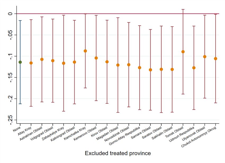
particular, the fit between the natural and the social schedules has long been investigated in
the medical literature and has recently received growing attention from economists.
    My empirical analysis is divided into two parts. In the first part, I estimate the effect
of time reforms on crime. In line with most previous literature, I focus on robbery, the
most relevant crime in the context of outside meetings between offenders and victims. I also
analyze homicide. For identification, I apply the lags-and-leads model (Hajdu and Hajdu,
2021) and check the robustness of the results using the Borusyak et al. (2021) method for
event analysis.
    I document a decrease of around 11% in robbery in the first year after a shift to a higher
time zone, i.e., one-hour later sunset, and a decrease of around 13% two years after the reform.
This result is almost equal to the recent estimates of the immediate DST transition effect
in Uruguay, provided in Tealde (2021), who follows Domínguez and Asahi (2019), Munyo
(2018), Umbach et al. (2017), Toro et al. (2016), Doleac and Sanders (2015), and Toro et al.
(2015) in investigation of the effect of DST transitions on crime in the western hemisphere.
Therefore, I document that the immediate effect, documented in the previous literature for
DST transitions, can be observed for two years if the transition is permanent. However, I
find no effect on homicide.
    In the second part of the analysis, I confront the actual effect on crime with its perception
by individuals. Even though the effect on robbery persists for two years and there is no
effect on homicide, I find that the behavioral effect of time reforms is strong and permanent.
Analysis of longitudinal survey data shows that in a 10-year perspective women are still more
likely to report feeling safe to walk in darkness in their neighborhood of residence. The effect
on men lasts only two years, similarly to the effect on actual robbery. The results are similar
in European and Asian regions of Russia.
    Not only the reported fear is affected but also the actual behavior. I find that following
the reforms, individuals increase their walking for daily needs. This result is related to the
causal effect of crime on walking, documented in Janke et al. (2016) and is in line with
findings on the positive effect of DST on outdoor activity, found in Wolff and Makino (2012).
I also investigate the effect on sleep and find a two-year decrease in sleep, correspondingly to
the literature that studies sleep in the context of time use (Giuntella and Mazzonna, 2019,
Umbach et al., 2017, Hamermesh et al., 2008). The decrease in sleep indicates a shift toward

                                               3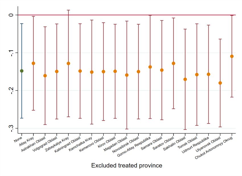
other activities, which may be related to the enhanced feeling of safety to spend time outside.
     The effect of daylight on crime and fear of crime is nested in the literature on the inter-
action between physical environment and humans (Triguero-Mas et al., 2015). For instance,
heat and large variations in climate are associated with a higher incidence of crime and con-
flict (Baysan et al., 2019, Ranson, 2014). The effect of weather on aggression is combined
of the direct effect of heat, sunlight, humidity, etc., on mood and the indirect effect through
economy, outside activity, and social interaction (Keller et al., 2005). Daylight directly af-
fects human physiology and psychology through vision, skin, and nonvisual ocular actions
on the circadian clock in the brain and on other neuronal pathways (Münch et al., 2017). It
mitigates seasonal affective disorder (SAD), depression with typical onset during the fall or
winter and remission in the spring (Azmitia, 2020, Kurlansik and Ibay, 2012, Keller et al.,
2005). The emotional effects of light may include not only decreased aggression but also de-
creased fear (Kawamura et al., 2019, Yoshiike et al., 2018, Warthen et al., 2011). Therefore,
both the actual crime and fear of it should be assessed as separate outcomes.
     In addition, a body of research documents that light, sun, clear air, and good weather con-
tribute to honest and pro-social behavior (Lu et al., 2018, Guéguen and Jacob, 2014, Guéguen
and Stefan, 2013, Guéguen and Lamy, 2013, Zhong et al., 2010, Rind and Strohmetz, 2001,
Rind, 1996). Experimental evidence shows that improved street lighting is associated with a
lower crime rate (Tealde, 2021, Chalfin et al., 2019, Arvate et al., 2018, Welsh and Farrington,
2008), and improved lighting at sport facilities leads to decreased violence (Amorim et al.,
2016). These effects may be related not only to the increased probability of arrest and pun-
ishment when the crime is committed in light (Tealde, 2021) but also to decreased aggression.
Related socio-ecological mechanisms were found also in the effect of the landscape and land
use of public spaces on crime and fear of crime (Rišová and Madajová, 2020, Mak and Jim,
2018, Twinam, 2017, Tandogan and Ilhan, 2016, Sreetheran and Van Den Bosch, 2014) and
in the difference between police behavior in light and darkness (Horrace and Rohlin, 2016).
     Finally, the economic context of this paper is the social cost of crime. Exploration of
incentives to commit crime dates back to Becker (1968), while discussion and estimates of
the social cost of crime can be found in Koppensteiner and Menezes (2021), Ponomarenko
and Friedman (2017), Welsh et al. (2015), Wickramasekera et al. (2015), Anderson et al.
(2012), Heaton (2010), McCollister et al. (2010), and Ayres and Levitt (1998). Recently,

                                               4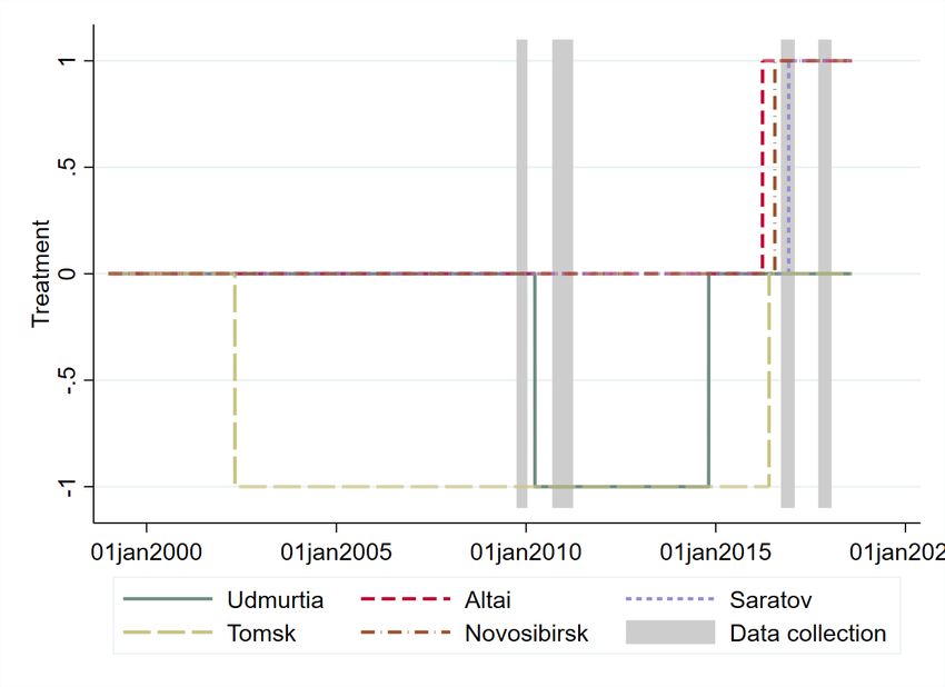
Velásquez (2020) and earlier Dell (2015) document the negative effect of Mexican drug war
on the weak segment of the labor force, i.e., female and informal sector workers. From
behavioral perspective, Becker and Rubinstein (2011) provide a conceptual framework and
empirical evidence that fear of terrorism is endogenous to the individual economic activity.
Fear of crime is addressed in Janke et al. (2016), Stearns (2012), Czabanski (2008), Dolan
and Peasgood (2007), and Moore and Shepherd (2006).
The paper proceeds as follows. Section 2 addresses the history of Russian time zone
reforms. In Section 3, I use province-level crime records to investigate the effect of time
reforms on crime, and in Section 4, I utilize a longitudinal survey to assess the effect of the
reforms on fear of crime, walking, and sleep. Section 5 concludes.
2 Background
Russia is an exceptional case to study the effects of environmental variables. It uniquely
combines vast geography with a relatively homogeneous population, 80% of which are ethnic
Russians. The Soviet government imposed geographic redistribution of population alongside
cultural equalization. As a result, the Soviet heritage is a large but culturally homogeneous
country, where ethnic Russians are the major group in most regions, and minorities are
mostly concentrated in a few “national republics” and in the far north. The combination of
diverse geography and homogeneous population enhances identification of the causal effects
of environmental variables on socio-economic indicators.
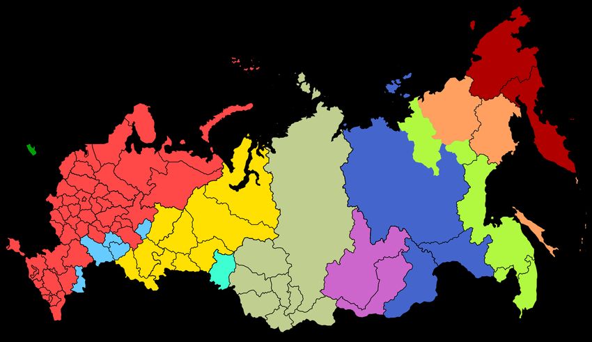
The longitudinal distance between Russian westernmost province,2 Kaliningrad, and the
easternmost province, Chukotka, is 157 , corresponding to 11 natural (nautical) time zones.
Russia indeed has eleven time zones, shown on the map in Figure A.1 in Appendix. A
natural time zone is the one that places the sun in the zenith around 12pm. However, the
Russian time zones are not natural in this sense in most of the regions. For instance, in
the period between 1990 and 2015, the time was equal to the natural one in only 196 out of
2,162 province-year cases. Between 1995 and 2014, the number was only 20 out of 1,662. In
almost all of the other cases, institutional time exceeds the natural time. Between 1990 and
2
The official Russian term for a province is “federal subject”.
52015, institutional time exceeded the natural time by one hour in 52% of the province-year
cases, and by two hours in 38% of the cases. It means that sunrise and sunset in Russia are,
roughly speaking, institutionally late.
Russia differs from other countries by its frequent time reforms. The time zones were
introduced in 1919 and were expanded to the whole territory of the Soviet Union in 1924.
The introduction of the time zones was followed by a long list of changes that continue to
this day. In particular, the difficulty to manage eleven time zones led Russia to experience
19 time reforms since 1980. In addition to the reforms that shifted the time zone boundaries,
Russia observed DST from 1981 to 2011. To illustrate these time changes, Figure 1 shows
the sunrise and sunset times in 2002 in the Siberian city of Tomsk. The figure exhibits three
discontinuities. The first discontinuity is the DST transition in March, common to entire
Russia. The second discontinuity is the reform that took place in May, affected only Tomsk,
and set its clocks back by one hour. The third discontinuity is the October shift back from
DST.
The frequency of time reforms has been particularly high since the late 1980s, before
and after the collapse of the Soviet Union. Time zones affect coordination between regions
(Christen, 2017, Hattari and Rajan, 2012, Hamermesh et al., 2008, Stein and Daude, 2007,
Kikuchi et al., 2006), but Russian time reforms are related to a more general struggle between
the country’s vast geography and political centralization.3
In particular, about 50 out of the total4 of 85 provinces use Moscow Time. The 2010–2018
cycle of reforms illustrates its dominance but shows also the resistance to time coordination
with Moscow. The president stated in 2009 that distant regions should be set “closer” to
Moscow, which should improve the coordination between the local governments and the
central one. In the following year, the number of time zones shrank from eleven to nine
(by changing the time in five provinces), and the number of provinces in the Moscow Time
zone increased from 50 to 52 and increased further to 54 in 2014 after annexation of Crimea.
3
In some countries, time is being manipulated not only for political but even for symbolic reasons, e.g.,
in revolutionary China, Francoist Spain, Chávez-led Venezuela, and North Korea. In China, the tension
between forced centralization and nature created the anomaly of Xinjiang time, where two times with a two-
hour difference are used in the same province, and the separation lies along ethnic rather than geographic
lines.
4
Including Crimea and Sevastopol, annexed in 2014. The annexation is not recognized internationally.
6However, the implementation of the 2010 reform was unpopular. The reform was recognized
as a failure already in 2011, leading to another reform. The third reform, in 2014, restored the
two missing time zones. Furthermore, ten provinces changed their time in 2016, an additional
province changed it in 2018 but returned to the former time in 2020. This cycle of reforms
exhibits the unresolved trade-off between nature and centralization.
As a result, while some reforms, such as introduction of the DST in 1981 and its abolition
in 2011, affect the entire country, many reforms involve only specific regions. Table 1 lists
all the reforms that took place since 1980. The table indicates the number of the affected
provinces and shows the direction of each change.5
Throughout the paper, I use the following definition:
“Treatment” is a change in time difference from Moscow.
This definition of treatment is equivalent to the sunrise or sunset times stripped from the
location, year, and day of the year fixed effects. The location fixed effects control for the
mean time at the location. The year fixed effects control for any time changes common to all
of the country, e.g., DST transitions (which keep time difference from Moscow unchanged).
Finally, the day of the year fixed effects control for the curve of sunrise and sunset times
over the year. Because the day fixed effects absorb any seasonal fluctuations in the daylight
duration at a given location, the sunrise and sunset times are fully correlated in presence of
the location and day fixed effects. Therefore, time difference from Moscow fully absorbs any
reform-driven fluctuations in the sunrise and sunset times.
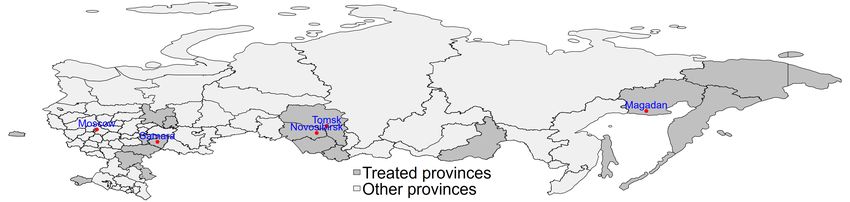
There are 18 provinces that satisfy this definition. Figure 2 shows the map of Russia,
where the treated provinces are shadowed. Figure 3 follows the reform-driven changes in
time difference from Moscow in these provinces.
The largest (in terms of population) group of treated provinces covers the banks of Volga
river, close to the boundary between European and Asian parts of Russia. This is where the
vast Moscow Time zone ends. Because of the dominance of Moscow Time (UTC+3), the
Samara Time (UTC+4), which runs along Volga, covers a relatively small region. Struggling
to exist, the Samara Time zone experienced several changes to its boundaries between 1988
5
Because I use crime records from 1990 on and consider the 10-year lag of time reforms, 1980 is the first
year entering this paper’s analysis.
7and 1992, was completely extinct between 2010 and 2014, included only two provinces in
2014, was expanded to five provinces in 2016, to six provinces in 2018 and shrank back to
five provinces in 2020.
The second region that is subject to relatively frequent reforms includes provinces in
the orbit of the strong city of Novosibirsk in Western Siberia. Between 1991 and 2002 and
in 2016, different provinces in this region experienced time changes. For instance, the 1995
reform in Altai and the 2002 reform in Tomsk followed the 1993 reform in Novosibirsk, partly
because many workers travel frequently between Altai, Tomsk, and Novosibirsk, and time
coordination with Novosibirsk synchronizes the train schedule.
In addition, the map in Figures 2 indicates that special reforms involved also the far east
of Russia as well as its westernmost province, Kaliningrad. Not surprisingly, the trade-off
between centralization and nature is salient in the western and eastern periphery of the vast
country. Finally, following its internationally unrecognized annexation by Russia in 2014,
also Crimea became a “treated” region when it set its clocks by two hours forward to align
with Moscow Time. Yet I exclude Crimea from the analysis, because it was not incorporated
in Russia until 2014.
3 Time Reforms Effect on Crime
Data
I use the annual reports “Regions of Russia: Socioeconomic Outcomes” published by the
Federal State Statistics Service (Rosstat). The annual reports cover a wide range of topics,
aggregated on provincial level. The first report is from 2002 but it includes data also for
1990, 1995, and from 1998 on. I exclude Crimea and Sevastopol, annexed in 2014, and the
remaining sample consists of 83 provinces. The incidence of robbery appears in this data for
the 2001–2018 period, while the incidence of homicide appears for the 1990–2018 period.
Table 2 presents the summary statistics, separately for untreated and treated provinces.
The treated are 16 provinces that experienced a change in time difference from Moscow
during the 2001–2018 period, for which I have robbery data (Kirov and Kaliningrad, shown in
Figure 3, experienced such a change before 2001). The variables in the table are homicide and
8Figure 1: Sunrise and sunset times in Tomsk in 2002
Note: The figure shows the sunrise and sunset times in Tomsk, a province capital in Western Siberia, in 2002. The discontinuities
are, in chronological order, the transition to DST, common to all Russia, a time reform, special to Tomsk, and the transition
back from DST.
Figure 2: Treated provinces
Note: The figure shows the provinces that experienced a change in time difference from Moscow since 1980. The evolution of
time difference from Moscow in these provinces is shown in Figure 3. The map includes Crimea, annexed by Russia in March
2014. The annexation is not recognized internationally.
9Figure 3: Change in time difference from Moscow in the treated provinces
Note: The figure shows change in time difference from Moscow in the treated provinces.
10Table 1: Russian time reforms
Date Affected provinces Direction Remarks
April 1, 1981 All " First DST transition
April 1, 1982 Chukotka #
March 27, 1988 Volgograd, Saratov #
March 26, 1989 6 provinces #
March 31, 1991 78 provinces #
October 30, 1991 Samara, Udmurtia "
January 19, 1992 75 provinces "
March 29, 1992 Astrakhan, Volgograd #
May 23, 1993 Novosibirsk #
May 28, 1995 Altai Krai, Altai Republic #
March 30, 1997 Sakhalin #
May 1, 2002 Tomsk #
March 28, 2010 5 provinces # The number of time zones decreases to 9
August 31, 2011 All " Elimination of DST
March 30, 2014 Crimea, Sevastopol *
October 26, 2014 80 provinces # (78 provinces) + (2 provinces) Restoration of 11 time zones
March 27 to December 4, 2016 10 provinces "
October 28, 2018 Volgograd "
December 27, 2020 Volgograd #
Note: The table lists time reforms in Russia since 1980. The signs " and # correspond to a shift of one hour, while * and +
correspond to a shift of two hours. The number of affected provinces is given in accordance with the administrative division of
Russia in 2020. Crimea was annexed by Russia in March 2014, but the annexation is not recognized internationally.
11Table 2: Summary statistics of provincial data
Variable Mean Std. Dev. Obs. Mean Std. Dev. Obs. Years
Untreated provinces Treated provinces
ln (Homicide rate) 2.614 0.623 1,613 2.779 0.568 448 1990–2018
ln (Robbery rate) 4.225 1.020 1,170 4.549 0.694 324 2001–2018
ln (Alcohol sales) 1.945 0.695 1,304 2.069 0.344 378 1998–20018
ln (Personal income) 8.436 2.365 1,662 8.482 2.320 466 1990–2019
ln (GDP per capita) 11.356 1.419 1,502 11.477 1.361 432 1995–2018
ln (Population) 7.162 0.897 1,625 6.877 1.103 450 1990–2018
ln (Academic graduates rate) 1.561 0.691 1,580 1.644 0.593 428 1990–2018
ln (Restauran visits per capita) 0.356 2.497 1,361 0.436 2.431 378 1990–2018
Share of working-age population 0.594 0.036 1,690 0.609 0.041 468 1990–2019
Sex ratio 0.876 0.045 1,690 0.902 0.060 468 1990–2019
Note: The table presents summary statistics of province-level annual records of socio-economic indicators. Alcohol is per-capita
annual sales of pure alcohol in liters, calculated from Rosstat data on alcohol sales. In order to calculate the pure alcohol, I
weight the sales of different beverages by their alcohol content: 0.4 for vodka and cognac, 0.12 for wine and sparkling wine, and
0.05 for beer. Source of data: Rosstat “Regions of Russia“ annual reports.
robbery rates per 100,000 of population, pure alcohol sales per capita, mean personal income
and GDP per capita, rate of new academic graduates per 1,000 of population, restaurant
visits per capita, share of population in working age,6 and the sex ratio. The summary
statistics show that the treated provinces are slightly more developed in terms of income and
education but have higher homicide and robbery rates.
Baseline estimation
I start with a two-way fixed effects model, where the explanatory variables are leads and lags
of time difference from Moscow. A similar model can be found in Hajdu and Hajdu (2021),
who investigate the effect of temperature on fertility. For implementation of this approach
with annual data, the treatment variable is averaged over the calendar year:
6
Working age is 16–59 for men and 16–54 for women.
12365
X
T̄iy = Tity (1)
t=1
where T is time difference from Moscow in province (or location in individual data in
Section 4) i on date t of year y.
The econometric model includes n leads and 10 lags of T :
n
X
ln(ciy ) = k T̄i,y+k + i + y + Xiy µ + "iy (2)
k= 10
where c is the crime indicator (robbery or homicide rate per 100,000 of population). The
fixed effects are i for the province and y for the year. The residuals "iy are clustered on
the provincial level. Xiy is a vector of control variables, which includes logged mean personal
income and its square and logged GDP per capita and its square.
Note that this model is not a canonical “event study”. The explanatory variables are
the leads and lags of time difference from Moscow and not the dummies for the number
of years until/since treatment. As Section 2 discusses and Table 1 and Figure 3 show, the
multiple time reforms generate complex changes in time difference from Moscow. These
changes are not simple "from 0 to 1" events. Some treated provinces shift the time up on
some reforms and shift it down on other reforms. Therefore, the empirical setup here is not
the canonical “staggered rollout” story, when the same treatment is given to different panel
units in different years. Yet as a robustness check below, I limit the sample to provinces that
experience a single monotonic change in time difference from Moscow, such that the setup
fits the “staggered rollout” definition, and apply the Borusyak et al. (2021) robust estimator
for event studies.
Back to the model in Equation (2), the number of leads is n. The role of the leads is to
test for the correlation of the current outcome with future treatment. There is a trade-off
between the number of leads and the sample size: leads erase the last years in data, because
for these years the future time difference from Moscow is not yet known. In order to lose no
data, I estimate the model with three leads at most.
Table 3 presents the estimation results for n=1, 2, and 3 for logs of robbery (columns
1–3) and homicide (columns 4–6) rates. The results show that leads are not related to the
13current robbery rate. In terms of identification, future reforms are not correlated with the
current outcome. The most important results are the coefficients of lags. The first lag has
a -0.114 log points effect (10.8%) on robbery when n=3 (-0.12 log points when n=1). The
second lag has a -0.142 log points effect (13.2%) on robbery when n=3 (-0.129 log points when
n=1). Both lags are statistically significant. From the third lag on, there is no statistically
significant effect of past time reforms on robbery.
These results can be compared to the existing estimates from regression discontinuity
studies that use DST transitions and explore their immediate effect on robbery. Tealde
(2021) finds a decrease of 17% in robbery in Uruguay, Doleac and Sanders (2015) find a
7% effect in the U.S., Domínguez and Asahi (2019) document a reduction of 20% in major
Chilean cities, and Munyo (2018) finds a 24% decrease in Montevideo. Therefore, my results
fall in the range of existing estimates from regression discontinuity studies. However, my
paper is the first one to show that the effect may persist for two years if the time shift is
permanent.
I find no effect of time reforms on homicide (columns 4–6). The difference in the results
for robbery and homicide is supportive evidence that the estimated coefficients are indeed
the causal effect of time reforms. Plausibly, the effect on robbery should be stronger than on
homicide. Robbery is more likely than homicide to be a result of random outside meetings
between offenders and victims, and, therefore, is more sensitive to environmental conditions,
such as ambient light. The fact that the results are different for robbery and homicide implies
that the first and second lag effects on robbery are not a result of general crime trends in
the treated provinces, correlated but not implied by time reforms.
Robustness checks and alternative models
Sensitivity analysis
I perform a set of sensitivity and robustness checks of the baseline results. First, I consider
the sensitivity of the time reforms effect to exclusion from the sample of any treated province.
Figure A.2 in the Appendix shows the first lag coefficient, when I estimate Equation (2) and
exclude the 18 treated provinces one by one. Similarly, Figure A.3 shows the sensitivity of the
second lag coefficient. The first bar in each figure depicts the coefficient in the full sample andTable 3: Time reforms effect on robbery and homicide rates
Robbery Robbery Robbery Homicide Homicide Homicide
(1) (2) (3) (4) (5) (6)
Time (+3) -0.0144 -0.0722
(0.0834) (0.0703)
Time (+2) -0.0904 -0.0751 -0.0301 0.0465
(0.0981) (0.0752) (0.0567) (0.0588)
Time (+1) -0.103 -0.00432 -0.00955 -0.0178 0.0135 -0.00983
(0.0850) (0.0836) (0.0702) (0.0546) (0.0539) (0.0534)
Time -0.0140 -0.0419 -0.0396 0.0130 0.00521 0.0147
(0.0523) (0.0558) (0.0514) (0.0395) (0.0366) (0.0392)
Time ( 1) -0.120** -0.113** -0.114** 0.0126 0.0149 0.00947
(0.0510) (0.0525) (0.0495) (0.0387) (0.0364) (0.0375)
Time ( 2) -0.129* -0.139* -0.142** -0.00967 -0.0129 -0.0230
(0.0724) (0.0712) (0.0697) (0.0471) (0.0463) (0.0479)
Time ( 3) 0.0292 -0.0105 -0.00554 0.0318 0.0263 0.0407
(0.101) (0.114) (0.116) (0.0604) (0.0635) (0.0668)
Time ( 4) -0.0141 0.0677 0.0624 -0.0484 -0.0403 -0.0471
(0.131) (0.149) (0.139) (0.0855) (0.0875) (0.0897)
Time ( 5) -0.129 -0.187 -0.184 0.0110 0.00818 0.0102
(0.171) (0.135) (0.146) (0.0332) (0.0319) (0.0314)
Time ( 6) 0.0702 0.0875 0.0852 -0.0310 -0.0307 -0.0344
(0.134) (0.126) (0.132) (0.0580) (0.0579) (0.0587)
Time ( 7) -0.0684 -0.0825 -0.0826 -0.0206 -0.0223 -0.0227
(0.0984) (0.106) (0.106) (0.0375) (0.0375) (0.0377)
Time ( 8) 0.0299 0.0210 0.0234 -0.0267 -0.0278 -0.0268
(0.126) (0.122) (0.130) (0.0193) (0.0189) (0.0191)
Time ( 9) -0.0431 -0.0274 -0.0297 0.00232 0.00296 0.00168
(0.199) (0.192) (0.200) (0.0480) (0.0474) (0.0479)
Time ( 10) -0.0512 -0.0632 -0.0644 -0.0330 -0.0351 -0.0403
(0.112) (0.107) (0.104) (0.0492) (0.0469) (0.0453)
Controls Yes Yes Yes Yes Yes Yes
Year FE Yes Yes Yes Yes Yes Yes
Province FE Yes Yes Yes Yes Yes Yes
Observations 1,455 1,455 1,455 1,929 1,929 1,929
Number of provinces 83 83 83 83 83 83
Notes: The table presents the results of estimation of Equation (2) with standard errors clustered on province level. Time is
time difference from Moscow. Control variables include log of GDP per capita, its square, log of mean personal income, and
its square. The dependent variables are log of annual robbery and homicide cases per 100,000 of population. *** pcorresponds to the baseline results in column 3 of Table 3. Other bars show the coefficient
when one treated province is excluded from the sample. The conclusion from the graphs is
that exclusion of no province erases the treatment effect one and two years after treatment.
The magnitude of the first lag is always around -0.1 log points, and the magnitude of the
second lag is always between -0.1 and -0.2 log points. This sensitivity analysis is important for
the exclusion restriction: the sign and the magnitude of the coefficients is robust to exclusion
of any treated province. Therefore, the treatment effect on robbery is not driven by any local
trend correlated with treatment.
Effect monotonicity
Second, I address the fact that some reforms shifted the time in some provinces by two
hours. This feature of Russian time reforms may be used to test for monotonicity of their
effect. The question here is whether the effect of a two-hour shift has the same sign and
is stronger than that of a one-hour shift. I round the average annual time difference from
Moscow and estimate a model where the treatment variables are a set of dummies for the
rounded reform-driven time difference from Moscow.
The model is
ln(ciy ) = ↵1 Tiy1 + ↵2 Tiy2 + ˆi + ˆy + Xiy µ̂ + "ˆiy (3)
where T1 and T2 are, respectively, dummy variables for one-hour and two-hour time
differences from Moscow (after rounding).
Table 4 shows the results for robbery and homicide. A one-hour change in time difference
from Moscow is associated with a 0.21–0.23 log points decrease in robbery rate (column
1 without controls, column 2 with controls), while a two-hour change is associated with a
0.32–0.34 log points decrease. Again, there is no effect on homicide (columns 3 and 4).
Event analysis
Finally, I challenge the baseline two-way fixed effects model. The recent boost in econometric
theory revises the common practice of difference-in-differences estimation of treatment effects
16Table 4: Time reforms effect on robbery and homicide rates: ordinal treatment variable
Robbery Robbery Homicide Homicide
(1) (2) (3) (4)
Treatment = 1 -0.230*** -0.210*** 0.009 0.019
(0.078) (0.078) (0.053) (0.048)
Treatment = 2 -0.342*** -0.322*** 0.014 0.047
(0.108) (0.110) (0.091) (0.101)
Controls No Yes No Yes
Year FE Yes Yes Yes Yes
Province FE Yes Yes Yes Yes
Observations 1,494 1,455 2,061 1,929
Number of provinces 83 83 83 83
Notes: The table presents the results of estimation of Equation (3) with standard errors clustered on province level. Treatment
are two dummy variables, indicating the values of a rounded time difference from Moscow. Control variables include log of GDP
per capita, its square, log of mean personal income, and its square. The dependent variables are log of annual robbery and
homicide cases per 100,000 of population. *** p(Athey and Imbens, 2021; Borusyak et al., 2021; Callaway and Sant’Anna, 2020; De Chaise-
martin and d’Haultfoeuille, 2020; Goodman-Bacon, 2021; Sun and Abraham, 2020). This
literature points out that the problem with the difference-in-differences approach when treat-
ment is given to different panel units at different time is that units treated early serve as
control units for those treated later. The early-treated units are affected by treatment, and,
therefore, are not proper control units. The difference-in-differences estimator is a weighted
mean of outcome differences between all pairs of units (Goodman-Bacon, 2021). The differ-
ences between early-treated and later-treated units may have negative weights, leading to a
bias of the estimated treatment effect. The above-mentioned recent studies propose different
alternative estimators that should correct the bias.
The setup that I analyze falls in the category of cases that this literature addresses,
because of the multiple time reforms. However, the problem is not acute: only 16 out of 83
provinces experience variation in time difference from Moscow during the 2001–2018 period,
for which I hold the robbery data. Therefore, vast majority of comparisons are between
treated and never-treated units, and only a small number of comparisons is between later-
treated and earlier-treated units. Yet I test the robustness of the two-way fixed effect model
by applying the Borusyak et al. (2021) estimator for event studies. This estimator is the
most recent contribution that outperforms the solutions proposed in De Chaisemartin and
d’Haultfoeuille (2020), Sun and Abraham (2020), and Callaway and Sant’Anna (2020), and
is a unique efficient linear unbiased estimator under some assumptions. The estimator is
currently implemented for settings with a binary monotonic treatment status, where in each
period treatment can either switch from zero to one or remain zero. Therefore, I exclude
from the sample eight provinces with non-monotonic time difference from Moscow during the
2001–2018 period. The remaining data consists of 75 provinces, eight if which are treated.
The event is a shift to a one-hour later time. All these reforms took place in the 2016–2018
period, while my data ends in 2018, such that I can only test for the reform effect up to two
years forward. I can now apply the Borusyak et al. (2021) estimator (hereafter BJS) for the
event study model, where the explanatory variables are dummies for the number of years
until/since the event:
182
X
ln(ciy ) = ⌧k [Kiy = h] + ˜i + ˜y + "˜iy (4)
h= m
where K is the number of years since the event. Table 5 presents the results for m= 3, 4,
and 5. The BJS estimator confirms the baseline results: a one-hour-forward time shift leads
to a 0.101 (10.6%) log points decrease in robbery in a one-year and to a 0.189 log points
(20.8%) decrease in a two-year perspective. The latter effect is statistically significant. The
coefficient for the second lag is slightly higher than in the baseline estimation, suggesting
that the negative weights problem in the difference-in-differences model indeed generated
some toward-zero bias. However, this bias is not large, consistently with being the number
of “forbidden comparisons” (comparisons with a negative weight) in the full data set small.
4 Time Reforms Effect on Fear of Crime
Data
For assessment of fear of crime and related behavioral outcomes, I utilize the Russian Lon-
gitudinal Monitoring Survey (RLMS) by Higher School of Economics (1994–2019). It is the
main if not the only data set to be used for investigation of individual and household out-
comes across Russia. The participants are individuals from 161 settlements in 40 locations in
33 provinces. So far, RLMS collected 372,000 individual and 138,000 household observations.
The overall number of individuals that have been investigated is 57,000, of whom 45,000 were
at least 18 years old at the time of at least one interview. Data is always collected between
September and March, and in most of the waves it is collected between October and Decem-
ber. I restrict the sample to respondents at least 18 years old. For the purpose of clustering
the standard errors by settlement, I exclude the few individuals who moved between RLMS
settlements during the survey.
The map in Figure 4 shows the 40 locations. Empty circles indicate the untreated lo-
cations, full squares indicate 14 settlements in four treated locations in Volga region in the
European Russia, and full diamonds indicate 14 settlements in four treated locations in
Western Siberia in the Asian Russia.
19Table 5: Event analysis: Borusyak, Jaravel, and Spiess (2021) estimator
Robbery Robbery Robbery
(1) (2) (3)
⌧ = -5 0.002
(0.056)
⌧ = -4 -0.019 -0.019
(0.072) (0.078)
⌧ = -3 0.043 0.041 0.041
(0.069) (0.075) (0.079)
⌧ = -2 0.046 0.045 0.045
(0.079) (0.085) (0.089)
⌧ = -1 -0.032 -0.034 -0.033
(0.088) (0.094) (0.098)
⌧ =0 -0.036 -0.036 -0.036
(0.067) (0.067) (0.067)
⌧ =1 -0.101 -0.101 -0.101
(0.074) (0.074) (0.074)
⌧ =2 -0.189** -0.189** -0.189**
(0.092) (0.092) (0.092)
Observations 1,350 1,350 1,350
Number of provinces 83 83 83
Notes: The table presents the results of BJS estimation of Equation (4) with standard errors clustered on province level. The
variables ⌧ represent the number of years since event. The event is a shift of time difference from Moscow one hour up. The
model includes province and year fixed effects. The dependent variable is log of annual robbery cases per 100,000 of population.
*** pTable 6: Summary statistics of individual data
Variable Mean Std. Dev. Obs. Mean Std. Dev. Obs. Mean Std. Dev. Obs. Years
A: Men
Untreated locations Treated European locations Treated Asian locations
Age 43.023 16.487 97,780 43.428 15.890 12,033 43.961 16.849 10,291 1994–2019
Safe walk 0.774 0.419 18,672 0.75 0.433 2,278 0.830 0.375 2,053 2009-2017
ln (Walking time) 4.818 0.89 30,475 4.991 0.867 3,961 4.941 0.965 3,147 1995-2012
ln (Sleeping) 8.036 0.203 11,135 8.044 0.196 1,333 8.038 0.192 963 1994-1998
ln (Alc. intake) 4.515 0.837 39,736 4.599 0.828 5,198 4.623 0.828 4,515 2006-2019
ln (Daily avg.) 2.175 1.169 38,627 2.185 1.181 5,104 2.226 1.174 4,413 2006-2019
B: Women
Untreated locations Treated European locations Treated Asian locations
Age 47.577 18.484 134,965 47.567 17.833 16,161 47.387 18.490 14,123 1994–2019
Safe walk 0.572 0.495 25,424 0.571 0.495 3,062 0.609 0.488 2,805 2009-2017
ln (Walking time) 4.757 0.842 41,901 4.845 0.847 5,331 4.87 0.939 4,335 1995-2012
ln (Sleeping) 8.024 0.213 14,765 8.021 0.198 1,743 7.992 0.227 1,297 1994-1998
ln (Alc. intake) 3.767 0.820 37,008 3.764 0.830 4,455 3.845 0.874 4,395 2006-2019
ln (Daily avg.) 0.988 1.104 34,533 0.920 1.119 4,251 1.049 1.178 4,149 2006-2019
C: Sunrise and sunset times
Untreated locations Treated European locations Treated Asian locations
Sunrise time 8.000 0.841 232,698 7.499 0.588 28,188 8.039 0.663 24,411 1994–2019
Sunset time 17.309 1.155 232,698 17.115 0.851 28,188 17.850 0.882 24,411 1994–2019
Note: The table presents the summary statistics of the relevant RLMS indicators. The “safe walk” variable is a binary rep-
resentation of the answer to the question on feeling safe to walk in darkness. The value is one when the respondent reports
feeling fully or relatively safe and zero when the respondent reports feeling not safe or absolutely not safe. The alcohol intake
and daily average, are, respectively, the log of monthly alcohol consumption and the log of mean daily alcohol consumption
on the days when the individuals drinks. The alcohol consumption is weighted by alcohol content: 0.4 for vodka and cognac,
0.12 for wine and sparkling wine, and 0.05 for beer. The sunrise and sunset time are average over the RLMS observations.
The treated locations have a non-zero variance in time difference from Moscow: 14 settlements in four locations in the Volga
region (European treated locations) and 14 settlements in four locations in Western Siberia (Asian treated locations). All other
RLMS locations are labeled as untreated. The sample consists of all RLMS respondents at least 18 years old at the time of the
interview.
21Figure 4: RLMS locations
Note: The map shows the 40 locations (with 161 settlements), where RLMS data is collected. The empty circles are locations
with zero variation in time difference from Moscow. The full squares are 4 sites with 14 locations in the Volga region with a
non-zero variation in the treatment variable, and the full diamonds are are 4 sites with 14 locations in Western Siberia with a
non-zero variation in the treatment variable. The map includes Crimea, annexed by Russia in March 2014. The annexation is
not recognized internationally.
Estimation
I use the RLMS data to study the effect of time reforms on fear of crime and on time use that
may be related or complementary to outside activity, i.e., walking and sleep. Table 6 shows
the summary statistics of age, perceived safety to walk in darkness (represented binary for
the purpose of summary statistics), walking and sleep times, and alcohol consumption (total
monthly alcohol intake and average intake on the days of drinking). The summary statistics
are presented separately for men and women and also distinguish between untreated, treated
European (Volga region), and treated Asian (Western Siberia) locations. The untreated and
the treated European and Asian locations show similar mean indicators, echoing the cultural
homogeneity in most of Russia, mentioned in the beginning of Section 2. In the treated Asian
locations the perceived safety of men is 5–8 pp stronger than in other locations. For women,
the difference is only 3 pp. There is no difference between perceived safety in the untreated
and treated European locations. In addition, Panel C of Table 6 presents the average sunrise
and sunset times over the RLMS observations. The untreated and the treated Asian locations
22have similar sunrise times, while in the treated European locations the sunrise is half an hour
earlier. Oppositely, untreated and treated European locations have similar sunset times,
while in the treated Asian locations the sunset is half an hour later than in the untreated
and forty minutes later than in the treated European locations.
The analysis of fear of crime consists of estimation of an ordered mixed-effect logit re-
gressions, where the dependent variable is the answer to the following RLMS question:
Imagine that you are walking alone in darkness in your neighborhood of residence. How
safe do you feel in such a situation?
The four alternative answers to this question are: (i) Fully safe, (ii) Relatively safe, (iii)
Not safe, and (iv) Absolutely not safe.
The lags-and-leads model in Equation (2), applied in Section 3 for the aggregate annual
data, is a poor fit for survey data. RLMS interviews its respondents on arbitrary dates, and
there are no clear “lags” and “leads” with respect to their responses. Therefore, I adopt the
approach implemented recently by Bento et al. (2020), who estimate the economic impact of
climate change. They distinguish between weather, which is the temperature on a particular
day, and climate, which is the average temperature over a long preceding period of time.
Both variables are included in the same model, and Bento et al. (2020) interpret the long-run
coefficient as a measure of adaptation to the climate change. I consider this model as an
adequate fit for analysis of perception and behavior in the context of environmental changes.
I estimate the following mixed-effects model:
pijymd (a)
) = ✓1 Tjymd + ✓2 T̄jymd + ✓3 T̄jymd + sj + ˇy + ˇm + ⌫ij + "ˇijymd
(k) (k to 10)
ln( (5)
1 pijymd (a)
where pijymd (a) is the probability of individual i who lives in settlement j to give answer a
to the question above, when asked on day d of month m in year y. T is the reform-driven time
difference from Moscow on the day of interview.7 The variables T̄ (k) and T̄ (k to 10) account,
respectively, for the average time difference from Moscow over the past k and k to 10 years
preceding the interview. For instance, if the interview took place on January 1, 2015, and
k=5, then the variable T̄ (5) is the average time difference from Moscow from January 1, 2010,
to December 31, 2014, while the variable T̄ (5 to 10) is the average over the period from January
7
By “reform-driven”, I mean that the initial time difference from Moscow is normalized to zero.
231, 2005 to December 31, 2009. The coefficients of the variables T , T̄ (k) , and T̄ (k to 10) may be,
respectively, interpreted as the short-run, long-run, and permanent (or very long run) effects
of the time reforms. The fixed effects are sj for settlement, ˇy for survey wave, and ˇm for
calendar month. The individual random effect is ⌫ij , and the residuals "ˇijymd are clustered
on the settlement level. For analysis of continuous indicators (walking and sleep), I estimate
a linear version of Equation (5), where the dependent variable is ln(indicatorijymd ).
The “feeling safe to walk” indicator was inquired by RLMS in the 2009, 2010, 2016, and
2017 waves. Figure 5 shows the normalized time difference from Moscow at the treated
RLMS locations during this period. The gray shadows indicate the periods of “feeling safe
to walk” data collection. The gaps between the shadowed areas indicate either the waves
when the question was not included in the questionnaire or the seasons between the survey
waves. In Udmurtia (Volga region), T changes from zero to -1 in 2010 and back to zero in
2014. In Saratov (also in Volga region), it changes from zero to one during the 2016 wave.
In Altai and Novosibirsk (in Western Siberia), T changes from zero to one before the 2016
wave, and in Tomsk ( also in Western Siberia), it changes from zero to -1 in 2002 and back
to zero before the 2016 wave.
Feeling safe to walk
Table 7 presents the average marginal effects of mixed-effect ordered logit regressions, sepa-
rately for women and men. Equation (5) is estimated for k=2 (panel A) and k=6 (panel B).
The results show a positive permanent effect of time reforms on women’s safety perception.
The propensity to feel fully and relatively safe to walk in darkness increase by 7–8 pp each
as a function of reform-driven time difference from Moscow. The propensity to feel not safe
decreases by 6–8 pp, and the propensity to feel absolutely not safe decreases by 7–9 pp.
For men, only the first two post-reform years matter, corresponding to the actual decrease
in robbery, shown in Section 3. The propensity to feel very safe increases by 16 pp at the
expense of the propensity to feel relatively safe (a 2.5 pp decrease), the propensity to feel not
safe (a 9 pp decrease), and the propensity to feel absolutely not safe (a 5 pp decrease).
For the reasons discussed in Section 2 and as shown on the map in Figure 4, RLMS loca-
tions include two treated regions: 14 settlements in four locations on the Volga river banks
24Figure 5: Change in time difference from Moscow in the treated RLMS locations
Note: The figure shows the change in time difference from Moscow in RLMS locations that were treated during collection of the
“feel safe to walk in darkness” indicator. The legend reports the names of the provinces, where the relevant RLMS locations are
located. Udmurtia and Saratov are located in Volga region, while Altai, Tomsk, and Novosibirsk are located in Western Siberia.
The shadowed regions show the dates when data on the indicator “feel safe to walk in darkness” was collected.
25in Europe and 14 settlements in four locations in Western Siberia in Asia. The summary
statistics in Table 6 show that the two regions are quite similar with respect to most indica-
tors, but individuals feel safer to walk in darkness in Western Siberia rather than in Volga
region. Moreover, the sunset time in Western Siberia is forty minutes later than in Volga
region.
Do these differences between the two groups of treated locations matter for the time
reforms effect? Table 8 reports the average marginal effects from mixed-effect ordered logit
regressions, where the estimation is separate for the treated European plus all untreated and
the treated Asian plus all untreated locations. The reforms effect in the first two post-reform
years is statistically significant and of comparable magnitude in both regions. The propensity
to feel fully or relatively safe increases by 16.4 pp in the European location and by 11.8 pp
in the Asian ones. The effect in the long run (3–10 years after the reform) is even closer
in the two regions, but its statistical significance in lower (significant at 10% in Europe,
not significant in Asia). Overall, the results in Europe and Asia are similar and evident of
external validity of this paper’s analysis.
Behavioral effects
Walking
So far, the analysis documents the permanent effect of time reforms on the reported women’s
feeling safe to walk in darkness. The next step is to investigate whether the actual walking
is affected.8 RLMS includes the following question:
Taking into account all your commuting during a regular day - to work or studies and
back, to the shops or for other needs, how much do you walk by average every day? Do not
include walking (for pleasure or exercise).
This RLMS question excludes recreational walking, which is a limitation on the collected
indicator, but keeps walking for daily needs, which is still a valuable and relevant piece of
data. The summary statistics of the log of average walking time in minutes appear in Table
6. The logged value is close to 5 and is similar in the untreated, treated European, and
8
See also Wolff and Makino (2012) for the behavioral effects of DST transitions.
26Table 7: Time reforms effect on feeling safe to walk
Women Men
(1) (2)
Effect on feeling... Effect on feeling...
Relatively Absolutely Relatively Absolutely
Fully safe Not safe Fully safe Not safe
safe not safe safe not safe
A: Model 1
Time -0.005 -0.005 0.004 0.005 -.034 .005 .019 .010
(0.017) (0.017) (0.015) (0.018) (.034) (.005) (.019) (.010)
Time (2) 0.066*** 0.066*** -0.061*** -0.071*** .157*** -.025*** -.088*** .044***
(0.027) (0.027) (0.025) (0.029) (.049) (.008) (.028) (.015)
Time (2–10) 0.084*** 0.084*** -0.077*** -0.090*** .019 -.003 -.011 -.005
(0.025) (0.025) (0.023) (0.027) (.054) (.009) (.031) (.015)
B: Model 2
Time 0.017 0.017 -0.016 -0.018 0.014 -0.002 -0.008 -0.004
(0.011) (0.011) (0.010) (0.012) (0.028) (0.004) (0.016) (0.008)
Time (6) 0.065*** 0.065*** -0.060*** -0.070*** 0.119 -0.019 -0.067 -0.033
(0.022) (0.022) (0.020) (0.024) (0.080) (0.013) (0.045) (0.023)
Time (6–10) 0.072*** 0.072*** -0.066*** -0.077*** -0.056 0.009 0.031 0.016
(0.016) (0.017) (0.016) (0.018) (0.055) (0.009) (0.031) (0.016)
Observations 31,328 23,036
Notes: The table presents marginal effects of mixed-effects multinomial logit regressions of Equation (5) using RLMS data. The
results are of a single regression for women and a single regression for men, and the marginal effects are on the probabilities to
give each of the possible answers to the question “Do you feel safe to walk in darkness in your neighborhood of residence?” The
explanatory variables represent time difference from Moscow on the day of interview and its average over earlier periods. For
a detailed explanation, see the text following Equation (5). The sample consists of individuals at least 18 years old. The fixed
effects are of location, year, and month of the year, and the random effects are of individuals. The standard errors are clustered
by settlement. ***pTable 8: Regional heterogeneity of the time reforms effect on feeling safe to walk
Untreated + treated European provinces Untreated + treated Asian provinces
(1) (2)
Effect on feeling... Effect on feeling...
Relatively Absolutely Relatively Absolutely
Fully safe Not safe Fully safe Not safe
safe not safe safe not safe
Time -0.027 0.009 0.019 0.016 -0.006 -0.002 0.004 0.004
(0.039) (0.013) (0.028) (0.024) (0.032) (0.009) (0.022) (0.019)
Time (2) 0.124** 0.040** -0.088** -0.076** 0.091** 0.027** -0.063** -0.055**
(0.056) (0.018) (0.040) (0.034) (0.038) (0.011) (0.026) (0.023)
Time (2–10) 0.066* 0.021* -0.047* -0.041* 0.073 0.021 -0.051 -0.044
(0.038) (0.012) (0.027) (0.024) (0.084) (0.025) (0.059) (0.051)
Observations 49,506 49,022
Notes: The table presents marginal effects of mixed-effects multinomial logit regressions of Equation (5) using RLMS data. The
results are of a single regression for women and a single regression for men, and the marginal effects are on the probabilities
to give each of the possible answers to the question “Do you feel safe to walk in darkness in your neighborhood of residence?”
The explanatory variables represent time difference from Moscow on the day of interview and its average over earlier periods.
For a detailed explanation, see the text following Equation (5). The sample consists of individuals at least 18 years old. The
“treated European” are 14 settlements in four treated locations in Volga region, and the “treated Asian” are 14 settlements in
four treated locations in Western Siberia. The untreated are all other RLMS locations. The fixed effects are of location, year,
and month of the year, and the random effects are of individuals. The standard errors are clustered by settlement. ***pTable 9: Time reforms effect on walking time
All Women Men
(1) (2) (3) (4) (5) (6) (7) (8) (9)
Time 0.0825** 0.128** 0.215** 0.0872* 0.0841 0.174** 0.0804** 0.192** 0.276**
(0.0366) (0.0590) (0.0873) (0.0463) (0.0539) (0.0741) (0.0327) (0.0862) (0.120)
Time (2) -0.0522 -0.180 0.00361 -0.127 -0.128 -0.250*
(0.0759) (0.121) (0.0649) (0.109) (0.0995) (0.143)
Time (2--10) 0.143 0.147 0.135
(0.0952) (0.0919) (0.104)
ln(Population) 0.0179* 0.0180* 0.0185* 0.0143** 0.0143** 0.0148** 0.0229 0.0233 0.0236
(0.00971) (0.00971) (0.00995) (0.00716) (0.00714) (0.00742) (0.0154) (0.0154) (0.0156)
Observations 89,446 89,446 89,446 51,742 51,742 51,742 37,704 37,704 37,704
Number of ind. 28,489 28,489 28,489 15,972 15,972 15,972 12,517 12,517 12,517
Notes: The table presents marginal effects of mixed-effects linear regressions of Equation (5) using RLMS data. The dependent
variable is log of daily walking in minutes. The explanatory variables represent time difference from Moscow on the day of
interview and its average over earlier periods. For a detailed explanation, see the text following Equation (5). The sample
consists of individuals at least 18 years old. The fixed effects are of location, year, and month of the year, and the random effects
are of individuals. The standard errors are clustered by settlement. ***pSleep
Finally, RLMS data allows to estimate the treatment effect on sleep. Although sleep is not
directly related to fear of crime, it is related to the behavioral changes as a a result of a
change in fear of crime. Sleep is the most time-consuming single activity. As complementary
to other activities, it may be affected by any changes in the lifestyle, such as longer outside
activity. Therefore, it may be indirectly related to changes in fear of crime. If individuals feel
safe to walk outside at late hours, they may prefer outside activities to sleep. However, from
the side of criminals, shorter sleep may increase crime, because sleep affects emotions and,
in particular, the level of aggressiveness (Gibson and Shrader, 2018, Umbach et al., 2017).
Sleep attracts attention of economists also because of its effect on productivity, health, and
well-being (Giuntella and Mazzonna, 2019, Giuntella et al., 2017, Kuehnle and Wunder, 2016,
Jin and Ziebarth, 2015a,b, Toro et al., 2015 Kountouris and Remoundou, 2014, Hamermesh
et al., 2008, Kamstra et al., 2000).
RLMS monitored duration of sleep during the 1994–1998 waves, directly covering the time
reforms of 1995 in Altai, located in Western Siberia, but also the long shadows of the many
1989–1991 reforms in both Volga region and Western Siberia. According to the summary
statistics, shown in Table 6, women sleep 1% less than men. The difference between treated
and untreated locations is below 1% for men and for women is the treated European locations,
while women in the treated Asian locations sleep 3% less.
Table 10 presents the results of mixed-effects linear regressions for the log of sleep du-
ration. The specification is identical to the one in walking analysis above. Columns 1–3
report the results for the full sample of adults, columns 4–6 report the results for women,
and columns 7–9 report the results for men. In the two post-reform years (but not in a
longer perspective), sleep decreases by 3% (around 12 minutes), indicating that other activi-
ties indeed receive more time. This result is similar to the finding of Giuntella and Mazzonna
(2019) in the U.S. that one extra hour of natural light in the evening decreases sleep by 19
minutes. The effect on women is half as strong as on men (2% for women versus 4% for
men).
30You can also read