Discovering Representative Attribute-stars via Minimum Description Length

Discovering Representative Attribute-stars
 via Minimum Description Length
 Jiahong Liu1† , Min Zhou2 § , Philippe Fournier-Viger3 § , Menglin Yang4 , Lujia Pan2 , Mourad Nouioua5
 1
 Harbin Institute of Technology, Shenzhen, China
 2
 Huawei Noah’s Ark Lab, Shenzhen, China
 3
 Shenzhen University, Shenzhen, China
 4
 The Chinese University of Hong Kong, Hong Kong SAR, China
 5
 University of Bordj Bou Arreridj, Bordj Bou Arreridj, Algeria
 {jiahong.liu21, mouradnouioua}@gmail.com, {zhoumin27, panlujia}@huawei.com, philfv@szu.edu.cn, mlyang@cse.cuhk.edu.hk
arXiv:2204.12704v1 [cs.AI] 27 Apr 2022

 Abstract—Graphs are a popular data type found in many further help to understand users’ characteristics and assist
 domains. Numerous techniques have been proposed to find for several tasks such as user profile inference [7], [8]. A
 interesting patterns in graphs to help understand the data second example is telecommunication networks where devices
 and support decision-making. However, there are generally two
 limitations that hinder their practical use: (1) they have multiple (vertices) are connected by telecommunication links (edges),
 parameters that are hard to set but greatly influence results, and a device can raise various alarms or errors (attribute
 (2) and they generally focus on identifying complex subgraphs values). Discovering relationships between these alarms is
 while ignoring relationships between attributes of nodes.Graphs useful for network fault management to reduce the downtime
 are a popular data type found in many domains. Numerous and the maintenance cost [9].
 techniques have been proposed to find interesting patterns in
 graphs to help understand the data and support decision-making. Second, graph pattern mining algorithms typically require
 However, there are generally two limitations that hinder their the setting of multiple parameters to obtain patterns [2], [10],
 practical use: (1) they have multiple parameters that are hard [11]. However, finding suitable values for those parameters is
 to set but greatly influence results, (2) and they generally focus time-consuming and often unintuitive. For instance, in frequent
 on identifying complex subgraphs while ignoring relationships subgraph mining, a parameter called minimum support must
 between attributes of nodes. To address these problems, we
 propose a parameter-free algorithm named CSPM (Compressing be set. The setting of this parameter is hard as it depends
 Star Pattern Miner) which identifies star-shaped patterns that on the dataset’s characteristics that are initially unknown
 indicate strong correlations among attributes via the concept to the user. Finding suitable values for those parameters is
 of conditional entropy and the minimum description length typically difficult and usually done by trial and error. In fact,
 principle. Experiments performed on several benchmark datasets if parameters are not set properly, too few or too many patterns
 show that CSPM reveals insightful and interpretable patterns
 and is efficient in runtime. Moreover, quantitative evaluations may be found, which may lead to miss important information
 on two real-world applications show that CSPM has broad or to find many spurious patterns.
 applications as it successfully boosts the accuracy of graph To address the above limitations, this paper proposes an
 attribute completion models by up to 30.68% and uncovers algorithm, named CSPM (Compressing Star Pattern Miner),
 important patterns in telecommunication alarm data. for identifying representative patterns in attributed graphs.
 I. I NTRODUCTION These patterns, named attribute-stars (a-star), are star-
 shaped and designed to reveal strong relationships between
 Data describing relationships between objects as a graph
 attribute values of connected nodes, in terms of conditional
 are abundant in many fields such as bioinformatics, chemistry,
 entropy.
 social network, and telecommunication [1], [2], [3], [4]. To
 An a-star indicates that if some attribute values occur in
 help on the understanding of graph data and support decision-
 a node, some other attribute values will appear in some
 making, various algorithms have been developed for mining
 neighbors of that node. This type of attribute patterns is simple
 interesting patterns [1], [5], [6]. Nonetheless, these algorithms
 yet meaningful for many domains. For instance, in social
 have two main limitations:
 networks, an a-star gives the information on characteristics
 First, most algorithms focus on extracting patterns from the
 of a user and his/her friends (e.g., friends of a smoker also
 topology (e.g., frequent subgraphs) [1], [2]. However, they
 tend to be smokers).
 overlook the information carried by the attributes which is also
 Such patterns can be used to perform node attribute com-
 important to understand the graph’s properties. For example,
 pletion (filling missing attribute values) [8], completing user
 in a social network, the multiple attribute values associated
 profiles based on their friends’ information.
 with users are more informative than the topological structure.
 Note that a star shape is desirable as more complex struc-
 Thus, uncovering the correlation among attribute values can
 tures are generally less meaningful. For instance, it is known
 † Work mainly done during an internship at Huawei Noah’s Ark Lab. that the influence of the friends of a friend tends to be much
 § Corresponding Author weaker than that of direct friends [7]. Also, patterns with

complex links are hard to interpret. designed to mine compressing sequential patterns in a set of
 CSPM is easy to use as it is a parameter-free algorithm. sequences and the DITTO [23] algorithm was proposed to
Besides, CSPM applies a greedy search to quickly find an find compressing patterns in an event sequence. For graphs,
approximation of the best set of patterns that maximize the GraphMDL was introduced to mine compressing subgraphs
compression according to the MDL (Minimum Description in a labeled graph [24]. But GraphMDL requires that the
Length) principle. Moreover, CSPM also relies on the concept user first discovers frequent subgraphs using a traditional FSM
of conditional entropy to assess how strong relationships algorithm [2] (similarly to Krimp). Hence, GraphMDL is not
between attributes are. Experiments have been performed parameter-free, and results may vary widely depending on
on several benchmark datasets and show that the proposed how the user sets the FSM algorithm’s parameters. Besides,
algorithm is efficient and reveals insightful and interpretable GraphMDL handles a single or few attribute(s) and is not
patterns. Moreover, it has been quantitatively verified that easily generalizable to multiple attributes. Hence, it fails to
CSPM successfully boosts the accuracy of graph attribute model richer data such as the multiple attribute values of social
completion models (e.g., GCN [12], GAT [13]) and it can network users.
uncover important patterns in telecommunication alarm data. Differently from these approaches, this study presents a
 The rest of this paper is organized as follows. Related parameter-free algorithm to mine compressing patterns in
work is reviewed in Section II. Preliminaries are introduced graphs. To avoid relying on a traditional pattern mining
in Section III. CSPM is described in Section IV. Experiments algorithm, the proposed algorithm adopts an iterative approach
are presented in Section VI. Finally, a conclusion is drawn in to find a good set of compressing patterns, which is inspired
Section VII. by an improved version of Krimp, named SLIM [25]. During
 each iteration, candidates are found on-the-fly rather than
 II. R ELATED W ORK using a predetermined set of patterns. Another difference
 One of the most popular tasks to find patterns in a distinguishing the algorithm presented in this paper from the
graph database or single graph is frequent subgraph mining previous work is that it handles an attributed graph as input
(FSM) [2]. It consists of finding all connected subgraphs and it finds a pattern type called attribute-stars. These patterns
having an occurrence count (support) that is no less than a have a simple topological structure but they provide rich
user-defined minimum support threshold. information about the relationships between attribute values
 However, finding large subgraphs is sometimes unnecessary of a node and its direct neighbors.
for decision-making. Hence, special cases of the FSM problem Summarizing and compressing a graph. A related re-
that are easier to solve have been studied, such as mining search area is techniques for summarizing and compressing
frequent trees [14], [15] and paths [16], [17]. But many graph graphs. They focus on reducing storage space for large graphs
mining algorithms can only handle graphs with a single label to ease their processing or understanding. For example, Slash-
per node. A few algorithms can find patterns in graphs with Burn [26] removes high degree nodes of a graph to create
multiple labels per node (attributed graphs) [18]. Pasquier et large connected subgraphs. Then, the adjacency matrix is re-
al. proposed to mine frequent trees in a forest of attributed ordered to achieve high compression. Another method named
trees [14], while Atzmueller et al. designed the MinerLSD VOG [27] decomposes a graph into subgraphs, and each
algorithm to find core subgraphs in an attributed graph [16]. subgraph is approximated using six pattern types (full/near
Besides, algorithms were designed to find temporal patterns clique, chain, full/near bipartite core, and star). The approxi-
in dynamic attributed graphs [1], [19]. However, most graph mation having the MDL is selected. Another algorithm called
pattern mining approaches have many parameters that users HOSD [28] compresses a graph by searching for subgraph
generally set by trial and error, which is time-consuming and types of fixed size at multiple scales (from a local to a global
prone to errors. Unsuitable parameter values can lead to long perspective). But like VOG, HOSD focuses on compressing a
runtime or finding too many patterns, including spurious ones. graph’s topological structure and ignores node attributes.
 Mining compressing patterns. To select a small set of To summarize a graph based on its topological and attribute
patterns that represent well a database, an emerging solution structure, Greedy-Merge [29] adds virtual edges between
is to find compressing patterns. This idea was introduced in nodes with same attribute values and then finds clusters of
the Krimp algorithm [20] for discovering interesting itemsets vertices that have a similar topological structure and attributes.
(sets of values) in a transaction database (a binary table). The QB-ULSH [30] algorithm compresses an attributed graph
Krimp applies the MDL principle [21] based on the idea by replacing nodes with similar edges by super-nodes using
that the best model will be insightful as it represents key the MDL principle. However, the user needs to set multiple
patterns of the data. A database is compressed by a model parameters, which directly influences results. Another recent
M by encoding each occurrence of a pattern in the database approach is ANets [31]. It summarizes a directed weighted
by a code (stored in a code table). Though Krimp does attributed graph by replacing nodes and edges by super-nodes
not guarantee finding the best model, it typically finds a and super-edges, through a process of matrix perturbations.
good one. However, the binary database format of Krimp is The CSPM algorithm proposed in this paper is different. It
simple, which restricts its applications. To go beyond binary is parameter-free and finds patterns that explain relationships
tables, variations of Krimp were proposed. SeqKrimp [22] was between many attribute values of connected nodes. Though

 2

TABLE I: Comparison between CSPM and related work stars, and other complex subgraphs [1], [5], [27]. A star is
 CSPM Krimp SLIM GraphMDL VOG a graph where a vertex w called the core is adjacent to all
 Attributed graph? ! % % % % other vertices (called leaves) and no leaves are adjacent to
 Atribute patterns? ! % % % % each other. Formally, a star X is an undirected graph X =
 Compressing patterns? ! ! ! ! % (V, E, L, c) where V is a set of vertices, c ∈ V is a vertex
 On-the-fly candidates? ! % ! % %
 called the core, L = V − {c} is a non empty set of vertices
CSPM is compression-based, the compression is a mean to called leaves, and there are edges between the core and each
obtain representative patterns rather than the goal. leaf, i.e. E = {{c, w}|w ∈ V ∧ w 6= c}.
 Remark 1: The input data, output patterns, and the focus The definition of star does not consider attributes. To add
of CSPM are quite different from GraphMDL and VOG attributes, the concept of star is extended as follows: An
(see Table I). VOG focuses on summarizing the topology extended star X = (V, E, L, c, A, λ) is a star with a set of
of patterns without attributes. GraphMDL is designed to find attribute values A and a function λ : V 7→ A that maps
patterns in many small graphs instead of a large one. SLIM vertices to categorical attribute values. To be able to locate
has a goal and procedure similar to CSPM since candidates occurrences of an extended star in an attributed graph, the
are found on-the-fly rather than using a pre-determined set of concept of appearance is defined. An extended star X =
candidates, but it can’t handle attributed graphs. (Vx , Ex , L, c, Ax , λx ) is said to appear in an attributed graph
 G = (Ay , λ,y Vy , Ey ) if there exists a bijective mapping
 III. P RELIMINARIES
 f : Vx → Vz (where Vz ⊆ Vy ) that meets two conditions:
 In this section, important definitions related to graphs and First, for each pair (v, a) ∈ λx , there exists a corresponding
the discovery of compressing patterns are presented. pair (f (v), a) ∈ λy . Second, for each edge (u, v) ∈ Ex , there
 Graphs. A graph G = (V, E) is composed of two finite is a corresponding edge (f (u), f (v)) ∈ Ey .
sets: a vertex set V and an edge set E. The vertex set V is a Compressing Patterns. The basic framework for mining
set of one or more elements called vertices. The edge set has compressing patterns was defined in Krimp [20]. The aim is
zero or more elements called edges, where E ⊆ V × V . A to discover the model M (a set of patterns) that best describes
vertex u can reach and is adjacent to a vertex v if {u, v} ∈ E. the database. The quality of a model is evaluated using the
An edge e1 is adjacent to an edge e2 if they contain the same Minimum Description Length (MDL) principle on the basis
vertex. A graph G is connected if any vertex u can be reached that a model that is small and compresses well the database
from any other vertex v by traversing a sequence of adjacent will capture the key information that the database contains.
edges (a path). An attributed graph G = (A, λ, V, E) is a set In Krimp, a model M is composed of a set of patterns
V of vertices, a set E of edges, a set of nominal attributes (sets of items, i.e. itemsets) and their corresponding code
A, and a relation λ : V 7→ A that maps vertices to attribute lengths. To compress a database, each itemset X of a model
values. Attributed graphs can model data from many domains is replaced by a unique code. Patterns that appear frequently
such as social networks where nodes are persons, edges are are given smaller codes to maximize compression. In Krimp,
relationships between persons, and attribute values describe a the length of a code for an itemset X is represented as a
person’s profile in terms of properties such as age, gender, number of bits and is calculated using the Shannon Entropy as
and city. In this paper, the input is an attributed graph with L(X) = −log2 P (X), where P (X) is the relative occurrence
nominal attributes, that is connected and does not contain self- frequency of X. Before building a model, Krimp creates a two-
loops (and edge from a vertex to itself). For example, Fig. 1(a) column table called Standard Code Table (ST ) where each
shows an attributed graph that will be the running example. It line stores an item from the dataset in the left column and
has five vertices V = {v1 , v2 , . . . , v5 }, three attribute values its corresponding code length in the right column. Then, the
(a, b and c). For instance, v2 has attribute values a and c. length of the original database L(D|ST ) without compression
 a = ( , , )
 can be calculated by replacing all items in the database by
 1 
 their codes in ST and summing their code lengths with that
 a
 a,c c b 1′ of the ST . To build a better model M , Krimp initializes
 2 3 4 M = ∅ and then iteratively adds a pattern to the model if it
 c 3′ b 4′ improves compression. Each pattern is an itemset consisting
 5 a, b of one or more items. A model is represented as a code table
 (a) (b) (c) CT assigning a code length to each pattern. The description
 Fig. 1: An example of attributed graph length (DL) of the database compressed with CT is calculated
 A graph can be represented as a vertex adjacency list, i.e. as L(CT, D) = L(CT |D) + L(D|CT ), where L(CT |D) is
a list of tuples, where each tuple contains a vertex followed the length of the code table, and L(D|CT ) is the length of the
by the set of its adjacent vertices. For example, the adjacency database encoded with that code table. To find a good model
list of the graph of Fig. 1 (a) is {(v1 , {v2 , v3 , v4 }), (v2 , {v1 }), (a code table), Krimp employs a greedy search. Note that the
(v3 , {v1 , v5 }), (v4 , {v1 , v5 }), (v5 , {v3 , v4 })}. ultimate goal of compressing pattern mining algorithms is to
 Many types of structural patterns were found in graphs in find a good set of patterns that describe the data well, instead
previous work such as trees, paths, cliques, bi-partite cores, of actually compressing the data. Hence, only the code length

 3

of each pattern is necessary, which can be directly obtained of a-stars ordered by ascending code lengths. An a-star with
by well derived formulas (e.g. Shannon Entropy). a shorter code length indicates that it is more informative.
 Note that we aim to find a subset of a-stars that meets
 IV. T HE CSPM A LGORITHM the above goal instead of finding all possible a-stars. For this
 problem, an approximate algorithm is desired since the brute
 This section describes the proposed CSPM algorithm to
 force approach is impracticable. For instance, if only 500 a-
discover star-shaped attribute patterns revealing interesting
 stars exist, there is 2500 − 1 possible subsets.
relationships between attributes in an attributed graph.
 B. The Inverted Database Representation
A. Pattern Format and Problem Statement
 To support the efficient discovery of a-stars, the CSPM algo-
 The goal of this study is to mine attribute patterns that rithm transforms the input database into an inverted database
can reveal strong inner relationships between attribute values (I) representation. This latter allows to easily find a-stars by
with implicit connection information, instead of finding sub- merging lines representing smaller a-star patterns together.
graphs or substructures meeting the given requirements(e.g. Finding a-stars that best compress the database using the MDL
frequency). With this premise, a star-shaped pattern format then becomes a problem of selecting appropriate pairs of lines
is selected. This format has some advantages. First of all, a to be merged to make new a-stars.
star-shaped attribute pattern is simple, easy to understand, and The inverted database representation is based on the ob-
can indicate correlation between attribute values of directly servation that an attributed graph contains two parts: The
connected nodes (illustrated by edges). What’s more, for topology (a vertex adjacency list) and the mapping function
practical applications such as social network analysis, a star- between vertices and attributes. Each tuple in the adjacency
shaped attribute pattern can capture the influence relationship list can be viewed as a star associating a vertex (the core)
between a person and its friends [32]. This pattern format also to a list of adjacent vertices (the leaves). For example, the
has industrial application for network alarm analysis as it will tuple (v1 , {v2 , v3 , v4 }) in the adjacency list of the graph
be shown in Section VI. of Fig. 1(a) is a star. Note that any vertex from a graph
 Although extended stars (defined in Section III) could reveal can be the core of a star. For that reason, a-stars can be
interesting patterns, a more general type of patterns is defined directly found by substituting the vertices in the adjacency
to summarize multiple extended stars. The goal is to focus less list with their corresponding attribute values. For instance,
on the structure of stars and more on the relationships between the tuple (v1 , {v2 , v3 , v4 }) could be used to form the a-star
attribute values of cores and leaves. The proposed pattern type ({a}, {a, b, c}). Considering the fact that the core in an a-star
S = (Sc , SL ), namely attribute-star (a-star), where Sc is a set has a different role than the leaves, each attribute value can be
of attribute values of a core node and SL is a set of attribute labeled as a core value or leaf value according to the vertices
values that appear in any of its leaf nodes. The sets Sc and where it appears.
SL of an attribute-star are called coreset and leafset, and their The inverted database is a three-column table. The first
elements, core values and leaf values, respectively. column SL contains leafsets, the second column Sc indicates
 The relationship between an attribute-star and a star is the coresets that are connected to the corresponding leafsets
defined as follows: An attribute-star S = (Sc , SL ) is matching in the first column to form an a-star, and the third column
with a star X = (V, E, L, c, A, λ), if (1) ∀a ∈ Sc , there is contains the set of vertices where the core values appears,
a pair (c, a) ∈ λ and (2) ∀y ∈ SL , there is a leaf u ∈ L which are called the positions. A mapping table can be also
such that (u, y) ∈ λ. Thus, an attribute-star can match with built to map each core to its list of positions.
multiple stars which gives the possibility to summarize them. Taking the graph depicted in Fig. 1 as example, the mapping
For example, consider the a-star S = ({a}, {b, c}) in Fig. 1(c). table of this graph is shown in Fig. 2(a), and the inverted
It indicates that a core has the attribute value a and some leaves database generated from this graph is presented in Fig. 2(b).
have attribute values b and c. This a-star matches with a star From this mapping table, it can be seen that the coreset Sc :
depicted in Fig. 1(b). {c} appears at vertices v2 and v3 . Moreover, from the graph, it
 In the proposed method, the role of core values within an can be observed that {a} is adjacent to {c} in both cases at v2
a-star is different from that of leaf values. More precisely, the and v3 . Accordingly, there is a blue record {{a},{c},{v2 , v3 }}
core values are viewed as influencing leaf values. In other in the inverted database of Fig. 2(b).
words, for each a-star that is discovered, if core values appear There are several advantages of using this inverted database
in the core vertex, there is a high chance that the leaf values representation over covering attribute patterns directly on the
appear in its neighbor(s). original graph:
 Problem statement. This study aims to mine compressing First, it is easy to calculate the code length of each a-
patterns in an attributed graph. The input is an attributed graph star. The reason is that the co-occurrence frequency of leaf
G = (A, λ, V, E) with categorical attribute values. The goal is values that are adjacent to the same core value can be directly
to find the set of a-stars {S1 , S2 , · · · , Sn } that best compresses obtained by intersecting their position sets. Second, there is
the original information of the attributed graph G losslessly, no need to scan the whole database again after the discovery
i.e, with the minimum description length. The output is a set of each new a-star pattern. This is because each line of

 4

 
 Usage indicate the frequency of CTc in the attributed graph
 derived from the mapping function table. Note that this usage
 
 1 , 2 , 5
 information is not a part of the CTc table. In CTL , the first
 4 , 5
 two columns can be obtained by combining the corresponding
 2 , 3 codes of Codec in CTc . Moreover, the column CodeL records
 all codes of leafsets SL adjacent to different coresets. To obtain
 the code of an a-star, a pointer from the column Sc to the
 (a) (b) corresponding core values Sc in CTc is used.
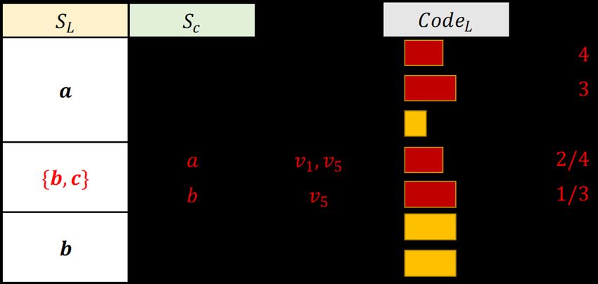
 Fig. 2: Mapping table and inverted database In Fig. 3(a), values are provided in a column under the label
the database is initialized as a basic a-star with one edge fL /fc . The fL means the frequency of the corresponding a-
(core value, leaf value). Hence, all a-stars can be generated star (line) in CTL , while fc is that of the corresponding Sc
by merging two or more lines together. Third, the inverted in the inverted database. Note that, the column fL /fc is not
database allows storing a-stars in a non-redundant way where a part of CTL . Consider the a-star ({a}, {b}) as an example.
each line of the inverted database represents a distinct a-star. This a-star can be represented by Fig. 3(b).
Thus, it is convenient to encode each a-star by appending
a distinct code for each line, instead of building an extra
translation table.

C. MDL with the Inverted Database.
 
 The CSPM algorithm is inspired by the basic framework
for mining compressing patterns of Krimp [20]. Krimp relies
on a two-column standard code table ST and a code table
CT to calculate the total description length of the compressed
database based on the MDL principle. But the data and
pattern types considered by Krimp are simple as it only finds
itemsets (sets of symbols) in a transaction database (a binary Fig. 3: Two code tables and an a-star S = ({a}, {b}) encoding
table) [20]. In this paper, the goal is to discover a-stars in an The description length L(M, I) of a model and inverted
attributed graph, which is more complex as patterns have two database is then calculated by the following equations as
parts which are core values and leaf values. Equation (1):
 Therefore, the Krimp model is adapted to define a model M
that is suitable for a-star patterns. The proposed model type L(M, I) = L(M ) + L(I|M ). (1)
contains two code tables, named CTc and CTL . The former is L(M ) = L(CTc |I) + L(CTL |I). (2)
a traditional two-column code table used to encode coresets,
while CTL is used to encode leafsets. This latter contains Note that, the calculation of L(M ) seen as Equation (2)
pointers to CTc to facilitate appending the codes of coresets is similar to the equation used by the Krimp algorithm. It is
and leafsets to calculate the description length. CTL has a calculated by adding the cost of all columns together.
similar structure to the inverted database. The difference is that The length L(I|M ) is derived directly from the proposed
the third column of CTL contains leaf values’ codes instead inverted database representation by Equation (3):
of sets of positions. X
 Before explaining how CSPM calculates the DL, it is L(I|M ) = L(Scode ) ∗ S(fL ), (3)
 S∈Inew
important to notice that it is necessary to first build the
standard code table ST based on the frequencies of all L(Scode ) = L(Codec ) + L(CodeL ). (4)
attributes in the attributed graph. The standard code table is the
optimal encoding of all attributes without labels and structure where S(fL ) is the frequency of the a-star (line) S in the
information. It contributes to the cost (description length) of new inverted database Inew , which is described using M . And
coresets and leafsets stored in code tables. In the case where L(Scode ) is the code length of S by summing up the code
patterns have a single core value, the format of the code table lengths of its coreset Codec and leafset CodeL .
CTc is the same as that of the standard code table. The CSPM algorithm is designed to find a-stars that indicate
 For the sake of simplicity, we first discuss how to mine a- strong relationships between core values and leaf values ac-
stars having a single attribute value as core values. Then, the cording to the Minimum Description Length (MDL) principle.
more general case of multiple core values will be explained in That is, CSPM is designed to find a-stars meet the following
subsection IV-F. In the case of single-core value patterns, a- two conditions. First, an interesting a-star is supposed to be
stars are found by simply finding the pattern set of SL adjacent frequent to some extent. And the second condition is that the
values for different core values to form the different a-stars. As leaf values need to have high relevance for some core values
example, Fig. 3(a) shows the CTc and CTL code tables for the while being less relevant to other core values. Relevance is
graph depicted in Fig. 1. In that figure, numbers under the label assessed through the conditional entropy, described next.

 5

D. Conditional Entropy m X
 n
 X lij
 L(I|M ) = −s × H(Y |X) = lij log
 j=1 i=1
 cj
 The code length of an a-star is required to calculate the
 m X
 n m X n
DL of a model. The proposed method differs from traditional =
 X
 lij log cj −
 X
 lij log lij (8)
methods such as Krimp that are based on the Shannon entropy j=1 i=1 j=1 i=1
to obtain optimal lengths. There are two reasons. First, the X m m X
 X n

proposed model considers two entities (based on core and leaf = cj log cj − lij log lij .
values), while Shannon entropy is only suitable for the case j=1 j=1 i=1

of one variable. Second, our goal is to evaluate the relevance E. Candidate Generation
between leaf values and core values instead of merely focusing
 The model is built iteratively. After determining all the
on the frequency.
 coresets, the problem is simplified into selecting the leafsets
 Calculating the code Codec of core values in M is only with minimal conditional entropy. An intuitive way of doing
based on the frequency of attribute values in the mapping this is to select the best set of a-stars among all possible
function between vertices and attribute values, as Equation (5). combinations of leafsets with each coreset. But this is time-
To optimally encode leaf values connected to each coreset consuming for large databases. To generate patterns without
 in each a-star, conditional entropy is used as a key measure. assuming that a set of candidates has been previously mined by
 another algorithm as in Krimp, CSPM uses a greedy approach
 that merges the two leafsets that provide the best gain ∆L,
 L(cv) = − log(P (cv)). (5) i.e, in terms of the difference between the DLs before/after
 merging. The gain of a pair represents how much the merge
 step will reduce the DL. Thus, a larger gain is better.
 In information theory, the conditional entropy H(Y |X) Suppose that p is the pair of leafsets {(SLx , SLy )| SLx ∈
measures the cost of describing a random variable Y supposing CTL , SLy ∈ CTL } that CSPM is going to merge. A merge
that the value of another random variable X is given [33]. operation means that a new leafset pattern {SLx ∪ SLy }
Similarly, in this paper, the set of coresets ScM can be regarded will cover all situations where SLx and SLy appear around
as X and the set of leafsets SLM as Y which can be calculated the same coreset. This co-occurrence information is easily
given that the coreset Sc have been obtained. Based on this obtained using the inverted database by intersecting all sets
fact, the relevance of each coreset to its leafset (a set of of positions of the two merged lines that have the same Sc .
leaf values) can be revealed using the conditional entropy. Two parts influence the DL to generate a new pattern {SLx ∪
According to the principle of conditional entropy, the code SLy }. The first one is the cost increase of the new pattern’s
length of each a-star (each line in CTL ) with leafset SL and leafset in the code table, which can be easily obtained through
coreset Sc is given by Equation (6). Hence, the CodeL for the standard code table ST . The other one is the gain ∆L
each line is only determined by the corresponding fL and fc from merging the pair of leafsets. From Equation (8), L(I|M ),
values. Equation (9) is obtained for a simplified calculation of ∆L:
 m m
 0 0
 p(SL , Sc ) fL ∆L = (
 X
 cj log cj −
 X
 cj log cj ) −
 L(Y = SL |X = Sc ) = − log = − log . (6)
 p(Sc ) fc i=1 i=1
 | {z }
 P1
 Then, H(Y |X) is calculated by Equation (7), which rep- m X
 n m X
 n
 0 (9)
resents the average encoding cost of each line in CTL after (
 X
 lij log lij −
 X 0 0
 lij log lij )
using the conditional entropy encoding method. j=1 i=1 j=1 i=1
 | {z }
 P2
 X p(Sc , SL ) where variables with prime as superscript indicate the prop-
 H(Y |X) = − p(Sc , SL ) log 0
 Sc ∈X,SL ∈Y
 p(Sc ) erties of the new code table CTL after the merge operation.
 m X n (7) Note that the number of coresets m does not change during
 X lij lij
 =− log the process because the set of coresets ScM is known.
 j=1 i=1
 s cj
 To better explain the above equation, a detailed analysis of
 In that equation, s is the total frequency of a-stars (lines) in its two parts P1 and P2 is given. It can be observed that P1
the inverted database, which is the sum of fL , m is the total is related to coresets while P2 is related to leafsets. In the
number of coresets, n is the total number of a-stars (lines) in following, for the sake of brevity, the lower case variable x
the inverted database, lij is the frequency fL of the ith leafset is used to denote the fL of the leafset SLx , i.e. x = SLx .fL .
and jth coreset, and cj is the frequency fc of the jth coreset. Similarly, the variable y is used to denote SLy .fL .
 Based on the above equation, the total encoding cost of It can be observed that not all frequencies for each line
the
Pn inverted database is obtained by Equation (8). Note that fL and each coreset fc are changed by a merge operation.
 i=1 lij is equal to the frequency of cj . Suppose C is the coresets that SLx and SLy are both connected

 6

with. For each coreset e ∈ C, fe is the frequency of coreset observed in Fig. 4 that leafsets {b} and {c} are both connected
e, and xye is the co-occurrence frequency of SLx and SLy . to the same coreset {a} of vertices {v1 , v5 } and that they are
By the convenience of the inverted database structure, xye is connected to coreset {b} of vertex {v5 }. Interestingly, the code
obtained by intersecting the positions of a-stars (e, SLx ) and length of leafset {b, c} in CTL corresponding to core value
(e, SLy ) directly. Especially, if xye is equal to zero, the two {a} is much shorter than those of previous ({a}, {b}) and
lines can’t be merged and the gain is equal to zero. Thus, P1 ({a}, {c}). Overall, the database is compressed and its DL is
in Equation (9) can be derived as in Equation (10): reduced by the merge operation.
 X
 P1 = (fe log fe − (fe − xye ) log(fe − xye )). (10) 
 e∈C
 0
 Due to the fact that not all values of lij will become different
from lij after merging, the P2 part is calculated by only sum-
ming up all relative merged lines using Equation (11), where,
Pe means the gain for generating a new a-star (e, SLx ∪ SLy )
by merging lines with core value e.
 X
 P2 = Pe . (11) Fig. 4: Inverted database and CodeL after merging SL pairs
 e∈C ({b}, {c})
 There are three cases to be considered according to the
relationship between xye , xe and ye . F. The Detailed Algorithm
 (1) Partly merged. In this case, the leafsets share some The proposed CSPM algorithm takes as input an attributed
positions but each leafset has some unique positions, graph G (topology and mapping function) and outputs a set
 i.e., xye 6= xe , xye 6= ye . The formulation Pe can be derived of compressing a-star patterns. Algorithm 1 shows the detailed
as Equation (12). procedure. It is divided into two sub-procedures for (1) deter-
 mining and encoding all coresets ScM , (2) and constructing the
 Pe = (xe log xe + ye log ye ) − [(xe − xye ) log(xe − xye )
 (12) final a-stars by finding an approximation of the best leafsets
 +(ye − xye ) log(ye − xye ) + xye log xye ].
 for each coreset using a greedy search. The main steps of
 (2) Two lines totally merged. In this case, xye = xe and CSPM are:
xye = ye . The two lines (a-stars) are merged as a new pattern Step 1: Encode attribute values and core values.
({e}, {SLx ∪ SLy }) because they always appear at the same CSPM reads the mapping function without topology infor-
positions. After merging, there is no a-star ({e}, {SLx }) or mation, where each attribute value appearing at each vertex
({e}, {SLy }) in the inverted database or code table anymore. is seen as an item (symbol). If the user wishes to mine a-
Thus, Pe can be calculated as Equation (13). stars with coresets containing more than one core values,
 a traditional compressing pattern mining algorithm can be
 P2e = (xe log xe + ye log ye ) − (xye log xye ) = xye log xye . applied on a transaction database composed of the attribute
 (13) values of vertices. Several algorithms can be used such as
 (3) One line totally merged. Only one a-star will be
 Krimp [20] and SLIM [25]. In the other case, attribute values
removed by merging. In this case, xye = xe , xye 6= ye or
 are optimally encoded according to their global frequencies.
xye 6= xe , xye = ye , as shown as Equation (14) and (15),
 The result is a standard code table ST of attribute values and
respectively.
 a code table CTc for coresets ScM . Note that CTc is exactly
 Pe = (xe log xe + ye log ye ) − (ye log ye + xye log xye ) the standard code table ST if all coresets have one core value.
 ye (14) Step 2: Construct the inverted database. The inverted
 = ye log + xye log(ye − xye ).
 ye − xye database I is created, which contains leaf values SL , core
 Pe = (xe log xe + ye log ye ) − (ye log ye + xye log xye ) values Sc , and the topology information between core values
 xe (15)
 xe log + xye log(xe − xye ). and leaf values. Besides, each line in the initial inverted
 xe − xye
 database stores the positions of each a-star with only one leaf
 Take Fig. 2 as example. Suppose that the leafsets {b} and value. The inverted database makes it easy to generate merge
{c} of column SL are merged. There are two coresets C = candidates and to cover the database with new patterns.
{{a}, {b}} that these leafsets are both connected with. For Step 3: Generate leafsets merge candidates. Merging
coreset {a}, the P osition of a-stars ({a}, {b}) and ({a}, {c}) candidates allows showing the quality of leafset pairs that
are the same as {v1 , v5 }, which means the two lines can be can be merged as a new pattern. To do so, it is necessary
totally merged as a new pattern (Case 2). And for {b} ∈ C, to calculate the gains ∆L of all possible pairs of leafsets in
the common position is {v5 }. Hence, a-star ({b}, {c}) will be the inverted database. Then, pairs with ∆L > 0 are sorted in
totally merged while the line ({v4 , v5 }−{v5 } = {v4 }) remains descending order to form the final candidates.
for a-star ({b}, {b}) (Case 3). The new inverted database and Step 4: Select a-stars and update the database. A-
code length CodeL after merging are shown in Fig. 4. It is stars are created by merging pairs in candidates that give the

 7

maximal gain. Then, the code table CTL and inverted database n is the leafset count in the inverted database. A leafset is
are updated. Then, Steps 3 and 4 are repeated until there is called related to a merged pair if it contributes a positive gain
no candidate leafset pair that can compress the database more. when merged with a leafset in the merged pair p. For this
A-stars left in model M are the set of patterns we want, where optimization, a dictionary rdict is built to store all related
an a-star with shorter code length will have a higher ranking. leafsets for each leafset of the inverted database.
 Algorithm 3 shows the CSPM-Partial procedure. Line 6
 Algorithm 1: The CSPM algorithm creates the rdict dictionary, which stores key, value pairs.
 input : An attributed graph G with two parts: the adjacency Each key is a leafset and the value is the related leafsets that
 list and the mapping function can be merged with it in candidates. Compared with CSPM-
 output: Compressing a-star patterns Basic, the generate candidates function (line 9 in Algorithm 1)
1 Encode all coresets ScM ; // Step 1 is substituted by an update operation (line 10 in Algorithm 3).
2 CTc ← (Sc , Codec );
3 CTL ← (SL , Sc , CodeL );
 That way, after doing the merge operation in each iteration,
4 I ← (SL , Sc , P osition); // Step 2 only some gains are calculated and updated based on the
5 candidates ←
 previous candidates, instead of enumerating all possible
 M
 generate candidates(SL );// Algorithm 2 pairs and re-calculating their gains again to generate a new
6 repeat candidates.
 7 // select pair with the max. gain ∆L
 8 p ← candidates.pop(); Algorithm 3: The CSPM-Partial algorithm
 9 I, CTL ← merge(p); // Step 4(update I and
 input : An attributed graph G with two parts: the adjacency
 CTL )
 M list and the mapping function
10 candidates ← generate candidates(SL ); // Step 3 output: Compressing a-star patterns
11 until candidates = ∅;
12 return all a-stars in M 1 Encode all coresets ScM ;
 2 CTc ← (Sc , Codec );
 3 CTL ← (SL , Sc , CodeL );
 4 I ← (SL , Sc , P osition);
 Algorithm 2: Generate leafsets merge candidates
 5 candidates ←
 M M
 input : All leafsets SL in CTL , inverted database I generate candidates(SL );// Algorithm 2
 output: A candidate list of leafset pairs 6 rdict ← related dict(candidates)
1 candidates = []; 7 repeat
2 P ← enumerate(SL M
 , 2); 8 p ← candidates.pop();
3 for p ∈ P do 9 I, CTL ← merge(p);
 4 gain ← calculate gain(p, I); // Equation (9) 10 candidates, rdict ← update(p, I); // Algorithm 4
 5 if gain > 0 then candidates.append(p); 11 until candidates = ∅ or len(rdict) = 0;
6 end 12 return all a-stars in M
7 Sort candidates by descending order of gain;
8 return candidates
 Details about the update operation on rdict and candidates
 (after the pair p is merged) are shown in Algorithm 4. ltotal
 and lpart in line 1 contain the totally merged and partly
 V. O PTIMIZATION
 merged leafsets of p, respectively. The overall update proce-
 CSPM can mine a-star patterns efficiently. However, we dure consists of three operations (Remove, Add and Update).
found in empirical experiments that attributes are many while First, totally merged leafsets and related pairs are removed
relationships between attribute values are sparse. Hence, few from rdict and candidates (line 4). Next, all possible related
pairs can improve compression, among a huge number of leafests (rel) are obtained by intersecting rdict[idx] and
possibilities. Besides, few gains are affected by a merge rdict[idy] (line 6) based on the aforementioned observation.
operation and need to be re-calculated and updated. Thus, Each of them (rel) could be merged with the new leafset
it would be time-consuming to calculate all gains of all newa . After calculating the gains, pairs with positive gains are
possible leafset pairs during each iteration. To improve the added to candidates and the related information is recorded in
performance of the candidate generation process, an optimized rdict (line 10-12). Finally, the pairs whose gains are influenced
CSPM version named CSPM-Partial is put forth. It updates by the merge operation are updated in candidates (line 17-
only some of the gains and leafset pairs in candidates after 21). It is a fact that frequencies of a-stars having partly merged
each merge operation on account of the observation that two leafsets are always reduced by the merge operation. Thus, the
leafsets without a common coreset influenced pairs may not contribute to compression anymore,
 will never be merged even if they are merged as a new i,e. the gains are no longer larger than zero. For this reason,
pattern later. More precisely, leafset pairs that are not adjacent the corresponding pairs and their related leafsets are removed
to the same coreset will never have positive gains. Thus, only from candidates and rdict, respectively.
the gains of pairs with related leafsets should be updated after We here analyze the complexity of CSPM-Basic and the
each merge, instead of calculating the gain Cn2 times, where optimized CSPM-Partial. Given an attributed graph G with |E|

 8

Algorithm 4: Update operation VI. E XPERIMENTS
 input : The merged pair p, the inverted database I To evaluate the performance of the proposed CSPM al-
 output: Updated candidates and rdict gorithm Subsection VI-A first presents a runtime and gain
1 ltotal , lpart ← merge state(p); update ratio analysis of the basic CSPM (SPM-Basic), and
2 idx, idy, newa ← p[0], p[1], {p[0] ∪ p[1]}; the optimized version (CSPM-Partial). Then, Subsection VI-B
3 // (1) Remove totally merged leafsets describes some simple a-stars found in real data to intuitively
4 if ltotal 6= ∅ then delete ltotal in candidates, rdict; show that they are meaningful. The quality and usefulness of
5 // (2) Add pairs with new leafset the a-stars as a whole are then evaluated in two application
6 for rel ∈ rdict[idx] ∩ rdict[idy] do scenarios (Subsection VI-C and VI-D).
 7 pair ← (rel, newa );
 8 gain ← calculate gain(pair, I) // Equation (9) First, CSPM is quantitatively assessed for the popular graph
 9 if gain > 0 then attribute completion task. Then, CSPM is used for an industrial
10 rdict[newa ].add(rel); application to extract alarm correlation rules for fault manage-
11 rdict[rel].add(newa ); ment in telecommunication networks. Note that, CSPM-Partial
12 candidates.add(pair); is adopted for the two applications owing to its efficiency.
13 end
14 end A. Evaluation of the CSPM-Partial Optimization
15 // (3) Update influenced pairs
 The first experiments were done to evaluate the benefits of
16 if lpart 6= ∅ then
17 for rel ∈ rdict[lpart ] do using the proposed partial updating optimization.
18 pair ← (rel, lpart ); Algorithms. Three algorithms were compared. The baseline
19 gain ← calculate gain(pair, I) // Equation (9) algorithm is CSPM-Basic without optimization. The second
20 if gain > 0 then update pair.gain in candidates algorithm is CSPM-Partial (CSPM with the partial updating
 else delete pair in candidates, rdict;
 optimization). Moreover, to provide a point of reference for
21 end
22 end experiments, the SLIM algorithm [25] is also adopted for
23 return candidates, mdict comparison. In fact, although SLIM finds simple patterns (sets
 of values that co-occur) without considering inner relationship,
edges, |V | vertices, |A| distinct attribute values. We denote |Ā| it is close to this study as SLIM also is a compression-based
the average number of values per attribute, |SLM | the number of algorithm and it can be easily applied to an attributed graph
leafsets after merging, and |F | the number of generated a-stars. by treating coresets in each adjacency list tuple as items.
The time and space complexity of the two CSPM versions are To our best knowledge, a-star patterns have not been con-
analyzed in as below. sidered before. Note that, graph pattern mining algorithms
 Time Complexity. First, CSPM encodes all coresets. It and summarization techniques mentioned in Section II such
takes O(1) time to insert elements in CTc . Next, all the as VOG and GraphMDL, focus on mining different patterns
attributes are scanned in all vertices to construct the inverted with complicated structure (shown in Table I), which is quite
database, which takes at most O(|E| × |Ā|2 ). Then, patterns different from our work and leads them to have a lower effi-
are generated by doing merges, using at most (|SLM | − |A|) ciency. Hence, these techniques are not included as baselines
iterations. For each iteration, CSPM-basic generates candidates in this work.
(Algorithm 2) in at most O(|SLM |2 ) steps (the last iteration). Datasets. Four benchmark datasets having various charac-
The merge operation is O(1) (add/remove line). CSPM-Partial teristics were used. The statistics are summarized in Table. II,
optimizes this procedure by only considering some candidate where |ScM | gives the number of coresets in the inverted
pairs, database. DBLP [34] is a citation network indicating co-author
 relationships (edges) between researchers (vertices) during
 and the worst case is O(|SLM |) in each iteration. But years 2006-2010. Attribute values are the conferences/journals
generally, few attributes are highly correlated with the merged a person has published in. The DBLP-Trend [35] is a variant of
leaves. Thus, the time complexity of recalculating gains in DBLP where the attribute indicates trends about publications.
each iteration is O(k), k  |SLM |. This is why CSPM-Partial For example, (ICDE+, ICDE-, ICDE=) indicates that the
outperforms CSPM-Basic in experiments. number of publications in ICDE has increased, decreased,
 Space Complexity. The dataset is stored as an inverted and stayed the same since the previous year, respectively.
database, which is updated to generate a-stars. Thus, CSPM- The USFlight [36] dataset contains data about flights (edges)
Basic uses O(|F |) space. The space complexity of CSPM- between US airports (vertices) in 2005. The Pokec dataset1
Partial is O(|F | + |R|), where |R| is the additional memory indicates friendship relationships (edges) between persons
for keeping potentially related leaf-values, with the worst case (vertices) on the Pokec social network. The attribute values
of O(|A| × |A − 1|). store the musical tastes of users.
 (1) Runtime. In the first experiment, the influence of the
 But for real applications, it is unlikely that all attributes are proposed optimization on the runtime was evaluated by com-
correlated with each other due to sparsity. Thus, the additional
memory usage is generally very small. 1 https://stanford.io/3oZH9EI

 9

TABLE II: Statistics about datasets of the two algorithms for each dataset from the first to the
 Dataset DBLP DBLP-Trend USFlight Pokec last iteration. Recall that, during an iteration and after merging
 #Nodes 2,723 2,723 280 1,632,803 two leafsets, merge candidates are updated. Moreover, the gain
 #Total edges 3,464 3,464 4,030 30,622,564 update ratio represents the ratio of gain values that are added
 |ScM | 127 271 70 914
 Category Citation Citation Airport Music or updated out of the total number of possible calculations in
 each iteration.
paring CSPM-Partial with CSPM-Basic. Results are shown in It can be observed that, CSPM-Partial often obtains a better
TABLE III. Note that, the result of CSPM-Basic on the Pokec gain update ratio compared with CSPM-Basic. This is why
dataset is written as (−) because CSPM-Basic was not able to CSPM-Partial performs well on the used datasets such as
terminate after 48 hours. Three observations are made. DBLP and Pokec.
 TABLE III: Runtime comparison B. Pattern Analysis
 Runtime (s) To evaluate the interestingness of patterns discovered by
 Dataset SLIM CSPM-Basic CSPM-Partial
 the proposed CSPM algorithm, a manual inspection of the
 DBLP 4.69 43.13 0.98 discovered patterns was performed. Besides, patterns with
 DBLP-Trend 48.69 956.61 25.46
 USFlight 1.25 10.16 1.43 small code lengths are more frequent and have the strongest
 Pokec 166,678.3 – 1,403.21 relationship between their core and leaf values.
 (1) DBLP. Two patterns mined in DBLP and DBLP-Trend
 First, the CSPM-Basic algorithm is approximately 10 times are depicted in Fig. 6(a). It was found that, there are many
slower than SLIM. This result is reasonable since CSPM-Basic pattern occurrences where a researcher published a paper in
solves a problem that has two variables (core and leaf values) ICDM and EDBT during a year, and his/her co-authors
and it considers the graph topology which is more complex. published in P ODS, ICDM and EDBT during the same
Moreover, CSPM-Basic merges and updates candidate pairs year. This is reasonable as P ODS, ICDM , and EDBT
without using any optimization. belong to the same research area (data-mining), and generally,
 co-authors of a paper are interested in the same research areas.
 (a) DBLP (b) DBLP-Trend The pattern of Fig. 6(b) from DBLP-Trend can be interpreted
 in a similar way. But a difference is that patterns found in
Update ratio(%)

 Update ratio(%)

 DBLP-Trend contain information about trends.

 −
 
 i-th iteration i-th iteration 
 (c) USFlight (d) Pokec
 + DMK − KDD= 
 Update ratio(%)
 Update ratio(%)

 = −

 (a) DBLP (b) DBLP-Trend (c) Pokec
 Fig. 6: Example a-stars from DBLP, DBLP-Trend and Pokec
 i-th iteration i-th iteration
 Fig. 5: Comparison of gain update ratio (2) USFlight. An example pattern from the USFlight dataset
 is: ({N bDepart−}, {N bDepart+, DelayArriv−}), which
 Second, it was found that, the optimized algorithm, CSPM- means that, if the number of departure flights is reduced in
Partial, is considerably faster than the CSPM-Basic. Especially an airport, there is a high chance that some connected airports
for Pokec which is a large dataset. This result demonstrates will have an increase in their number of departure flights and
that the proposed optimizations can make the algorithm more a decrease in their number of delayed flights.
efficient. (3) Pokec. Pokec dataset contains the music preferences of
 A third observation is that, the runtime of CSPM-Partial people from different communities. Some interesting patterns
increases as the number of coresets increases. In fact, CSPM- were also discovered in this dataset using CSPM such as:
Partial optimizes the performance by generating several new ({rap}, {rock, metal, pop, sladaky}). This pattern has a
leaf values during each iteration. However, the more leaf short encoding length and a high frequency which means that it
values that CTL contains, the more the frequency of gain greatly contributes to the reduction of the conditional entropy.
pairs calculations for each iteration. Therefore, the runtime This pattern seems reasonable because some music types such
is increased. as rock, metal, pop, sladaky, and rap are preferred by young
 Overall, the optimized algorithm CSPM-Partial achieves people. Another pattern is found and it shows the music
high performance in terms of runtime especially for large preferences of older people: ({disko}, {oldies, disko}).
datasets.
 (2) Gain update ratio. The second experiment is performed C. Node Attribute Completion
to compare the relative amount of gain calculations achieved In this section, we quantitatively assess the patterns to
by the two CSPM versions. Fig. 5 shows the gain update ratio check whether CSPM can reveal underlying characteristics of

 10

the data. More precisely, we apply CSPM to a graph-related Attribute-missing Training Probabilities
 Neural
classification task, namely node attribute completion [8]. graph
 network
Attribute-missing graph completion is useful for numerous ？
 ⊗
real-world applications. Thus, various algorithms have been
proposed [8], [37], [38], [39] to deal with ths task. Intuitively, Scores
 CSPM
if attribute-stars extracted by CSPM can summarize well ？ model
the data characteristics, incorporating mined patterns into the Fig. 7: The whole process of the attribute completion task
existing algorithms should improve or at least not degrade their using CSPM
performance.
 We first present a scoring scheme which enables CSPM for Experiments are conducted on three benchmark citation
the node completion task. It is based on the idea that a missing networks in which attributes are categorical, namely Cora
attribute value can be treated as a coreset with a core value [40], Citeseer [41], and DBLP [34]. Similarly to [8], the
and those of the neighbor nodes as leaf-values in an a-star. performance is evaluated according to the Recall@K and
Then, a core value in an a-star with a smaller code length NDCG@K [42], where larger values indicate better results.
is more likely to be an attribute value of the targeted node. Specifically, the Recall reflects the correctness of the predicted
Therefore, we can score all possible attribute values using the attributes and the NDCG assesses ranking quality.
code tables produced by CSPM. Note that DBLP is evaluated with a smaller K as it has
 The scoring module is summarized in Algorithm 5. In brief, less attribute values per node. The results are summarized in
given the a-star set M of CSPM and the attributes of the TABLE IV. It can be seen that, by integrating the a-stars-
neighbors, the algorithm will return the scores of all possible based scoring module into the attribute completion process, all
attribute values for a targeted node v. In general, it is difficult the baseline algorithms are improved with different degrees.
to perfectly match the leaf-values in the leafset of an a-star The most significant improvement is for NeighAggre or VAE
with the attribute values of a neighbor. Thus, a weight is which have relatively poor performance. These observations
introduced to evaluate the similarity between leaf values in the confirm that CSPM can successfully summarize the underlying
leafset of an a-star and that of the neighbors of v. Intuitively, characteristics of the given data.
a leafset that is not similar to a set of neighbors will have
a large weight w. As a result, it has a small score cl which D. Alarm correlation analysis
indicates that the corresponding core-values are less likely to Telecommunication networks are cornerstones of the com-
be an attribute value of v. munication systems in modern society. Ensuring high-quality
 services in complex and large telecom networks is impor-
 Algorithm 5: The scoring module of CSPM tant and challenging since millions of faults and alarms
 input : An attributed graph G with n attribute values, the are triggered across the devices everyday. Thus, discovering
 model M , a node v with missing attribute values relationships between these alarms and filtering trivial alarms
 output: Scores for all possible attribute values from important ones is critical to locate faults.
1 scores ← [−∞]n×1 ; // Set scores to -∞ Recently, several studies have applied pattern mining tech-
2 neighbors ← neighbor attributes(v);
 niques for alarm correlation analysis. Wang et al. [45] de-
3 foreach a-star S in M do
 4 Scode ← code length(S); // Equation (4) signed and deployed an alarm management system called
 5 w ← similarity(SL , neighbors); // SL :leafset of AABD (Automatic Alarm Behavior Discovery) where the
 S alarm correlation module mines frequent patterns in alarm
 6 cl ← −w × Scode ; logs via sequential pattern mining [46], [47]. The discovered
 7 if cl > scores[Sc ] then
 patterns are then used to generate rules indicating that an alarm
 8 scores[Sc ] ← cl; // Sc :coreset of S
 9 end may be caused by another alarm. These rules are used to
10 end perform alarm compression (reduce the number of alarms pre-
11 return scores sented to maintenance workers). For instance, (Low_signal,
 {Link_degrader, Microwave_stripping}) is an
 Based on the fact that CSPM is designed to learn the alarm rule, suggesting that the cause alarm Low_signal
underlying correlations between attribute values, it is suitable may be triggering derivative alarms (i.e., Link_degrader
to assist other attribute completion models. This is done by and Microwave_stripping). The alarm compression is
integrating CSPM with attribute scoring into existing node achieved by only showing Low_signal to the maintenance
attribute completion models. The prediction process is illus- workers when they appear simultaneously.
trated in Fig. 7. Besides, the output of a graph completion As AABD utilizes pattern mining algorithms which are
model for each vertex is a vector containing values indicating not parameter-free, the quality of results is sensitive to the
the possibilities that the attribute values appear while the parameter values. Moreover, AABD ignores the connections
vector obtained by the CSPM model records the scores of between network devices and the alarm importance in a mined
each attribute. In the proposed approach, the two vectors are rule (i.e., cause alarm or not) have to be inferred by the
normalized separately and then multiplied to get final scores. experts knowledge. To solve the above problems, the ACOR

 11