Development of a local empirical model of ionospheric total electron content (TEC) and its application for studying solar ionospheric effects - Nature

Page created by Stacy Welch
 
CONTINUE READING
Development of a local empirical model of ionospheric total electron content (TEC) and its application for studying solar ionospheric effects - Nature
www.nature.com/scientificreports

                OPEN              Development of a local empirical
                                  model of ionospheric total electron
                                  content (TEC) and its application
                                  for studying solar‑ionospheric
                                  effects
                                  Pantea Davoudifar1,2*, Keihanak Rowshan Tabari1, Amir Abbas Eslami Shafigh1,
                                  Ali Ajabshirizadeh3, Zahra Bagheri4, Fakhredin Akbarian Tork Abad2 & Milad Shayan1

                                  Regular and irregular variations in total electron content(TEC) are one of the most significant
                                  observables in ionosphericstudies. During the solar cycle 24, the variability of ionosphere isstudied
                                  using global positioning system derived TEC at amid-latitude station, Tehran (35.70N, 51.33E).
                                  Based on solar radioflux and seasonal and local time-dependent features of TEC values, asemi-
                                  empirical model is developed to represent its monthly/hourlymean values. Observed values of
                                  TEC and the results of oursemi-empirical model then are compared with estimated values of
                                  astandard plasmasphere–ionosphere model. The outcome of this modelis an expected mean TEC
                                  value considering the monthly/hourly regulareffects of solar origin. Thus, it is possible to use it
                                  formonitoring irregular effects induced by solar events. As a result,the connection of TEC variations
                                  with solar activities are studiedfor the case of coronal mass ejections accompanying extremesolar
                                  flares. TEC response to solar flares of class X is wellreproduced by this model. Our resulting values
                                  show that the mostpowerful flares (i.e. class X) induce a variation of more than 20percent in daily TEC
                                  extent.

                                   In the Earth’s ionosphere, the variability of space weather is easily reflected in TEC. As the total number of
                                   electrons is measured along a vertical column of one square meter cross-section (1 TEC Unit (TECU)
                                  = 1 × 10¹⁶ electrons m−2) from the height of a GPS satellite (∼ 20, 000 km) to the receiver, thus TEC char-
                                   acterizes variations in both ionosphere and p    ­ lasmasphere1.
                                       Until now, various techniques have been used to empirically measure TEC. Some examples include:
                                  ­ionosondes2,3, incoherent backscatter r­ adars2,4,5, Faraday Rotation (FR) in beacon satellite s­ ignals2,6–8, altimeter
                                   satellite systems, and Global Navigation Satellite Systems (GNSS)1,9. The Global Positioning System (GPS) satel-
                                   lites, provide an effective and low-cost method to measure TEC ­values10,11 as a function of time for a specific
                                   location on the Earth. GPS signal, propagating through the ionosphere, is advanced in phase and delayed in
                                   time. As a result, values of carrier phase and pseudo-range combined L-band frequencies (L1 carrier:1575.42
                                   MHz and L2 carrier: 12227.60 MHz) are used to evaluate T          ­ EC12–15.
                                       TEC values are subject to both temporal/spatial and regular/irregular v­ ariations16,17. Spatial variations describe
                                   those related to the location on the Earth (i.e. equatorial anomalies etc), whilst temporal variations are related to
                                   time (i.e. universal or local). Where, regular variations include periodic changes in TEC values, irregular ones
                                   show the temporal effects of phenomena such as solar events and geomagnetic storms.
                                       Investigating TEC variations reveals the main physical processes which are responsible for the ionospheric
                                   behaviour. Generally speaking, the changes in TEC values are mainly connected with: the condition of the Earth’s
                                   magnetic field, the Earth’s rotation (which induces diurnal effects), the Earth’s position around the Sun (which
                                   induces observed seasonal effects) and the solar activity levels. Whilst diurnal and seasonal effects are considered
                                   as regular effects, the solar activity levels and its effect on the Earth’s magnetic field may produce both regular and

                                  1
                                   Research Institute for Astronomy and Astrophysics of Maragha (RIAAM), University of Maragheh, Maragheh,
                                  Iran. 2Iranian Space Agency (ISA), Tehran, Iran. 3Physics Department, University of Tabriz, Tabriz, Iran. 4Institute
                                  for Research in Fundamental Sciences (IPM), School of Particles and Accelerators, Tehran, Iran. *email:
                                  p.davoudifar@maragheh.ac.ir

Scientific Reports |   (2021) 11:15070                 | https://doi.org/10.1038/s41598-021-93496-y                                                      1

                                                                                                                                                    Vol.:(0123456789)
www.nature.com/scientificreports/

                                            irregular variations. Irregular variations in TEC are mainly due to Traveling Ionospheric Disturbances (TID)18–20
                                            and/or ionospheric or geomagnetic ­storms21.

                                            Solar variability and the ionosphere
                                             Geomagnetic storms are the results of variations in the solar currents, plasmas and the Earth’s magnetosphere
                                             which is dominated by the magnetic field. These variations are simply induced to the Earth’s surrounding by
                                             solar wind or by plasma pockets from the Sun, travelling in the solar system with their frozen in magnetic fields
                                             (i.e. CMEs or totally “Ejecta”s)22–25. In fact, the most extreme geomagnetic storms are associated with Coronal
                                             Mass Ejection (CME) ­events26 in most cases accompanying the solar flares.
                                                 Considering their peak fluxes, solar flares are classified as X, M and C classes ( < 10−4 , ∼ 10−5 − 10−4 and
                                            > 10−4 watts per square meter for C, M and X classes respectively). Sudden increased radiation during a solar
                                             flare, causes extra ionization of the neutral components on the day-side of the Earth’s a­ tmosphere27. Whilst soft
                                             X-ray and far UV fluxes enhance ionization in the E-region, hard X-ray component is responsible for enhanced
                                             ionization in the D-region. Electrons with approximate peak energies of a few keV cause ionization in lower E
                                             region and solar proton events with energies more than 100 MeV cause ionization much deeper into the atmos-
                                             phere, namely into the D-region28–30.
                                                 The time interval for Solar flare effects on the ionosphere, maybe divided to three main parts: (A) 0 ∼ 1 hour;
                                             increased photo ionization in the day-side, the flare energetic particles arrive shortly after the flare photons, (B)
                                             1 hour ∼ 4 days; Arrival of energetic particles accelerated in fast interplanetary shocks (ICMEs), and (C) 1 day
                                            ∼ 4+days, the effect of interplanetary electric field on the ionospheric height on day and night-sides31.
                                                 The solar cycle 24, was started with low solar activity. During this “deep minimum”, the relationship between
                                             solar EUV flux and F10.7 index was deviated from its behavior in the past solar m    ­ inimum32. Furthermore, the
                                             International Reference Ionosphere (IRI) model overestimated TEC values for this p      ­ eriod33–36, thus developing
                                             semi-empirical models matters a lot.
                                                 The study of ionospheric response to solar flares, first was introduced by Afraimovich, et al.,37–40. In their
                                             studies, Afraimovich et al. used TEC values directly and analyzed the observed fluctuations considering varia-
                                             tion amplitude and background fluctuations. Other researchers also studied the signature of Solar flares on TEC
                                            ­values41,42 and monitored TEC variation during geomagnetic s­ torms43. These studies are essentially based on
                                             analyzing observed TEC values without trying to remove long term regular effects. In some cases the ionospheric
                                             response to solar flares was studied using more than one s­ tation41. Choi et al.43 showed ionospheric TEC vari-
                                             ation over a region to study the response to storm periods. Instead we offer a method to study the signature of
                                             solar events even for one station. Using a semi-empirical model we produce expected hourly/daily mean values
                                             of TEC for one station during different phases of a solar cycle. Because of the applied method, these mean values
                                             represent the regular behavior of TEC. Thus, it is possible to use the results to observe the effect of irregular
                                             events such as solar flares and coronal mass ejections.

                                            Justification and outline of our semi‑empirical model
                                             Due to the Earth’s magnetic field, three latitudinal regions are recognized in the ionosphere: low-latitude or
                                             equatorial, mid-latitude and high-latitude regions. Usually, the low-latitude region contains the highest values
                                             of TEC whilst the mid-latitude region is considered as the least variable region of the ionosphere and it contains
                                             the most predictable variations of T­ EC9. It is shown that even in deep solar minimum a strong correlation with
                                             the solar indexes still e­ xist13.
                                                 When developing a semi-empirical model, it is essential to remove the disturbed periods of geomagnetic
                                            ­storms44,45. The disturbance degree is directly related to the strength of the disturbing phenomena.
                                                 The strength of a geomagnetic storm is usually measured using geomagnetic indexes. Amongst them Kp, Dst
                                             (disturbance–storm time) (∼ 20 − 30◦ latitudes), SYM-H and ASY-H (∼ 40 − 50◦ latitudes) ­indexes46–48 provide
                                             good information about the storm condition. Generally, after the storm sudden commencement, three phases are
                                             recognized during a ­storm49: The initial (with an increase in Dst by 20 to 50 nT; for tens of minutes); main (with
                                            a Dst decreasing to less than −50 nT; 2–8 hours) and recovery phases (Dst changes from its minimum value to
                                            its quiet time value; 8 hours and above)44.
                                                 SYM and ASY (both -D and -H) indexes are acquired from observations of magnetic fields at low and mid-
                                             latitudes (WDC, Kyoto) and describe the development of a magnetic storm. Compression of the dayside mag-
                                             netosphere in the initial phase of a storm induces positive Dst values (as well as positive SYM-H values) whilst
                                             magnetic reconnection and ring current formation induce strongly negative values during the main ­phase50.
                                             SYM-H index is considered to be an analogues of Dst in many ­studies51–53. On the other hand, it is shown that
                                            for Dst variations greater than 400 nT, these two values may d  ­ iffer54. In more detailed studies, it is recommended
                                             that SYM-H index can be used as a high-resolution Dst i­ ndex55,56, of course with different scales for the defini-
                                             tion of moderate s­ torms56.
                                                 We have considered moderate, intense and super-storms (moderate: − 50 nT > Dstmin > − 100 nT ; intense:
                                             − 100 nT > Dstmin > − 250 nT ; super-storm: Dstmin < − 250 nT; During quiet times: − 20 nT < Dst < + 20 nT)
                                            to be the most probable reason of disturbed time periods and consequently designed a suitable filter to detect
                                            and remove them.

                                            Database
                                            The GPS-TEC d   ­ ata57,58 used in this research were detected by GNSS receiver Tehran (lat: 35.70N, lon: 51.33E)
                                            for a period of 11 years from low to high (2008–2013) and high to low (2014–2018) solar activity. The temporal
                                            resolution of the data is 30 seconds and received online from IONOL​AB (to receive data for a time period, one

          Scientific Reports |   (2021) 11:15070 |               https://doi.org/10.1038/s41598-021-93496-y                                                     2

Vol:.(1234567890)
www.nature.com/scientificreports/

                                                                                       Dst versus DOY
                                               100

                                                50

                                  Dst (nT)
                                                 0

                                                -50

                                               -100

                                               -150
                                                              50          100         150          200       250    300          350
                                                                                            DOY (2017)
                                                                                      SYM-H versus DOY
                                               100

                                                50
                                  SYM-H (nT)

                                                 0

                                                -50

                                               -100
                                                      -43 nT-50 nT

                                               -150
                                                              50          100         150          200       250    300          350
                                                                                            DOY (2017)

                                  Figure 1.  Dst and SYM-H behavior during the year 2017.

                                  can use scripting with IONOLAB-TEC/STEC Software), which provides TEC data with a resolution of 30 seconds
                                  from Receiver Independent Exchange Format (RINEX) files.
                                      Production of ionization is mainly controlled by the solar EUV radiation. Due to unavailability of a suitable
                                  database of solar EUV radiation, solar radio flux (i.e. F10.7) is considered as a substitute index of solar activ-
                                  ity which is reflected in our model. The daily F10.7 data were collected from OMNIW​EB. Other parameters
                                  concerning IMF, solar wind and plasma parameters and activity indexes were acquired from OMNIW​EB:​ High
                                  Resol​ution​ OMNI.
                                      Processing the above data, the hourly/monthly mean values of the solar index (F10.7) and the ionospheric
                                  parameter TEC were prepared which allow us to study the variability of TEC with solar events.
                                      Solar events in the above time interval were selected from Watanabe et al (2012)59 XRT flare​ catal​ogue and
                                  compared with the information from SOHO LASCO​CME catal​ogue. To study the solar radio bursts RADIO
                                  SOLAR TELESCOPE NETWORK 1 Sec Solar Radio Data (SRD) files from RSTN were used.
                                      SYM and ASY (both -D and -H) indexes are acquired from observations of magnetic fields at low and mid-
                                  latitudes (WDC, Kyoto).

                                  SYM‑H versus Dst
                                  It is not easy to find a unique description for the storm’s degree based on SYM-H values, specially for the com-
                                  mon definition of a moderate storm based on Dst values. In a closer look Dst and SYM-H do not behave like
                                  each other as it is previously ­mentioned55. In some cases a moderate storm condition starts with a SYM-H index
                                  lower or higher than its Dst value (it can fluctuate around 20 nT). Thus, first we decided to re-scale SYM-H based
                                  on Dst for solar cycle 24.
                                       A first and a simple choice was to use the same limits calculated for the period of 1985 through ­200956 or
                                  1981 through 2­ 00255. For ­instance56:
                                                                                    sym-h = 0.95 ∗ Dst + 4.5 nT,                                  (1)
                                  gives a SYM-H index of − 43 nT for starting moderate storms (i.e. Dst of ∼ −50 nT). A sample of “storm time
                                  intervals” consisting of the time intervals of 1000 storms (of the moderate and above degrees, picked by their
                                  Dst values) was used as the test sample for solar cycle 24. As our first step, the entire period of 2009–2018 in the
                                  search of a proper lower limit of SYM-H (i.e. for marking moderate storms and above) was studied.
                                      For instance, a comparison between Dst and SYM-H indexes is shown in Fig. 1, where it is seen that in the
                                  case of moderate storms, considering − 43 nT as the lower limit of SYM-H leads to the detection of more storms,
                                  so the starting value is important. Using − 46 nT gives better result for our data set in this period.
                                      Considering the behavior of power spectrums of Dst and SYM-H (Fig. 2), some differences are seen (com-
                                  pared with the period of 1981–200255). Our power spectrums seems more noisy (Fig. 2) and as a result the peaks
                                  are not sharp as previously reported for the time interval of 1981–2002.
                                      Plotting the probability distribution functions of Dst and SYM-H also provides some information about the
                                  behavior of these values over the time interval of 1981–2018 (Figs. 3, 4).

Scientific Reports |   (2021) 11:15070 |                        https://doi.org/10.1038/s41598-021-93496-y                                          3

                                                                                                                                               Vol.:(0123456789)
www.nature.com/scientificreports/

                                            DST and SYM-H Power spectrum (nT2/Hz)
                                                                                                                                                            24 hours

                                                                                    1010

                                                                                    105

                                                                                                             6 months
                                                                                    100                                  1 months
                                                                                           Top curve: SYM-H power spectrum * 1e+6
                                                                                           Bottom curve: Dst

                                                                                      10-9          10-8          10-7         10-6              10-5            10-4        10-3             10-2
                                                                                                                               Frequency(Hz)

                                             Figure 2.  Dst and SYM-H power spectrum during 2009–2018.

                                                                                                                                                                                    Data points
                                                                          0.025
                                                                                                                                                                                    Quiet I
                                                                                                                                                                                    Quiet II
                                                                                                                                                                                    Active
                                                                                    0.02                                                                                            Fitted Curve
                                            Probability Density

                                                                          0.015

                                                                                    0.01

                                                                          0.005

                                                                                      0
                                                                                      -150                 -100              -50                        0               50                     100
                                                                                                                                      Dst (nT)

                                             Figure 3.  Probability Distribution Functions of Dst during 1981–2018.

                                                                                                                                                                                    Data points
                                                                          0.025
                                                                                                                                                                                    Quiet I
                                                                                                                                                                                    Quiet II
                                                                                                                                                                                    Active
                                                                                    0.02                                                                                            Fitted curve
                                            Probability Density

                                                                          0.015

                                                                                    0.01

                                                                          0.005

                                                                                      0
                                                                                      -150                 -100              -50                        0               50                     100
                                                                                                                                    SYM-H (nT)

                                             Figure 4.  Probability Distribution Functions of SYM-H during 1981–2018.

                                                                                    For example it is seen that the sum of 3 gaussian distributions provides a good fit to both Dst and SYM-H

          Scientific Reports |   (2021) 11:15070 |                                                    https://doi.org/10.1038/s41598-021-93496-y                                                     4

Vol:.(1234567890)
www.nature.com/scientificreports/

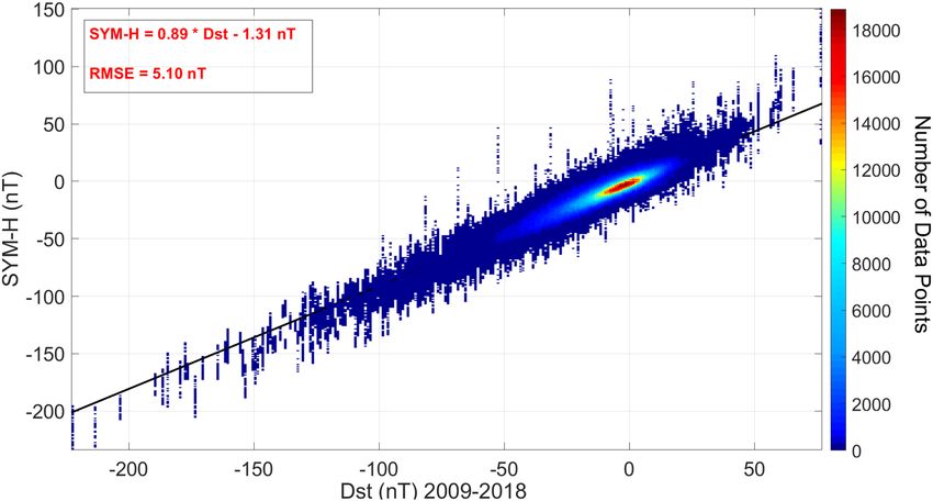
                                  Figure 5.  The Distribution of storm times SYM-H versus Dst during 2009–2018. The best fit line is shown in
                                  black and equation in red.

                                  distributions:
                                                                                  2                            2                            2
                                                                                      /c12                         /c22                         /c32      (2)
                                                             P(x) = A1 · e(x−b1 )            + A2 · e(x−b2 )              + A3 · e(x−b3 )

                                        Both Dst (Fig. 3) and SYM-H (Fig. 4) show 3 populations in their probability distributions, with (integrated)
                                   probability density values of: ∼ 0.43 (µ, − 18.56 nT and σ , 14.98 nT), 0.39 (µ, − 5.10 nT, and σ , 10.18 nT), 0.18
                                    (µ, − 36.72 nT, and σ , 31.32 nT) and 0.45 (µ, − 4.42 nT, and σ , 9.77 nT) , 0.39(µ, − 17.96 nT, and σ , 15.63 nT),
                                    0.16 (µ, − 33.45 nT, and σ , 31.49 nT) respectively. In comparison the gaussian distribution with higher popula-
                                    tion (− 18.56 nT) occurs at higher SYM-H values (− 4.42 nT) and the lowest population (around ∼ − 30 nT) has
                                    a difference of 3 nT in the peak position for Dst and Sym-H whilst showing higher values of σ (i.e. 31.32 and
                                   31.49 nT) compared with two other distributions. In comparison, only less than ∼ − 10 percent of the events
                                    were recorded in the domain of − 50 nT and lower.
                                        Compared with the method used by Wansliss and S­ howalter55, we see three spectrums. One Active and two
                                    Quiets (QI and QII). QI and QII cross the Active spectra at − 46nT and − 28nT respectively.
                                        Through correlation studies for the time period of 1960–2001, the behavior of geomagnetic indices are shown
                                    to be correlated the best with Interplanetary Magnetic Fields (IMF)60 embedded within the solar wind. Solar
                                   magnetic field originates in convention layer and extends into the corona and the solar wind. Fast solar wind
                                   originates from coronal holes whilst slow solar wind originates at the edge of coronal ­holes61. Solar wind carries
                                    the strongest fields at solar maximum which are due to interplanetary coronal mass ejections and at this period
                                    the Earth experiences a broad range of solar wind ­velocities62,63. Around solar minimum, the coronal holes are
                                    located at the poles. When the magnetic quadrupole moment dominates over the dipole moment, a number of
                                    coronal holes appear at mid-latitudes, this is a typical behaviour in a solar cycle during solar maximum. At solar
                                    cycle 24 a deeper decrease of dipole component occurred in solar ­minimum63. During the deep solar minimum
                                    between cycles 23 and 24, the evolution of coronal holes and its connection to solar wind speed is discussed in
                                  ­details64 and a secondary peak in solar wind speed distribution is seen for 2007–2008. During solar cycle 24,
                                   solar wind speed is shown to have the highest correlation with geomagnetic indices, Ap and Dst, with zero time
                                   ­delays65. Jackson et al.66, used Current Sheet-Source Surface (CSSS) ­model67 to determine Geocentric Solar Mag-
                                    netospheric (GSM) Bz field. They found that the daily variations of Bz are also correlated with geomagnetic Kp
                                    and Dst index variations over 11-year period of National Solar Observatory Global Oscillation Network Group
                                    (data. GONG). Thus it seems that the existence of 2 quiet spectrum in Figs. 3 and 4 is not accidental and may
                                    reflect the different situation of the solar cycle 24.
                                        More numerical studies help to decide about the filters for executing disturbed time intervals. A linear fit to
                                    the scatter plot of SYM-H versus Dst (Fig. 5) gives the linear relationship:
                                                                           sym-h = 0.89 ∗ Dst − 1.31 nT,                                                  (3)
                                  Inserting the limit of − 50 nT for Dst gives the limit of SYM-H ∼ − 45.81 nT, comparable with the method applied
                                  by Katus et. al.56 (i.e. formula 1).

Scientific Reports |   (2021) 11:15070 |               https://doi.org/10.1038/s41598-021-93496-y                                                           5

                                                                                                                                                       Vol.:(0123456789)
www.nature.com/scientificreports/

                                                                                      ASY-H versus DOY
                                                    100

                                            ASY-H
                                                     50

                                                      0
                                                      110    110.5   111     111.5     112     112.5      113     113.5     114     114.5      115
                                                                                            DOY
                                                                                      SYM-H versus DOY
                                                     50
                                             SYM-H

                                                      0

                                                     -50
                                                       110   110.5   111     111.5     112     112.5      113     113.5     114     114.5      115
                                                                                                DOY

                                            Figure 6.  ASY-H and SYM-H behavior during geomagnetic storm of 22 April 2017 (DOY 112). The filter
                                            discussed in the section "Applied Filter" were applied to mark disturbed time intervals. Solid lines (black, green
                                            and red) show the first occurrence of SYM-H value bellow − 46 nt. Dashed lines (black, green, red) show the
                                            start of related sub-storms considering the variation of ASY-H.

                                            Applied filter
                                            Instead of considering Dst v­ ariations68, our storm finding procedure is based on the variation of SYM-H (for-
                                            mula 3) whilst ASY-H is used to find the storm onset times.
                                               Different steps of our filtering algorithm are listed as below:

                                            • Generally, SYM-H values below − 46 nT were considered as the start of a possible storm.
                                            • A second filter is considered to detect storm onset times more precisely using ASY-H and SYM-H values.
                                              Observing a sharp positive peak in ASY-H values shows the sub-storm o    ­ nsets69 prior to / or after occurrence
                                                                                 70,71
                                              of a moderate geomagnetic s­ torm . So in this method the onset times of the storms were highlighted
                                              observing the behavior of ASY and SYM (especially H) indexes.
                                            • For the storm time periods if there is only one record with the value of “at or below” − 46 nT in the selected
                                              period, the time period was not removed.
                                            • The recovery time also is considered (forwarded in time from the selected starting point) using ASY-H, up
                                              to the deepest local minimum after the starting point (if it does not result in less than 2 hours).
                                            • The specified time periods were recorded and then excluded from raw data of TEC before calculating the
                                              desired mean values.

                                            We examined our procedure for a test sample of storm time intervals during 1/1/2017–1/1/2018. The coincidence
                                            was 91.2 % using only steps 1 and 2, 97 % when adding step 3.
                                                The above method is applied upon the whole time interval of cycle 24, backward in time. It is obvious that
                                            in comparison with the method applied by Badeke et al.68, we remove less time periods (they have removed 36
                                            hours for each considered storm).
                                                As an example of how this procedure works, the time interval of a geomagnetic storm (22 April 2017) (SGAS
                                            Number 112 Issued at 0254z on 22 Apr 2017) is shown in Fig. 6.
                                                To study this storm a time period of 5 days is drawn (2 days before and 2 days after the reported date). The
                                            data was acquired from WDC, Kyoto.
                                                Applying this method, in the first step 58 points were recognized with a SYM-H value below − 46 nT.
                                                The first recognized occurrence of a SYM-H value below − 46 nT is on DOY 113, 23 April 2017, 00:08:00.
                                            Prior to this time, considering the variation of ASY-H, the start of a sub-storm is recognized on 22 April 2017,

          Scientific Reports |   (2021) 11:15070 |               https://doi.org/10.1038/s41598-021-93496-y                                                  6

Vol:.(1234567890)
www.nature.com/scientificreports/

                                                                                 Ionospheric Hysteresis Effect
                                        25                                                      20
                                               2009-2013                                                2009-2013
                                        20     2014-2018                                                2014-2018
                                                                                                15

                                 TECU
                                        15
                                                                                                10
                                        10
                                                                              April, LT 01:00                                     April, LT 06:00
                                         5                                                     5
                                          60       80        100       120        140       160 60          80      100     120        140       160
                                        60                                                    25
                                               2009-2013                                                2009-2013
                                        50     2014-2018                                        20      2014-2018
                                 TECU

                                        40
                                                                                                15
                                        30
                                                                                                10
                                        20                                   April, LT 12:00                                       April, LT 24:00
                                                                                                5
                                         60        80        100       120       140        160 60           80     100     120        140       160
                                                                                             F10.7

                                  Figure 7.  Ionospheric Hysteresis Effect for the time period of 2009–2018.

                                  21:33:00. Thus, the onset time for this storm was 22 April 2017, 21:33:00 and the time period from 4/22/2017
                                  21:33:00 to 4/23/2017 00:08:00 was excluded.
                                     Getting Back on time, the next recognized occurrence of a SYM-H below − 46 nT is on 4/22/2017 09:17:00.
                                  Same as above, the time period from 4/22/2017 06:48:00 to 4/22/2017 09:17:00 was excluded.
                                     As the last time interval, a SYM-H below − 46 nT was recognized on 4/22/2017 04:38:00. The onset time was
                                  4/22/2017 01:15:00 and the time period from 4/22/2017 01:15:00 to 4/22/2017 04:38:00 was excluded.
                                     Thus, for geomagnetic storm of 22 April 2017 (above example), a sum of 08:27:00 hours was excluded from
                                  TEC raw data.

                                  The model
                                  The first step to interpret the observed values of TEC, is considering a linear relation with solar F10.7 index:
                                                                                  TEC = M × F 10.7 + B                                           (4)
                                                                                                                                  72
                                  M is the dependance rate of F10.7 and B is the hypothetical value of TEC for F10.7 = 0 ­SFU .
                                      Semiannual, monthly and diurnal effects induce powerful variations in power spectrums of Dst and Sym-H
                                  (Fig. 2). It is expected that such regular time variations can possibly be observed in the mean values of TEC.
                                  As a result, we have calculated proper mean values for different hours (1:24) of each month of the solar cycle
                                  24 (1:132).
                                      Diagram of Monthly mean values of TEC versus F10.7 solar flux, shows different behavior in ascending and
                                  descending phases of the solar cycle (i.e. the ionospheric hysteresis effect), Fig. 7. Following the present work,
                                  we intend to compare the situation of the twenty-fourth and twenty-third solar cycles. Thus, instead of dividing
                                  the twenty-fourth cycle into four periods (i.e. 2009–2011 ascending, 2011–2014 high, 2015–2016 descending and
                                  2017–2019 low solar activity), we decided to look at a more general situation. Considering Fig. 7, the moderate
                                  linear behavior of solar cycle 24 is seen in descending phase, whilst a good correlation is obvious in ascending
                                  phase (see Fig. 8).
                                      Thus, the whole data period has been classified in the ascending (2009–2013) and descending (2014–2018)
                                  phases of the solar cycle and the monthly mean values of TEC are calculated.
                                      The coefficients of Eq. 4 were calculated for every hour of a day in a given month by linear regression. For
                                  each part (i.e. descending and ascending phases), a 12*24 (12 months of the year × 24 hours of the day) matrix
                                  for M and B is generated. For example in Fig. 8, the linear regression and correlation coefficients (R) between
                                  monthly mean values of TEC and F10.7 during January at different local times were shown for ascending and
                                  descending phases.
                                      Contour plots of TEC, normalized at F10.7 = 100 SFU, for various months at different local times are shown
                                  in Fig. 9, for ascending and descending phases. Note that lower values of TEC are expected in comparison with
                                  similar plots for equatorial stations.
                                      The seasonal variation displays a semiannual variation with higher values around equinoxes and lower values
                                  around solstices. For instance, a comparison is made in Fig. 10 for ascending and descending phases which shows
                                  an asymmetric double peak in seasonal variation. In Fig. 11 daily mean TECU in ascending and descending
                                  phases were compared. An important feature of this semiannual variation is the local time dependence of the
                                  asymmetrical peak amplitudes. Seasonal anomaly is explained in terms of changes in solar zenith angle and
                                                                                      [O] 73,74
                                  thermospheric composition, especially the ratio [N    2]
                                                                                                .
                                      Considering seasonal and diurnal normalized values of TEC, a sinusoidal behavior is observed during ascend-
                                  ing and descending phases. This is the reason Fourier analysis is used in the following.
                                      Fourier analysis was used to investigate the relation of regression coefficient matrixes, M and B with month
                                  and hour numbers. To achieve positive values for the elements of B matrix, restricted linear regression method
                                  is used.

Scientific Reports |   (2021) 11:15070 |                   https://doi.org/10.1038/s41598-021-93496-y                                                7

                                                                                                                                              Vol.:(0123456789)
www.nature.com/scientificreports/

                                                                                                     January, LT 01:00                     January, LT 06:00                  January, LT 12:00                       January, LT 24:00

                                            TECU (Descending phase) TECU (Ascending phase)
                                                                                      10                                          10                                 30                                   10
                                                                                                         Fit
                                                                                             8           Data                                                        20
                                                                                                                                                                                                              8
                                                                                             6                                     5                                 10
                                                                                                                                                                                                              6
                                                                                             4                                                                        0
                                                                                                                R: 0.93285                          R: 0.96792                               R: 0.9616                           R: 0.90786
                                                                                             2                                     0                                -10                                       4
                                                                                                 0             50          100         0           50         100         0             50         100            0             50          100
                                                                                    12                                                                               40
                                                                                                         Fit                     10                                                                       10
                                                                                    10                   Data                                                        30
                                                                                                                                  8                                                                           8
                                                                                             8                                                                       20
                                                                                                                                  6
                                                                                             6                                                                       10                                       6

                                                                                                                R: 0.97835 4                        R: 0.98484                              R: 0.97096                           R: 0.98169
                                                                                             4                                                                        0                                       4
                                                                                                 0       50         100     150       0       50        100   150         0        50        100    150           0        50        100    150
                                                                                                                                                                    F10.7

                                              Figure 8.  Linear regression fittings and correlation coefficients for the monthly mean values of TEC versus
                                              F10.7.

                                                                                                                          Ascending                                                                       Descending                                    TECU
                                         Dec                                                                                                                         Dec                                                                                    45

                                         Nov                                                                                                                         Nov
                                                                                                                                                                                                                                                            40
                                          Oct                                                                                                                        Oct
                                         Sep                                                                                                                         Sep                                                                                    35

                                         Aug                                                                                                                         Aug
                                                                                                                                                                                                                                                            30
                                           Jul                                                                                                                        Jul
                                          Jun                                                                                                                        Jun                                                                                    25

                                         May                                                                                                                         May                                                                                    20
                                          Apr                                                                                                                        Apr
                                                                                                                                                                                                                                                            15
                                          Mar                                                                                                                        Mar
                                          Feb                                                                                                                        Feb                                                                                    10
                                          Jan                                                                                                    Jan
                                                                                             2       4     6        8     10 12 14 16 18 20 22 24                              2        4     6    8     10       12       14    16    18    20   22   24
                                                                                                                    Local Time (Hours)                                                                 Local Time (Hours)

                                              Figure 9.  Contour diagram of the Monthly mean GPS-TEC normalized at F10.7 = 100 SFU for various months
                                              at different local times during the ascending phase (left panel) and the descending phase (right panel) of the
                                              solar cycle 24. The colour scale on the right indicates the different levels of TEC.

                                                 Considering M and B as two images, all the image processing techniques is possible to be applied for further
                                              investigation.
                                                 Simply, we work with an image for which the discrete values of m and t are spatial coordinates. In the follow-
                                              ing 2D discrete Fourier analysis, is used.
                                                 If M (m, t) represents the values of matrix elements resulted by Eq. 4, then a 2D discrete Fourier transform
                                              of M (m, t) is shown by:
                                                                                                                                                               T−1
                                                                                                                                                              M−1                                 um                 vt
                                                                                                                                           F M (u, v) =                   M (m, t)e−i2π ( M ) e−i2π ( T )                                                   (5)
                                                                                                                                                              m=0 t=0

                                              for which M and T are equal to the dimension of our matrixes, 12 and 24 respectively. The inverse 2D discrete
                                              Fourier transform which reproduces the original matrix now is:

                                                                                                                                                          1 
                                                                                                                                                            M−1 T−1
                                                                                                                                                                                      um          vt
                                                                                                                                   M (m, t) =                       F M (u, v)e+i2π ( M ) e+i2π ( T )                                                       (6)
                                                                                                                                                         MT
                                                                                                                                                               u=0 v=0

                                              Applying the same method for B and considering suitable filters to remove noises from high frequency signals,
                                              our linearized model ( 4) is extended as below:

          Scientific Reports |   (2021) 11:15070 |                                                                        https://doi.org/10.1038/s41598-021-93496-y                                                                                         8

Vol:.(1234567890)
www.nature.com/scientificreports/

                                                       Ascending Phase: 2014-2018                                              LT: 01:00            Descending Phase: 2009-2013
                                                40                                                                             LT: 02:00     40
                                                                                                                               LT: 03:00
                                                                                                                               LT: 04:00
                                                30                                                                             LT: 05:00     30
                                                                                                                               LT: 06:00
                                                                                                                               LT: 07:00
                                                20                                                                                           20
                                                                                                                               LT: 08:00

                                 Monthly Mean TECU
                                                                                                                               LT: 09:00
                                                10                                                                             LT: 10:00     10
                                                                                                                               LT: 11:00
                                                                                                                               LT: 12:00
                                                     Jan Feb Mar Apr May Jun         Jul   Aug Sep Oct Nov Dec                                Jan Feb Mar         Apr May Jun      Jul    Aug Sep Oct Nov Dec
                                                                                                                               LT: 13:00
                                                                                                                                             40
                                                       Ascending Phase: Normalized to F10.7=100                                LT: 14:00
                                               40
                                                                                                                               LT: 15:00
                                                                                                                               LT: 16:00     30
                                               30                                                                              LT: 17:00
                                                                                                                               LT: 18:00
                                                                                                                               LT: 19:00     20
                                               20                                                                              LT: 20:00
                                                                                                                               LT: 21:00
                                                                                                                                             10
                                                                                                                               LT: 22:00
                                               10                                                                              LT: 23:00         Descending Phase: Normalized to F10.7=100
                                                                                                                               LT: 24:00      0
                                                     Jan Feb Mar Apr May Jun         Jul   Aug Sep Oct Nov Dec                                Jan Feb Mar Apr May Jun Jul Aug Sep Oct Nov Dec

                                                     Figure 10.  Diagrams of Monthly mean TECU in ascending and descending phases (top-left and right) and
                                                     Monthly mean TECU normalized at F10.7 = 100 SFU during ascending and the descending phases (bottom-left
                                                     and right).

                                                            Jan                                   Ascending Phase:2009-2013                   Jan                                        Descending Phase:2014-2018
                                                40          Feb                                                                     40        Feb
                                                            Mar                                                                               Mar
                                                            Apr                                                                               Apr
                                                30          May                                                                               May
                                                                                                                                    30
                                                            Jun                                                                               Jun
                                                            Jul                                                                               Jul
                                                            Aug                                                                               Aug
                                                20          Sep                                                                     20        Sep
                              Daily Mean TECU

                                                            Oct                                                                               Oct
                                                            Nov                                                                               Nov
                                                10          Dec
                                                                                                                                    10        Dec

                                                        2         4   6   8    10     12    14    16      18    20    22       24        2          4    6    8     10   12       14      16    18    20     22       24
                                                                                                                                 40
                                                            Jan                      Ascending Phase:Normalized to F10.7=100                 Jan
                                             40             Feb                                                                              Feb
                                                            Mar                                                                              Mar
                                                            Apr                                                                     30       Apr
                                             30             May                                                                              May
                                                            Jun                                                                              Jun
                                                            Jul                                                                     20       Jul
                                                            Aug                                                                              Aug
                                             20             Sep                                                                              Sep
                                                            Oct                                                                     10       Oct
                                                            Nov                                                                              Nov
                                             10             Dec                                                                              Dec                         Descending Phase:Normalized to F10.7=100
                                                                                                                                     0
                                                       2          4   6   8   10      12   14     16     18     20    22       24        2          4    6    8     10   12       14      16    18    20     22       24
                                                                                                                           Hours

                                                     Figure 11.  Diagrams of daily mean TECU in ascending and descending phases (top-left and right) and
                                                     Monthly mean TECU normalized at F10.7 = 100 SFU during ascending and the descending phases (bottom-left
                                                     and right).

                                                                                                        1 
                                                                                                          M−1 T−1
                                                                                                                                    um          vt
                                                                                    TEC(m, t) =                   F M (u, v)e+i2π ( M ) e+i2π ( T ) × F10.7
                                                                                                       MT
                                                                                                               u=0 v=0
                                                                                                                                                                                                                  (7)
                                                                                                          1 
                                                                                                            M−1 T−1
                                                                                                                                      um          vt
                                                                                                       +            F B (u, v)e+i2π ( M ) e+i2π ( T )
                                                                                                         MT
                                                                                                                u=0 v=0

                                                     where F M (u, v) and F B represent the Fourier coefficients of 2D discrete Fourier expansion of equations like 6.
                                                          Using proper low and high-pass filters it is possible to decompose the original matrix to the components of
                                                     desired frequency bands. This method is suitable to study the main frequencies in our linearized model. Here we
                                                     have applied low-pass filters to remove high frequency noises and the main frequencies were used to reconstruct
                                                     TEC values. Thus the model is re-written using new values of M (m, t) and B (m, t) (respectively, G 1 (m, t) and
                                                     G 2 (m, t))).
                                                                                                       TEC = G 1 (m, t) × F10.7 + G 2 (m, t).                                                                     (8)

                                                        Applying this model, it is possible to compare resulting values with the observed values. Thus, for solar cycle
                                                     24 we have marked a set of time intervals for which, a positive residual exist.
                                                        In our method the accuracy of the time interval was one hour, but it is possible to increase the accuracy to
                                                     one minute by considering proper mean values of experimental GPS-TEC (i.e. Fig. 9).

Scientific Reports |   (2021) 11:15070 |                                      https://doi.org/10.1038/s41598-021-93496-y                                                                                              9

                                                                                                                                                                                                             Vol.:(0123456789)
www.nature.com/scientificreports/

                                                                                                                Mean TECU vs. Months
                                                                             30 LT: 01:00                                                  30 LT: 06:00
                                                                                                                Fourier fit

                                                                             20                                                            20

                                              Mean TECU (Ascending)
                                                                             10                                                            10

                                                                              Jan Feb Mar Apr May Jun Jul Aug Sep Oct Nov Dec                   Jan Feb Mar Apr May Jun Jul Aug Sep Oct Nov Dec

                                                                             30 LT: 12:00                                                      30 LT: 24:00

                                                                             20                                                                20

                                                                             10                                                                10

                                                                              Jan Feb Mar Apr May Jun Jul Aug Sep Oct Nov Dec                   Jan Feb Mar Apr May Jun Jul Aug Sep Oct Nov Dec

                                                                             Figure 12.  Seasonal variation of monthly mean normalized TEC values at different local times during the
                                                                             ascending phase of the solar cycle 24 (2009–2013). The continuous thick curve presents the resulted fourier
                                                                             series.

                                                                                  Jan                               Mean TECU vs. Hours             Apr
                                                                         30                                         Fourier fit                30
                                         Mean Daily TECU (Ascending Phase)

                                                                         20                                                                    20

                                                                         10                                                                    10

                                                                                  2     4   6   8   10    12   14   16   18   20   22     24        2     4   6   8   10   12   14   16   18   20   22   24

                                                                             30 Aug                                                            30   Dec

                                                                             20                                                                20

                                                                             10                                                                10

                                                                                  2     4   6   8    10   12   14   16   18   20   22     24        2     4   6   8   10   12   14   16   18   20   22   24

                                                                             Figure 13.  Seasonal variation of daily mean normalized TEC values at different months during the ascending
                                                                             phase of the solar cycle 24 (2009–2013). The continuous thick curve presents the resulted fourier series before
                                                                             using filters.

                                                                                 A few examples of our resulted TEC values at four different local times, 1, 6, 12, and 24 during ascending
                                                                             phase of solar cycle 24 are shown in Figs. 12 and 13.
                                                                                 Figure 13 shows diurnal variation of monthly mean values of TEC for different months of the ascending
                                                                             phase. It is clear that TEC gradually increases with sunrise, reaches a peak at around 11:00–14:00 LT and later
                                                                             declines to reach the minimum value after midnight.
                                                                                 The final results of the model are presented in Figs. 14 and 15 . Figure 14 shows the normalized mean values
                                                                             of TEC for ascending and descending phases, whilst Fig. 15 demonstrates the observed mean values for Tehran
                                                                             station in comparison with the model mean values.
                                                                                 Now it is possible to study the effects of CME and solar flares on TEC values. As an example, the impact of
                                                                             X-class solar flares is investigated in the following section.

                                                                             The impact of X‑class solar flares of cycle 24
                                                                             We apply our method to the full data-set without removing the disturbed time intervals (as in Sect. 6), resulted
                                                                             values are represented by TEC(E), in Table 2. Thus TEC(E), will possibly contain both regular and irregular
                                                                             effects 1. We also presented values estimated by our full criteria (Sect. 6), represented by TEC(MM) in Table 2.
                                                                             Finally, the resulted values are compared against TEC values of a standard plasmasphere-ionosphere model (Inter​
                                                                             natio​nal Refer​ence Ionos​phere​, IRI), represented by TEC(I) in Table 2.
                                                                                 Our results for four flare events, are shown in Fig. 16a–d. In comparison to IRI model, our model results in
                                                                             smoother curves for TEC.
                                                                                 For completeness of the research, we studied the time intervals of class X solar flares in solar cycle 2­ 459 (XRT
                                                                             flare​ catal​ogue). Some of these flares are companying with CMEs. During the studied dates the possibility of

          Scientific Reports |   (2021) 11:15070 |                                                  https://doi.org/10.1038/s41598-021-93496-y                                                           10

Vol:.(1234567890)
www.nature.com/scientificreports/

                                                             Ascending Model after filtering, Normalized                            Descending Model after filtering, Normalized
                                       Dec                                                                                    Dec                                                           35

                                       Nov                                                                                    Nov
                                          Oct                                                                                 Oct                                                           30

                                       Sep                                                                                    Sep
                                                                                                                                                                                            25
                                       Aug                                                                                    Aug

                               Month
                                              Jul                                                                             Jul
                                                                                                                                                                                            20
                                         Jun                                                                                  Jun
                                       May                                                                                    May
                                                                                                                                                                                            15
                                          Apr                                                                                 Apr
                                       Mar                                                                                    Mar                                                           10
                                       Feb                                                                                    Feb
                                         Jan                                                                                  Jan                                                           5
                                                             2       4   6   8     10    12     14   16   18   20   22   24          2       4       6       8    10 12 14 16 18 20 22 24
                                                                             Local Time (Hours)                                                              Local Time (Hours)

                                       Figure 14.  Final Result of Ionospheric model - Normalized to F10.7 = 100 SFU.

                                                                             Model mean TEC                                                                      Observed mean TEC

                                                   120                                                                        60 120

                                                   100                                                                        50 100
                                   Months (from 2008)

                                                        80                                                                          80
                                                                                                                              40

                                                        60                                                                          60
                                                                                                                              30

                                                        40                                                                          40
                                                                                                                              20

                                                        20                                                                          20
                                                                                                                              10

                                                                 2   4   6   8     10 12 14 16 18 20 22 24                               2       4       6       8   10 12 14 16 18 20 22 24
                                                                                        Hours                                                                          Hours

                                       Figure 15.  Final Result of Ionospheric model for the entire cycle. Left panel represents the result of our semi-
                                       empirical model, whilst right panel represents mean values of observed TECs. The model response is best for
                                       higher solar activities.

                                       solar radio bursts from (RSTN) also are considered in which 1 second records of eight discrete solar radio flux
                                       measurement were presented. A set of 34 flares of class X were considered for the present work (Table 1). For
                                       Tehran station, no TEC values existed for 4 flares out of 34 (Table 1), and TEC values existed only partially for
                                       2 flares out of 34.
                                           In a total view, in 19 events (out of 34) the expected mean values of TEC from the presented model are
                                       somewhat lower than IRI 2016.
                                           Figure 16a, demonstrate the TEC variation of 10-Sep-2017. An X8.2 flare with ID: 161170 (Watanabe et al
                                       (2012)59 XRT flare​ catal​ogue) is seen at 16:06:00 UT with a CME accompanying (SOHO/​LASCO​ Halo CME
                                       Catal​ogue). Though it was one of the most powerful events in solar cycle 24, its effect on TEC values was not
                                       considerable for Tehran station, just a second peak reached to our calculated values. Figure 16b, demonstrate
                                       the TEC variation of 06-Sep-2017. An X9.3 flare with ID: 160620 (Watanabe et al (2012)59 XRT flare​ catal​ogue)
                                       is seen at 12:02:00 UT with a CME accompanying (SOHO/​LASCO​ Halo CME Catal​ogue). A second peak in
                                       TEC, is seen for ∼ 14 to 15 pm in Fig. 16b, and experimental TEC values are well above our calculated values.
                                       Solar event of 10-Sep-2017, is well ­modeled75. Though the CME eruption was catalogued as Halo, with a Central
                                       Position Angle (CPA) of 360 degrees (SOHO/​LASCO​ CME Catal​ogue), it does not produced an Earth directed
                                       Interplanetary CME (ICME). During this event, three CMEs propagated and merged into a complex ICME with
                                       main direction towards ­Mars75,76. So despite of an X8.3 flare, solar events were not geoeffective and excited no
                                       Forbush Decrease (FD) or powerful Geomagnetic Storms (GMSs). In comparison, as we see in Fig. 16b, solar
                                       flare of 6-Sep-2017, was accompanying with a Halo CME affected with two prior CMEs from the same active
                                       region (SOHO/​LASCO​ CME Catal​ogue). The interaction of these ICMEs together and with high speed stream

Scientific Reports |   (2021) 11:15070 |                                         https://doi.org/10.1038/s41598-021-93496-y                                                                 11

                                                                                                                                                                                        Vol.:(0123456789)
www.nature.com/scientificreports/

                                             ID       CLASS    YY     MM     DD   Daily F10.7 flux
                                             031070   X2.2     11     02     15   110.0
                                             033440   X1.5     11     03     09   141.0
                                             041780   X6.9     11     08     09   100.2
                                             043810   X2.1     11     09     06   113.2
                                             048150   X1.9     11     11     03   157.8
                                             053820   X1.7     12     01     27   137.4
                                             055540   X1.1     12     03     05   129.5
                                             055910   X5.4     12     03     07   133.7
                                             055920   X1.3     12     03     07   133.7
                                             064660   X1.1     12     07     06   163.0
                                             065220   X1.4     12     07     12   170.9
                                             071530   X1.8     12     10     23   140.1
                                             082890   X1.7     13     05     13   153.5
                                             082980   X2.8     13     05     13   153.5
                                             083010   X3.2     13     05     14   151.1
                                             083050   X1.2     13     05     15   148.8
                                             092540   X1.1     13     11     10   151.1
                                             102140   X1.0     14     03     29   142.3
                                             104230   X1.3     14     04     25   126.2
                                             111580   X1.6     14     09     10   177.0
                                             113350   X1.1     14     10     19   171.7
                                             113710   X1.6     14     10     22   214.2
                                             113870   X3.1     14     10     24   215.4
                                             113940   X1.0     14     10     25   216.8
                                             114000   X2.0     14     10     26   214.0
                                             114190   X2.0     14     10     27   185.4
                                             115000   X1.6     14     11     07   142.9
                                             118000   X1.8     14     12     20   196.7
                                             122740   X2.1     15     03     11   129.9
                                             126290   X2.7     15     05     05   130.0
                                             160610   X2.2     17     09     06   134.9
                                             160620   X9.3     17     09     06   134.9
                                             160720   X1.3     17     09     07   130.4
                                             161170   X8.2     17     09     10   101.6

                                            Table 1.  List of studied solar event.

                                            from coronal hole 823 and corotating interaction region and heliospheric current s­ heet76 resulting strong IMF
                                            and solar wind.
                                                Third example (Fig. 16c) represents the effect of a class X1.8 solar flare, on 20-Dec-2014. For flare ID: 118000
                                            (Watanabe et al (2012)59 XRT flare​ catalo ​ gue), no halo CME event is recorded by SOHO/​LASCO​Halo CME Catal​
                                            ogue. The flare occurrence is recorded on 00:28 UT and TEC values at Tehran station is disturbed dramatically
                                            around noon. Due to (SOHO/​LASCO​ CME Catal​ogue) 6 CMEs are recorded from ∼ 1 am to 21 pm. A partial
                                            halo CME occurred at 01:25 am with a CPA of 216 degrees. This event is not followed more, but possibility of a
                                            G1 minor geomagnetic storm was reported (Space​ Weath​er Predi​ction​ Center).
                                                Our last example, Fig. 16d, shows TEC values in the occurrence date of an X1.0 solar flare (25-Oct-2014).
                                            For flare ID: 113940 (Watanabe et al (2012)59 XRT flare​ catal​ogue), no halo CME event is recorded by SOHO/​
                                            LASCO​Halo CME Catal​ogue. TEC values are disturbed again around noon, where it is clear that this later event
                                            is not connected by flare ID: 113940 at 17 pm (Watanabe et al (2012)59 XRT flare​ catal​ogue). A partial halo CME
                                            erupted at 4 am (SOHO/​LASCO​ CME Catal​ogue) Geomagnetic field was forecasted to be quiet to unsettled
                                            (Space​ Weath​er Predi​ction​ Center). The solar burst data (RSTN) is used to observe solar burst in 8 frequencies
                                            of 245, 410, 610, 1415, 2695, 4975, 8800 and 15400 MHz. The peak values is shown in Fig. 17.
                                                For the time interval of 10 am to 22 pm no data exist in all 8 frequencies, but there are few bursts which seems
                                            to be responsible for TEC variations of Fig. 16d.
                                                Due to this study, it is seen that a combination of solar events are responsible for TEC variations. But the effect
                                            of Solar flares and bursts with radio emissions higher than daily F10.7 values, were detected more clearly at the
                                            mid-latitude station of Tehran (the situation might be quite different, e.g., at high latitude stations).
                                                Our resulted values shows that the flares with the most power (i.e. class X) have induced a variation of more
                                            than 20 percent in TEC. In some cases for the flares with accompanying CMEs, the variation maybe extended

          Scientific Reports |   (2021) 11:15070 |                  https://doi.org/10.1038/s41598-021-93496-y                                                 12

Vol:.(1234567890)
www.nature.com/scientificreports/

                                                                                   TEC(E)-
                                   TEC(I)    TEC(E)     TEC(MM)    TEC(E)-TEC(I)   TEC(MM)           Daily F10.7 flux   CLASS   ID       Date-Time
                                                                                                                                         15-Feb-2011
                                   319.400   338.274    384.060      18.874        − 45.786          110.000            X2.2    031070
                                                                                                                                         01:45:00
                                   387.700   0.000      576.814    − 387.700       − 576.814         141.000            X1.5    033440   09-Mar-2011
                                                                                                                                         09-Aug-2011
                                   465.000   448.301    454.660    − 16.699         − 6.359          100.200            X6.9    041780
                                                                                                                                         08:05:00
                                   500.000   0.000      543.307    − 500.000       − 543.307         113.200            X2.1    043810   06-Sep-2011
                                                                                                                                         03-Nov-2011
                                   524.700   569.648    500.229      44.948          69.419          157.800            X1.9    048150
                                                                                                                                         20:27:00
                                                                                                                                         27-Jan-2012
                                   458.800   411.510    372.706    − 47.290          38.804          137.400            X1.7    053820
                                                                                                                                         18:37:00
                                                                                                                                         05-Mar-2012
                                   608.400   494.013    560.822    − 114.387       − 66.809          129.500            X1.1    055540
                                                                                                                                         04:05:00
                                                                                                                                         07-Mar-2012
                                   630.800   595.659    560.822    − 35.141          34.837          133.700            X5.4    055910
                                                                                                                                         00:24:00
                                                                                                                                         07-Mar-2012
                                   630.800   595.659    560.822    − 35.141          34.837          133.700            X1.3    055920
                                                                                                                                         01:14:00
                                                                                                                                         06-Jul-2012
                                   490.800   670.332    626.538     179.532          43.794          163.000            X1.1    064660
                                                                                                                                         23:08:00
                                                                                                                                         12-Jul-2012
                                   481.500   537.416    626.538      55.916        − 89.122          170.900            X1.4    065220
                                                                                                                                         16:49:00
                                                                                                                                         23-Oct-2012
                                   479.500   469.093    626.538    − 10.407        − 157.445         140.100            X1.8    071530
                                                                                                                                         03:17:00
                                                                                                                                         13-May-2013
                                   640.800   891.365    615.657     250.565         275.708          153.500            X1.7    082890
                                                                                                                                         02:17:00
                                                                                                                                         13-May-2013
                                   640.800   891.365    615.657     250.565         275.708          153.500            X2.8    082980
                                                                                                                                         16:01:00
                                                                                                                                         14-May-2013
                                   640.400   833.747    615.657     193.347         218.090          151.100            X3.2    083010
                                                                                                                                         01:11:00
                                                                                                                                         15-May-2013
                                   639.700   774.173    615.657     134.473         158.516          148.800            X1.2    083050
                                                                                                                                         01:40:00
                                                                                                                                         10-Nov-2013
                                   633.700   501.158    459.236    − 132.542         41.922          151.100            X1.1    092540
                                                                                                                                         05:14:00
                                                                                                                                         29-Mar-2014
                                   768.500   1022.878   771.702     254.378         251.176          142.300            X1.0    102140
                                                                                                                                         17:48:00
                                                                                                                                         25-Apr-2014
                                   788.900   934.813    739.271     145.913         195.542          126.200            X1.3    104230
                                                                                                                                         00:27:00
                                                                                                                                         10-Sep-2014
                                   620.500   659.693    633.176      39.193          26.517          177.000            X1.6    111580
                                                                                                                                         17:33:00
                                   655.500   0.000      471.949    − 655.500       − 471.949         171.700            X1.1    113350   19-Oct-2014
                                                                                                                                         22-Oct-2014
                                   661.700   590.041    471.949    − 71.659         118.092          214.200            X1.6    113710
                                                                                                                                         14:06:00
                                                                                                                                         24-Oct-2014
                                   636.700   617.843    471.949    − 18.857         145.894          215.400            X3.1    113870
                                                                                                                                         21:15:00
                                                                                                                                         25-Oct-2014
                                   635.000   668.495    471.949      33.495         196.546          216.800            X1.0    113940
                                                                                                                                         17:08:00
                                                                                                                                         26-Oct-2014
                                   632.900   175.708    471.949    − 457.192       − 296.241         214.000            X2.0    114000
                                                                                                                                         10:56:00
                                                                                                                                         27-Oct-2014
                                   631.000   592.129    471.949    − 38.871         120.180          185.400            X2.0    114190
                                                                                                                                         14:23:00
                                                                                                                                         07-Nov-2014
                                   611.000   621.306    606.158      10.306          15.148          142.900            X1.6    115000
                                                                                                                                         17:26:00
                                                                                                                                         20-Dec-2014
                                   487.000   518.782    421.102      31.782          97.680          196.700            X1.8    118000
                                                                                                                                         00:28:00
                                                                                                                                         11-Mar-2015
                                   656.200   659.615    650.272       3.415           9.343          129.900            X2.1    122740
                                                                                                                                         16:22:00
                                   655.800   0.000      571.799    − 655.800       − 571.799         130.000            X2.7    126290   05-May-2015
                                                                                                                                         06-Sep-2017
                                   279.900   354.448    360.955      74.548         − 6.507          134.900            X2.2    160610
                                                                                                                                         09:10:00
                                                                                                                                         06-Sep-2017
                                   279.900   354.448    360.955      74.548         − 6.507          134.900            X9.3    160620
                                                                                                                                         12:02:00
                                                                                                                                         07-Sep-2017
                                   280.800   425.313    360.955     144.513          64.357          130.400            X1.3    160720
                                                                                                                                         14:36:00
                                                                                                                                         10-Sep-2017
                                   283.800   265.420    360.955    − 18.380        − 95.535          101.600            X8.2    161170
                                                                                                                                         16:06:00

                                  Table 2.  Our results compared with the results of IRI model (2016) for solar event of tabel 1. TEC(E),
                                  TEC(MM) and TEC(I) represent experimental, calculated by this model and calculated by IRI model values of
                                  TEC.

Scientific Reports |   (2021) 11:15070 |                https://doi.org/10.1038/s41598-021-93496-y                                                         13

                                                                                                                                                       Vol.:(0123456789)
www.nature.com/scientificreports/

                                                     60
                                                              Class: X8.2
                                                              ID: 161170
                                                                                                                                 IRI TEC
                                                                                                                                 Experimental values                (a)
                                                     50       NOAA (Active region number): 12673                                 Values, calculated by this model
                                                              Date : 10-Sep-2017 16:06:00

                                                     40

                                              TECU
                                                     30

                                                     20

                                                     10

                                                                                                     Local Time in Hours (LT)
                                                      0
                                                          0                        5                10                      15                    20

                                                     60
                                                              Class: X9.3
                                                              ID: 160620                                                                                            (b)
                                                     50       NOAA (Active region number): 12673
                                                              Date : 06-Sep-2017 12:02:00

                                                     40
                                              TECU

                                                     30

                                                     20

                                                     10

                                                                                                     Local Time in Hours (LT)
                                                      0
                                                          0                        5                10                      15                    20

                                                     60
                                                              Class: X1.8
                                                              ID: 118000
                                                                                                                                                                    (c)
                                                     50       NOAA (Active region number): 12240
                                                              Date : 20-Dec-2014 00:28:00

                                                     40
                                              TECU

                                                     30

                                                     20

                                                     10

                                                                                                     Local Time in Hours (LT)
                                                      0
                                                          0                        5                10                      15                    20

                                                     60
                                                              Class: X1.0
                                                              ID: 113940
                                                                                                                                                                    (d)
                                                     50       NOAA (Active region number): 12192
                                                              Date : 25-Oct-2014 17:08:00

                                                     40
                                              TECU

                                                     30

                                                     20

                                                     10

                                                                                                     Local Time in Hours (LT)
                                                      0
                                                          0                        5                10                      15                    20

                                            Figure 16.  Daily variation of TECU for few different flares.

                                            to a few hours. In our study we found no correlation between the local time of the flares occurrence and the
                                            magnitude of induced values.

                                            The results and conclusions
                                            • The probability density of Dst and SYM-H (Figs. 3 and 4) for the time interval of 1981–2018 were formulated
                                              as the sum of 3 gaussian distributions:

          Scientific Reports |   (2021) 11:15070 |                                     https://doi.org/10.1038/s41598-021-93496-y                                         14

Vol:.(1234567890)
www.nature.com/scientificreports/

                                                                                              Peak Flux Values at Diffent Frequencies
                                            8000

                                 245 MHz
                                            6000
                                            4000

                                            2000

                                                   2         4          6          8                 10        12                 14        16              18   20   22       24

                                            8000

                                 1415 MHz
                                            6000
                                            4000

                                            2000

                                                   2         4          6          8                 10        12                 14        16              18   20   22       24

                                            8000
                                 4975 MHz

                                            6000
                                            4000

                                            2000

                                                   2         4          6          8                 10        12                 14        16              18   20   22       24
                                                                                                               HOUR

                                      Figure 17.  Peak flux values at 3 different frequencies: 245, 1415 and 4975 MHz (25-Oct-2014).

                                                                                       2                            2                            2
                                                                                           /c12                         /c22                         /c32                     (9)
                                                             P(x) = A1 · e(x−b1 )                 + A2 · e(x−b2 )              + A3 · e(x−b3 )
                                        shows 3 populations based of the magnitude of ionospheric disturbances.
                                      • For the solar cycle 24, SYM-H was re-scaled based on Dst as (Fig. 5):
                                                                             sym-h = 0.89 ∗ Dst − 1.31 nT,                                                                   (10)
                                      • A method to recognize the time intervals of geomagnetic storms based on SYM-H and ASY-H variations is
                                        developed and applied in the section Applied Filter.
                                      • The final results of the model are presented in Figs. 14 and 15 .
                                      • The same calculation method is used to present estimated values of IRI 2016 model as a reference.
                                      • Solar flares of class X in solar cycle 24 were studied for completeness. Figure 16a,b and Tables 1 and 2.
                                      • In the absence of any halo CME, Earth directed ICMEs and streamers from the Sun, solar radio bursts of
                                        25-Dec-2014 (Fig. 17) are probable source of TEC variations (Fig. 16d).
                                      • Through this method the effect of Solar flares and bursts with radio emissions higher than daily F10.7 values,
                                        were better detected.
                                      • Our resulted values shows that the flares with the most power (i.e. class X) have induced a variation of more
                                        than 20 percent in TEC.

                                      Received: 7 January 2020; Accepted: 23 June 2021

                                      References
                                        1. Hofmann-Wellenhof, B., Lichtenegger, H. & Collins, J. Global positioning system theory and practice (Springer, Berlin, 2001).
                                        2. Mitra, A. P. Ionospheric effects of solar flares, vol. 46 of Astrophysics and space science library (D. Reidel Publishing Company,
                                           Dordrecht, Holland, 1974), 1 edn.
                                        3. Huang, X. & Reinisch, W. Vertical electron content from ionograms in real time. Radio Sci. 36, 335–342 (2001).
                                        4. Mahajan, K., Rao, P. & Prasad, S. Incoherent backscatter study of electron content and equivalent slab tickness. J. Geophys. Res.
                                           Space Phys. 73, 2477–2486 (1968).
                                        5. Zhou, C. et al. Comparision of ionospheric electron density distributions reconstructed by GPS computized tomography, backscat-
                                           ter ionograms, and vertical ionograms. J. Geophys. Res. Space Phys. 120, 032–047 (2015).
                                        6. Narayana, N. & Hamrick, L. Simulation and analysis of Faraday rotation of beacon satellite signals in the presence of traveling
                                           ionospheric disturbances. Radio Sci. 5, 907–912 (1970).
                                        7. Titheridge, J. Faraday rotation of satellite signal across the transverse region. J. Geophys. Res. 76, 4569–4577 (1971).
                                        8. Wang, C. et al. Ionospheric reconstructions using faraday rotation in spaceborne polarimetric SAR data. Remote Sens. 9, 1169
                                           (2017).
                                        9. Böhm, J. & Schuh, H. (eds) Atmospheric effects in space geodesy (Springer, Berlin, 2013).
                                       10. Marković, M. Determination of total electron content in the ionosphere using GPS technology. Geonauka 2, 1–9 (2014).
                                       11. Zhang, B. Three methodes to retrieve slant total electron content measurments from ground-based gps recivers and performance
                                           assesment. Radio Sci. 2016, 1–17 (2016).
                                       12. Norsuzila, Y., Abdullah, M., Ismail, M., Ibrahim, M. & Zakaria, Z. Total electron content (TEC) and estimation of positioning
                                           error using Malaysia data. Proc. World Congr. Eng. 2010(I), 715–719 (2010).
                                       13. Mansoori, A. A., Khan, P. A., Bhawre, P., Gwal, A. & Purohit, P. Variability of TEC at mid latitude with solar activity during the
                                           solar cycle 23 and 24. Proceedings of the 2013 IEEE international conference on space science and communication (IconSpace) 978-
                                           1-4673-5233-8/13, 83–87 (2013).

Scientific Reports |   (2021) 11:15070 |                         https://doi.org/10.1038/s41598-021-93496-y                                                                    15

                                                                                                                                                                           Vol.:(0123456789)
www.nature.com/scientificreports/

                                            14. Yasyukevich, Y., Mylnikova, A. & polyakova, A, ,. Estimating the total electron content absolute value from the GPS/GLONASS
                                                data. Results Phys. 5, 32–33 (2015).
                                            15. Hein, W. Z., Goto, Y. & Kashara, Y. Estimation method of ionospheric TEC distribution using single frequency measurements of
                                                GPS signals. Int. J. Adv. Comput. Sci. Appl. 7, 1–6 (2016).
                                            16. Kane, R. Irregular variations in global distribution of total electron content. Radio Sci. 15, 837–842 (1980).
                                            17. Talaat, E. & Zhu, X. Spatial and temporal variation of total electron content as revealed by principal component analysis. Annal.
                                                Geophys. 34, 1109–1117 (2016).
                                            18. Fedorenko, Y. P., Tyrnov, O. F., Fedorenko, V. N. & Dorohov, V. L. Model of travelling ionospheric dosturbances. J. Space Weather
                                                Space Climate 3, A30 (2013).
                                            19. Vlasov, A., Kauristie, K., van de Kamp, M., Luntama, J. P. & Pogoreltsev, A. A study of traveling ionospheric disturbances and
                                                atmospheric gravity waves using EISCAT svalbrad radar IPY-data. Annal. Geophys. 29, 2101–2116 (2011).
                                            20. MacDougall, J. et al. On the production of traveling ionospheric disturbances by atmospheric gravity waves. J. Atmospheric Solar
                                                Terrest. Phys. 71, 2013–2016 (2009).
                                            21. Blagojevic, D. et al. Variations of total electron content over serbia during the increased solar activity period in 2013 and 2014.
                                                Geodetski Vestnik 60, 734–744 (2016).
                                            22. Tsurutani, B. & Gonzalez, W. On the solar interplanetary causes of geomagnetic storms. Phys. Fluids B Plasma Phys. (1989–1993)
                                                5, 2623 (1993).
                                            23. Rostoker, G., Friedrich, E. & Dobbs, M. Physics of magnetic storms, vol. 98 of Geophysical monograph series, 149–160 (American
                                                Geophysical Union, 1997).
                                            24. Burlaga, L., Plunkett, S. & O.C.St.Cyr. Successive CMEs and complex ejecta. J. Geophys. Res. 107, 1266 (2002).
                                            25. Tsurutani, B. et al. Magnetic storms caused by corotating solar wind streams, vol. 167 of Geophysical monograph series, 1–17 (Ameri-
                                                can Geophysical Union, 2006).
                                            26. Cane, H. Coronal mass ejections and forbush decreases. Space Sci. Rev. 93, 55–77 (2000).
                                            27. Barta, V., Satori, G., Berenyi, K. A., Kis, A. & Williams, E. Effectc of solar flares on the ionosphere as shown by the dynamics of
                                                ionograms recorded in europe and south africa. Annal. Geophys. 37, 747–761 (2019).
                                            28. Rishbeth, H. & Garriott, O. Introduction to ionospheric physics, vol. 14 of International geophysics series (Academic Press, NY, 1969).
                                            29. Hargreaves, J. The Solar-Terrestrial Environment. Cambridge Atmospheric and Space Science Series (Cambridge University Press,
                                                1992).
                                            30. Bothmer, V. & Daglis, I. Space weather and effects. Environmental sciences (Springer-Verlag Berlin Heidelberg, 2007), 1 edn.
                                            31. Tsurutani, B. et al. A brief review of “solar flare effects” on the ionosphere. Radio Sci. 44, 1–14 (2009).
                                            32. Chen, Y., Liu, L. & Does, W. F107 index correctly describe solar EUV flux during the deep solar minimum of 2007–2009. J. Geophys.
                                                Res. 116, 04304 (2011).
                                            33. Lühr, H. & Xiong, C. IRI-2007 model overestimated electron density during the 23/24 solar minimum. Geophys. Res. Lett. 37,
                                                L23101 (2010).
                                            34. Odeyemi, O. et al. Morphology of GPS and DPS TEC over an equatorial station: validation of IRI and Ne Quick 2 models. Annal.
                                                Geophys. 36, 1457–1469 (2018).
                                            35. Tariku, Y. TEC prediction performance of IRI-2012 model over Ethiopia during the rising phase of solar cycle 24 (2009–2011).
                                                Earth Planets Space 67, 140 (2015).
                                            36. Nigussie, M. et al. Validation of ne quick 2 and IRI-2007 models in East-African equatorial region. J. Atmospheric Solar-Terrest.
                                                Phys. 102, 26–33 (2013).
                                            37. Afraimovich, E. The gps global detection of the ionospheric response to solar flares. Radio Sci. 35, 1417–1424 (2000).
                                            38. Afraimovich, E., Kosogorov, E. & Leonovich, L. The use of the international gps network as the global detector (globdet) simul-
                                                taneously observing sudden ionospheric disturbances. Earth Planets Space 52, 1077–1082 (2000).
                                            39. Afraimovich, E., Altynsev, A., Grenchev, V. & Leonovich, L. Ionospheric effects of the solar flares as deduced from global gps
                                                network data. Adv. Space Res. 27, 1333–1338 (2001).
                                            40. Afraimovich, E. et al. A review of gps/glonass studies of the ionospheric response to natural and anthropogenic processes and
                                                phenomena. J. Space Weather Space Clim. 3, A27 (2013).
                                            41. Liu, J. et al. Solar flare signatures of the ionospheric gps total electron content. J. Geophys. Res. 111, A05308 (2006).
                                            42. Hazarika, R., Kalita, B. & Bhuyan, P. Ionospheric response to x-class solar flares in the ascending half og the subdued solar sycle
                                                24. J. Earth Syst. Sci. 125, 1235–1244 (2016).
                                            43. Choi, B., Lee, S. & Park, J. Monitoring the ionospheric total electron content variations over the korean peninsula using a gps
                                                netweork during geomagnetic storms. Earth Planets Space 63, 469–476 (2011).
                                            44. Gonzalez, W. et al. What is a geomagnetic storm?. J. Geophys. Res. 99, 5771–5792 (1994).
                                            45. Kamide, Y. et al. Current understanding of magnetic storms: stormsubstorm relatioships. J. Geophys. Res. 103, 17705–17728 (1998).
                                            46. Sugiura, M. Hourly values of equatorial Dst for the IGY. Annual. Int. Geophysi. Year 35, 9 (1964).
                                            47. Mayaud, P. Derivation, meaning, and use of geomagnetic indices Vol. 22 (D. C, Washington, 1980).
                                            48. Iyemori, T. Storm-time magnetospheric currents inferred from mid-latitude geomagnetic field variations. J. Geomagn. Geoelectr.
                                                42, 1249–1265 (1990).
                                            49. Akasofu, S. I. A review of the current understanding in the study of geomagnetic storms. Int. J. Earth Sci. Geophys. 4, 018 (2018).
                                            50. Mursula, K., Holappa, L. & Karinen, A. Correct normalization of the Dst index. Astrophys. Space Sci. Trans. 4, 41–45 (2008).
                                            51. Iyemori, T. Relative contribution of imf − bz and substorms to the Dst-component. Proc. Int. Conf. Magn. Storms 1994, 98–104
                                                (1994).
                                            52. Iyemori, T. & Rao, D. R. K. Decay of the dst field of geomagnetic disturbance after substorm onset and its implication to storm-
                                                substorm relation. Annal. Geophys. 14, 608–618 (1996).
                                            53. Maltsev, Y. P. & Ostapenko, A. A. Variability of the electric currents in the magnetosphere. Phys. Chem. Earth 25, 27–30 (2000).
                                            54. Solovyev, S. I. et al. Development of substorms and low latitude magnetic disturbances in the periods of magnetic superstorms of
                                                29–30 october and 20 may, 2003. Solar Terrest. Phys. 8, 132–134 (2005).
                                            55. Wanliss, J. & Showalter, K. High-resolution global storm index: Dst versus SYM-H. J. Geophys. Res. 111, A02202 (2006).
                                            56. Katus, R. & Liemohn, M. Similarities and differences in low-to middle-latitude geomagnetic indices. J. Geophys. Res. Space Phys.
                                                118, 5149–5156 (2013).
                                            57. Arikan, F., Nayir, H., Sezen, U. & Arikan, O. Estimation of single station interfrequency reciever bias using GPS- TEC. Radio Sci.
                                                43, RS4004 (2008).
                                            58. Sezen, U., Arikan, F., Arikan, O., Ugurlu, O. & Sadeghimorad, A. Online, automatic, near-real time estimation of GPS-TEC:
                                                IONOLAB-TEC. Space Weather 11, 297–305 (2013).
                                            59. Watanabe, K., Masuda, S. & Segawa, T. Hinode flare catalogue. Solar Phys. 279, 317–322 (2012).
                                            60. Verbanac, G., Mandae, M., Vrsnak, B. & Sentic, S. Evolution of solar and geomagnetic activity indices, and their relationship:
                                                1960–2001. Solar Phys. 271, 183–195 (2011).
                                            61. Cranmer, S. R. Coronal holes. Living Rev. Solar Phys. 6, 3 (2009).
                                            62. Russell, C. T. Solar wind and interplanetary magnetic field: a tutorial. Space Weather 125, 73–89 (2001).
                                            63. Shugay, Y., Slemzin, V. & Veselovsky, I. Magnetic field sector structure and origins of solar wind streams in 2012. Space Weather
                                                Space Clim. 4, A24 (2014).

          Scientific Reports |   (2021) 11:15070 |                   https://doi.org/10.1038/s41598-021-93496-y                                                                     16

Vol:.(1234567890)
You can also read