Decomposition of Kemp's ridley Lepidochelys
←
→
Page content transcription
If your browser does not render page correctly, please read the page content below
Vol. 47: 29–47, 2022              ENDANGERED SPECIES RESEARCH
                                                                                                Published January 13
    https://doi.org/10.3354/esr01164            Endang Species Res

                                                                                                  OPEN
                                                                                                  ACCESS

        Decomposition of Kemp’s ridley (Lepidochelys
        kempii) and green (Chelonia mydas) sea turtle
          carcasses and its application to backtrack
                modeling of beach strandings
        Redwood W. Nero1, Melissa Cook2,*, Jaymie L. Reneker3, Zhankun Wang4, 5,
                          Emma A. Schultz3, Brian A. Stacy6
1
 National Oceanic and Atmospheric Administration, National Marine Fisheries Service, Southeast Fisheries Science Center,
                                 Building 1021, Stennis Space Center, Mississippi 39529, USA
2
 National Oceanic and Atmospheric Administration, National Marine Fisheries Service, Southeast Fisheries Science Center,
                                               Pascagoula, Mississippi 39567, USA
            3
             Riverside Technologies Inc., Southeast Fisheries Science Center, Pascagoula, Mississippi 39567, USA
4
  National Oceanic and Atmospheric Administration National Centers for Environmental Information, Stennis Space Center,
                                                     Mississippi 39529, USA
              5
               Northern Gulf Institute, Mississippi State University, Stennis Space Center, Mississippi 39529, USA
   6
    National Oceanic and Atmospheric Administration, National Marine Fisheries Service, Office of Protected Resources,
             University of Florida, College of Veterinary Medicine (duty station), Gainesville, Florida 32611, USA

          ABSTRACT: When a sea turtle dies, it typically sinks to the bottom, begins decomposing, and floats to
          the surface once sufficient internal gases have accumulated to produce positive buoyancy. This pro-
          cess is poorly characterized and is essential to understanding where and when sea turtles found on
          shore may have died. We conducted decomposition studies with detailed time−temperature histories
          using carcasses of cold-stunned sea turtles (22 Kemp’s ridleys Lepidochelys kempii and 15 green
          sea turtles Chelonia mydas) at temperatures of 14−32°C and depths of 2.2−9.5 m. We found strong
          depth/pressure-related effects; carcasses took longer to float when incubated at greater depths than
          shallower depths at similar temperatures. Furthermore, carcasses incubated at colder temperatures
          (~15°C) took 8 times longer to float than those at 32°C at the same depth. We applied accumulated
          degree hours (ADH; hourly sum of ambient temperatures a carcass experienced) to characterize en-
          vironmental conditions associated with different stages of decomposition and key events, including
          buoyancy and sinking. A formula for temperature-correction of ADH was calculated to fit a non-
          linear increase in decomposition at higher temperatures. These data were then used to improve an
          existing backtracking model by incorporating water temperature, depth (pressure), bathymetry,
          and postmortem condition. Heat maps of the probable mortality locations from the model agreed
          well with carcass and effigy drift experiments, demonstrating the overall reliability of the enhanced
          model. Our method can be used to estimate at-sea locations where sea turtles found washed ashore
          in the northern Gulf of Mexico likely died and may help inform similar efforts in other regions.

          KEY WORDS: Carcass decomposition · Backtrack model · Sea turtle · Strandings · Endangered species

                     1. INTRODUCTION                          inally died is paramount to understanding sources of
                                                              mortality and is especially important in wildlife man-
  Sea turtle carcasses found on shore, i.e. strandings,       agement and conservation if the mortality sources
are one of the few indicators of mortality at sea. Pre-       are anthropogenic in origin. State of decomposition
dicting the location where shore-cast carcasses orig-         in combination with temperature and current veloc-
                                                              © J. L. Reneker, Z. Wang, E. A. Schultz, and outside the USA the
                                                              US Government 2022. Open Access under Creative Commons by
*Corresponding author: melissa.cook@noaa.gov
                                                              Attribution Licence. Use, distribution and reproduction are un-
                                                              restricted. Authors and original publication must be credited.
                                                              Publisher: Inter-Research · www.int-res.com
30                                        Endang Species Res 47: 29–47, 2022

ity data from ocean hydrodynamic models can be               solved simultaneously to achieve a scientifically de-
used to numerically backtrack the path of a stranded         fensible backtrack prediction.
sea turtle and hypothesize the likely location of death         In this paper, we report on (1) laboratory decompo-
(Nero et al. 2013). The state of decomposition is likely     sition experiments that inform backtracking and (2)
inversely related to the ambient temperature experi-         provide an improved model that resolves the dis-
enced by a carcass, as rates of autolysis and bacterial      tance and depth components required for backtrack
decomposition are generally faster at higher temper-         analysis. Controlled decomposition experiments are
atures (Vass 2001, Megyesi et al. 2005). Very little         used to provide detailed measurements and analysis
information exists on the decomposition of sea turtles,      of the temperature-dependent TTF and decomposi-
although several recent studies provide new insights         tion rates for 2 species of sea turtle, Kemp’s ridley
for various sea turtle species (Nero et al. 2013, Santos     Lepidochelys kempii and green sea turtle Chelonia
et al. 2018, Cook et al. 2020, B. Higgins et al. unpubl.     mydas, under varying temperature and depth condi-
data).                                                       tions. Since the main components of decomposition,
   A sea turtle will either float or sink upon its death.    autolysis and bacterial action, are both highly tem-
The cause of death influences which situation occurs.        perature dependent, a curvilinear temperature model
Sea turtles that die from sudden causes of mortality,        is used. A depth-dependent Boyle’s law correction is
such as forced submergence or a vessel strike, will          also proposed based on the time to achieve positive
likely sink initially, as has been documented in             buoyancy as measured at deep (9.5 m) versus shal-
drowned sea turtles removed from fishing gear                low (2.2 m) depths. Based on these inputs, we derive
(Epperly et al. 1996). Conversely, any condition where       and demonstrate a time−temperature function and a
there is air trapped in the body to the extent that it       numerical method for the depth−pressure depend-
remains positively buoyant could result in floating at       ency used to backtrack beach-stranded carcasses to
death. Such conditions include disease states or in-         the likely location where they died. Finally, we test
juries involving the lung or gastrointestinal tract,         the model by applying the routines to an extensive
pneumocoelom (air within the coelomic cavity), and           set of purposefully deployed carcass effigies and sea
severe gas embolism (García-Párraga et al. 2014,             turtle carcasses in nearshore and offshore waters of
Parga et al. 2020).                                          coastal Mississippi (Cook et al. 2021).
   Dead sea turtles that sink to the sea floor begin de-
composing and then float to the sea surface if enough
internal gases accumulate. The time required to                        2. MATERIALS AND METHODS
decompose and eventually float varies greatly de-
pending on water temperature and depth (influence                              2.1. Ethics statement
of water pressure) and can add to the uncertainty of
backtracking to the source mortality location. Ac-             This study was authorized under US Fish and
cording to Boyle’s law, gas volume is reduced by half        Wildlife Service permit number TE 676395-5. No live
for every doubling of pressure experienced by a              animals were killed or harmed for this cadaver study.
submerged carcass. For example, at 10 m a carcass
would experience double the pressure it would at the
surface and would presumably require twice the                         2.2. Decomposition experiments
amount of gas to become positively buoyant.
   Thus, accurate backtracking requires solving 2                                2.2.1. Carcasses
related components: (1) the ocean drift and (2) the
time to float (TTF) from an unknown depth. The TTF              Sea turtle carcasses for determining the TTF
is the time from when the carcass sinks to when it           and subsequent decomposition rates were obtained
becomes buoyant and floats to the surface. The               from the Massachusetts, Mississippi, Texas, and
ocean drift track is solved using reverse time particle      North Carolina Sea Turtle Stranding and Salvage
tracking, or backtracking, with known rates of lee-          Network (STSSN) (Table S1 in the Supplement at
way (Nero et al. 2013). However, since the depth             www.int-res.com/articles/suppl/n047p029_supp.pdf).
along the backtrack route is not known until the             The first 23 carcasses, used for the 2016 and 2017 tri-
backtrack is determined, the likely source location          als, were cold-stunned sea turtles that were initially
and depth is a complex function of distance from             found alive but subsequently died. Sea turtles were
shore (backtrack length) and the particular bathyme-         promptly frozen (less than 0°C) once death was con-
try encountered along the backtrack. Both must be            firmed until they were shipped overnight to the Sten-
Nero et al.: Turtle carcass decomposition and backtracking                           31

nis Space Center (SSC) site of the Mississippi Labo-          longer in service. The carboy was covered in a 0.10 m
ratories, NOAA Southeast Fisheries Science Center,            layer of fiber insulation to reduce thermal swings
where they were kept frozen until needed for exper-           from the ambient air conditions, and the depth of
iments. All carcasses were used for experiments no            water was 2.31 m. Using the conversion described
later than 1 yr after death. In late 2017 and early 2018,     above, the density difference equates to approxi-
an additional 14 carcasses (7 Kemp’s ridleys and 7            mately 2.20 m of seawater. Temperatures ranged
green sea turtles) were salvaged from cold stun               from 14 to 32°C and were maintained by a chiller and
events and either frozen or kept refrigerated for a           heaters as necessary. Water flow from the pump kept
previously published study comparing the effects of           water in the carboy well mixed. Eight Kemp’s ridley
freezing on decomposition (Cook et al. 2020). Freez-          and 8 green sea turtles were used over the course of
ing appears to have no significant impact on the TTF          8 paired trials (Kemp’s ridley paired with a green sea
and decomposition rates (Cook et al. 2020), thus these        turtle), designated K08−K22 (Kemp’s ridley, even
additional carcasses were included in our analyses in         numbers) and G09−G23 (green sea turtle, odd num-
order to maximize the sample size.                            bers) (Table S1).
  Frozen carcasses were first thawed in a freshwater
bath and warmed to ~4°C over a period of 1−2 h prior
to the initiation of observations of decomposition. A                 2.2.4. 2017−2018 decomposition trials
total of 37 carcasses (Table S1) were placed into tanks
of freshwater until they floated, and were then trans-          A final set of experiments comparing unfrozen and
ferred to protected outdoor pens to complete the de-          frozen carcasses (reported by Cook et al. 2020) was
composition process. There were some differences in           conducted in this same carboy during December
the facilities and ambient conditions among years of          2017 through January 2018. This was accomplished
study due to the availability of large-capacity tanks         over 2 trials as groups of 4 unfrozen and 3 frozen
and specific study objectives.                                carcasses of the same species. Trial 1 consisted of
                                                              7 Kemp’s ridley sea turtles designated K24−K30
                                                              (Table S1). Trial 2 consisted of 7 green sea turtles
           2.2.2. 2016 decomposition trials                   designated G31−G37 (Table S1). Temperatures were
                                                              maintained near 20°C using the same methods de-
   The first set of 7 trials was conducted during May to      scribed above (see also Cook et al. 2020).
July 2016 in a 9.75 m (388 m3) deep freshwater tank.
Because experiments were conducted in freshwater,
the model applications use a multiplier to convert                2.2.5. Monitoring and post float observations
freshwater density to the density of seawater. The den-
sity difference is a function of water temperature and           In all trials, temperature was monitored manually
salinity and is relatively small. The 9.75 m of fresh-        with a YSI-85 Handheld Dissolved Oxygen, Conduc-
water is equivalent to 9.5 m of pressure in seawater.         tivity, Salinity and Temperature System. Addition-
This tank was housed in a non-climate-controlled in-          ally, the first 7 trials were monitored digitally with
door facility at SSC; however, the tank remained gen-         Seamon time−depth recorders (TDRs). The TDRs
erally cool relative to the surrounding ambient tem-          were calibrated against routine measurements using
perature, as it was located out of direct sunlight. Tank      the YSI-85 during each trial. Submerged carcasses
temperatures ranged from 19°C in May to about 27°C            (Table S1) were monitored with a Mobius ActionCam
in July. Only Kemp’s ridley carcasses were used in            HD digital camera, set on a 1 min time-lapse mode,
this experiment. Trials were conducted individually,          either mounted outside the tank to view the carcass
one carcass at a time (designated K01 to K07, Table S1).      through a glass viewing port, or in the case of the car-
                                                              boy, by viewing down into the bottom from the water
                                                              surface.
           2.2.3. 2017 decomposition trials                      Once carcasses floated to the surface, they were
                                                              transferred to outdoor floating pens at Bay-Waveland
  A second set of experiments was completed in May            Yacht Club harbor (30° 19’ 30” N, 89° 19’ 32” W) to
through June 2017. These trials were conducted in a           complete decomposition. The exception were 2 car-
1173 l (81 cm wide × 234 cm high) polyethylene                casses (K01 and K02) at the beginning of the study
water storage carboy set up within the same facility          where initial attempts to use indoor facilities for post-
at SSC because the previously used tank was no                floating phases of decomposition failed to provide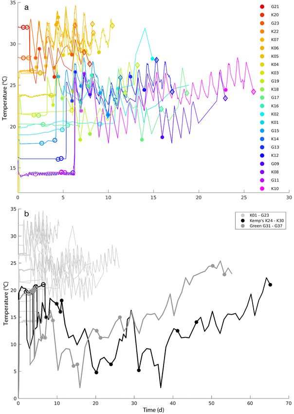
32                                        Endang Species Res 47: 29–47, 2022

appropriate conditions. Carcass condition and tem-           (‘deployment carcasses’; Reneker et al. 2018). Here,
perature were recorded twice daily, in the morning           we briefly summarize the relevant methods from this
and evening on most days. Carcass condition was              work, which included a notable sample size.
recorded using the following previously developed               The time and temperature required to float was
criteria based on the degree of bloating and percent-        determined for 104 cold-stunned sea turtle carcasses
age of the carcass above the waterline: Code 2.1, first      (78 green sea turtles and 26 Kemp’s ridleys) used for
floating; 2.2, moderate bloat; 3.1, fully bloated (i.e.      drift experiments. During calendar year 2017, these
peak floating); 3.2, post bloat; 3.3, sinking; 4, heavily    carcasses were systematically thawed in holding
decomposed; and 5, bare bones (Reneker et al. 2018;          tanks at near 20−25°C for up to 3 d until they first
see the Appendix). In order to ensure that our back-         floated, then maintained near 18°C until used in drift
tracking method is applicable to general sea turtle          experiments (Reneker et al. 2018). Time−temperature
stranding data, we also applied a more general car-          histories were recorded on Kestrel Drop digital re-
cass condition classification system used by the             corders at 20 min intervals, then averaged to hourly
STSSN: fresh dead or mildly decomposed (Code 1),             values. These carcasses were not monitored via cam-
moderately decomposed (Code 2), severely decom-              era; therefore, an accurate TTF is unknown. Car-
posed (Code 3), dried carcass (Code 4), and bones            casses were checked every few hours during the day.
(Code 5). Hereafter, coding of decomposition stages          While some were observed floating during the day,
follows Reneker et al. (2018) except when specifi-           others were found floating in the morning. The esti-
cally referred to as STSSN coding.                           mated TTF included greater uncertainty than those
                                                             determined by time-lapse video in the current study;
                                                             however, observations were mostly within 12 h of the
     2.2.6. Accumulated degree hours and modeling            actual TTF and thus still provided a useful range for
                                                             comparison purposes.
   We characterized decomposition using accumulated
degree hours (ADH), which measures thermal energy
input into the carcass during decomposition in order                           2.4. Drift experiments
to standardize temperature on the rate of decomposi-
tion (Cook et al. 2020). ADH values were calculated            The above deployment carcasses were used in car-
by summing the hourly mean water temperatures at             cass drift experiments to understand stranding season-
each stage of decomposition beginning when a car-            ality (Cook et al. 2021). For the current study, we en-
cass was placed in the tank through its duration in the      hanced a backtrack model based on parameters from
harbor. Although carcasses were exposed to ambient           our decomposition studies and used the drifter experi-
air and water temperatures, only water temperature           ment data to evaluate the ability of the model to predict
was considered relevant when calculating ADH. We             the general location of the drop sites. Drift tracks from
made this choice because water has a much higher             wooden effigies utilized by Cook et al. (2021) were also
specific heat conductivity than air and is the primary       used to evaluate the accuracy of the model. Small, 2’ ×
driver of heat loss or gain in carcasses because they        3’ × 1’ (5.1 × 7.6 × 2.5 cm) SPOT Trace GPS satellite
are always at least 50% submerged. As presented in           transmitters (SPOT) provided real-time monitoring of
Section 3, we found that the relationship between            locations and determination of the actual time objects
temperature, ADH, and decomposition was nonlinear,           reached land or if they were lost at sea.
i.e. carcasses decomposed much faster when ADH                 A total of 182 carcasses and 100 effigies, hereafter
was accrued at higher temperatures, thus we also             referred to as ‘objects,’ were deployed at 3 sites (A, B,
derived a corrected ADH (cADH) that incorporated             C), twice per month during the 2017 drift study (Cook
this temperature dependence (Text S1).                       et al. 2021). To maximize comparability of effigies
                                                             and carcasses, only effigies with drift durations that
                                                             did not exceed observed carcass decomposition rates
                2.3. Comparative data                        were selected for backtracking. Only 46% (n = 120)
                                                             of objects were included in the analysis. The remain-
  To corroborate findings from the tank and carboy           ing objects either vanished (possible scavenging or
experiments, we compared these results with those            decomposition of carcasses or SPOT malfunction),
from a previously published study in which de-               were effigies that drifted beyond the persistence of
composed carcasses were deployed and tracked in              an actual carcass, or were objects that were never
the Gulf of Mexico to study carcass drift and fate           recovered (Cook et al. 2021). Over half (n = 63) of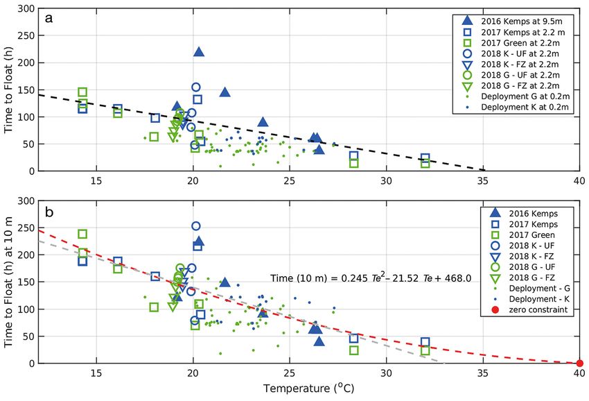
Nero et al.: Turtle carcass decomposition and backtracking                                 33

beached objects were deployed from inshore Site A,            carcasses were maintained in the harbor until they
followed by 39 at intermediate Site B, and 18 from            sank and only bare bones remained; however, 4
offshore Site C (Cook et al. 2021).                           carcasses (K03, K08, G09, and G14) were lost prior
   Predicted condition codes were calculated for effi-        to becoming skeletonized due to either human in-
gies (n = 59) by first estimating the cADH at beach-          terference or breaching of the sea pens by scav-
ing. To do this, the cADH to float (cADHf ) for each          engers. Fig. 1 provides a detailed example of a time−
deployment site was calculated using deployment               temperature sequence of a single carcass (K04), from
depth and bottom temperature obtained from NOAA               freshly thawed (Day 0), through first floating (3.7 d),
Northern Gulf Ocean Forecast System (NGOFS) and               sinking (9 d), and then decomposition to bare bones
Eqs. (2) & (3), defined in Section 3.1. This value was        (10.5 d). Temperature and time data, presented in a
then added to the result of the sea surface temper-           similar way as for K04 above (Fig. 1), are shown for
ature at deployment multiplied by the number of               the first 23 trials conducted during the warmer spring
hours adrift to calculate the total predicted cADH at         and summer months (Fig. 2a), where each carcass is
beaching. A condition code was then assigned to the           represented by a unique color, ranked by their initial
effigy by comparing its predicted beaching cADH               temperature, from warmest (G21) to coolest (K10).
and the mean cADH for each condition code, derived            TTF, peak float (90−100% of carapace exposed
from our carcass studies, and assigning it to the clos-       above the waterline, severely bloated, > 3/4 of head
est code (Cook et al. 2021). Carcass decomposition            and neck visible above waterline), time to sink, and
codes were also evaluated. If the carcass deployment          bare bones are indicated as symbols on each line
condition code was 2.1 or 2.2 (n = 44), the actual            (Fig. 2a). Generally, the warmest trials decomposed
beaching condition code when found was assigned.              the fastest, being complete in 5−10 d, while the
However, if the deployment condition code was 3.1             coolest trials took up to 25 d.
(n = 20), due to difficulties achieving carcass flota-          The final group of 14 carcasses used in the frozen
tion, then the beaching condition code was also pre-          versus unfrozen experiments (Cook et al. 2020),
dicted in the same way as the effigies.                       was tested during winter months because of the
   Backtrack modeling was carried out using the mod-          limited availability of fresh carcasses at other times.
eling algorithms described in Eqs. 1−11
in Section 3 and the numerical meth-
ods described by Nero et al. (2013),
who downloaded oceanographic data
from the NGOFS hydrodynamic model
(https://tidesandcurrents.noaa.gov/ofs/
ngofs/ngofs.html), with 15 min linearly
interpolated time steps within the
NGOFS hourly resolution. NGOFS is a
40-layer finite element model providing
high resolution (200−300 m scale)
within the complex coastal bays and
estuaries out to a coarse resolution (~5−
10 km scale) near the outer boundary of
the model at the shelf edge. All compu-
tations were carried out using Matlab
(The Math Works).

             3. RESULTS

  3.1. Decomposition experiments
                                            Fig. 1. Time−temperature observations of decomposition trial number 4 (Kemp’s
     3.1.1. TTF and temperature             ridley K04), from the tank in 2016. Red circles and line: YSI-85 Handheld Dis-
                                            solved Oxygen, Conductivity, Salinity and Temperature System measurements;
                                            blue line: Seamon time−depth recorder (TDR) measurements; green line: best
 Tank and carboy experiments pro-           fit of YSI and TDR data as used in the analysis. Vertical dashed lines designate
duced the TTF for 37 carcasses. Most             observations of the time of float, sink, and decomposition to bare bones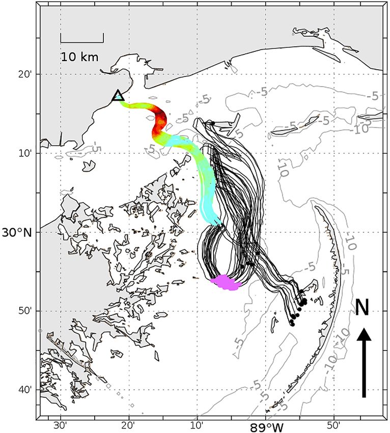
34                                            Endang Species Res 47: 29–47, 2022

Fig. 2. (a) Summary of 23 decomposition trials with: 7 Kemp’s ridley carcasses in the tank (K01−K07) and 16 carcasses in the
carboy, of which 8 were Kemp’s ridleys (K08−K22, even numbers), and 8 were green sea turtles (G09−G23, odd numbers).
Line colors designate the approximate overall mean temperature at which experiments were initially conducted, ranging from
cool (purple−blue) to warm (red). Open circles designate time of floating, asterisks mark peak float, filled circles indicate sink-
ing, and diamonds represent the bare bones stage. (b) Summary of 14 additional cold-temperature decomposition trials shown
on an extended time scale with: 7 Kemp’s ridley carcasses (black curves) and 7 green sea turtle carcasses (medium grey).
           Marker symbols as in panel (a) but with the first 23 carcasses (warmer trials) in light grey to reduce clutter
Nero et al.: Turtle carcass decomposition and backtracking                                  35

Because of their longer duration in the harbor,                                   3.1.2. Temperature effect
these turtles are presented as sets of additional
time−temperature curves in Fig. 2b. Since all 7                      The influence of temperature on decomposition
carcasses of each group (Kemp’s ridley or green                    and resulting TTF is apparent in the plot of the TTF
sea turtle), were placed simultaneously into the                   against the average temperature recorded during
carboy and then eventually all ended up in the                     each experiment (Fig. 3a). In all cases, temperature
harbor, the time−temperature curves for each group                 was relatively stable over the length of each experi-
in Fig. 2b are nearly identical. In this second group              ment because of the controlled conditions in the tank
(Fig. 2b), the TTF at 20°C ranged from 2 to 6 d, but               and carboy. The data show a strong reduction in TTF
decomposition to sinking was extremely long,                       at higher temperatures, with carcasses at near 20°C
requiring an additional 50 to 60 d because of the                  taking ca. 90 h to float, and carcasses maintained
exceptionally cold temperatures in the harbor. Al-                 near 30°C taking about 30 h. A simple linear regres-
though decomposition rates varied between species,                 sion was fit to the data to give a relationship of TTF
there was overlap between species and also notable                 to temperature for the 37 experimental carcasses
variability within species (Cook et al. 2020), and                 (Fig. 3a).
the mean carcass size (Kemp’s ridley = 27.2 cm                       In order to apply the relationship in Fig. 3a in a
straight carapace length [SCL], green = 26.2 cm                    backtracking model system, 2 problems must be ad-
SCL) was not significantly different (p = 1.000)                   dressed: (1) above 35°C, the linear regression falls
between species; therefore, the results of all the                 below 0 h; and (2) there is a tendency for the carcasses
carcasses were treated as 1 set of 37 observations                 maintained at 9.5 m to have a greater TTF than those
in subsequent analysis.                                            at 2.2 m and shallower. The latter prediction is logical

Fig. 3. Observed time to float (TTF) for 37 decomposition trials. (a) TTF at various depths. Black dashed line is a simple linear
regression fit to the data, showing the relationship of TTF to temperature. (b) TTF extrapolated to a depth of 10 m. Least
squares 2nd-order polynomial fit to the experimental trial data is represented by a red dashed line. The red dot marks the zero
constraint point, i.e. the value through which the polynomial regression was constrained. The grey dashed line is the linear re-
gression fit of TTF on temperature (Te) for the experimental trial data from (a). M: Kemp’s ridley in the 2016 tank trials;
H: Kemp’s ridley in the 2017 carboy trials; H: green sea turtles in the 2017 carboy trials; Y: 2018 frozen Kemp’s ridley; S: 2018
unfrozen Kemp’s ridley; Y: 2018 frozen green sea turtles; S: 2018 unfrozen green sea turtles; •: deployment Kemp’s ridley;
                                                 •: deployment green sea turtles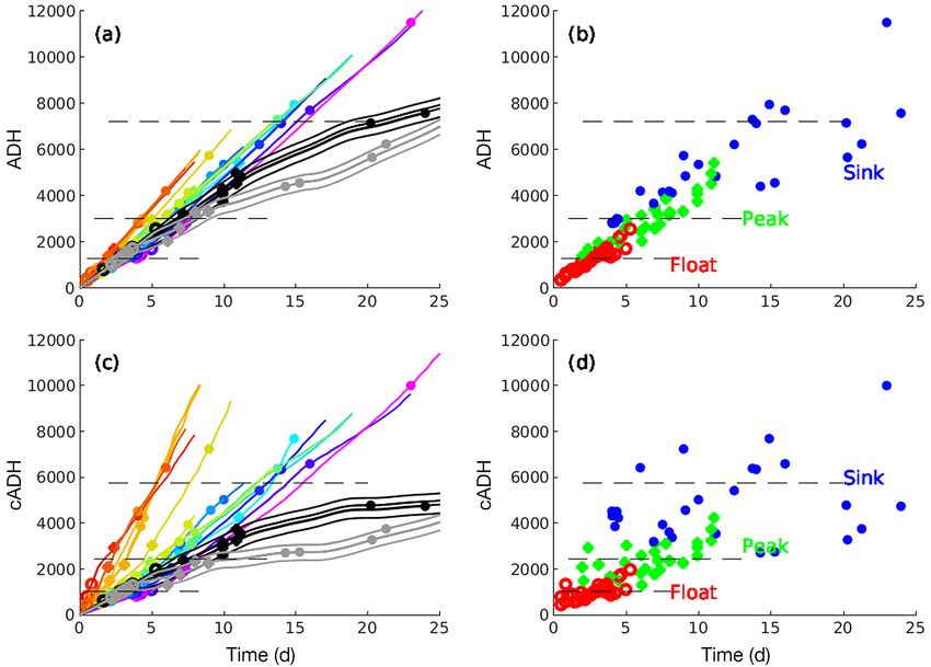
36                                       Endang Species Res 47: 29–47, 2022

based on Boyle’s law where gas produced by decom-           izing the TTF for all 37 carcasses to 20°C (in ad-
position at about 10 m would occupy a volume half           dition to the 10 m depth criteria). We found a pos-
that occupied at 0 m. Addressing these backtrack            sible difference (p = 0.1, t-test) with green sea tur-
model problems required examining this likely pres-         tles showing a quicker TTF than the Kemp’s ridleys.
sure effect more closely.                                   However, as evident in the overlap of the data
                                                            in Fig. 3b, this is not a strong difference and for
                                                            the purpose of modeling, the 2 species are treated
                3.1.3. Pressure effect                      identically.

   The spread of the residuals about the linear
regression of the TTF shows that carcasses in the            3.1.4. Decomposition: comparing ADH and cADH
tank at 9.5 m (K1−K7) took up to 2 times longer to
float than the other 30 carcasses at depths less than         The integration of temperature with time, as ADH,
2.2 m at the same temperature (Fig. 3a). Comparison         is shown in Fig. 4a for the 37 carcass trials where
of residuals with the Mann-Whitney test gave a low          each carcass is shown as a trajectory line, gaining
probability (p = 0.01) that this occurrence was by          degree hours as time progresses. Also shown are 3
chance alone and led us to conclude that the depar-         measures of the mean ADH for critical stages of
ture of the carcasses at 9.5 m depth (K1−K7), from          decomposition related to carcass drift denoted as:
the results for the 30 carcasses maintained at 2.2 m,       ‘Float’ (Code 2.1), ‘Peak’ or maximum buoyancy
was primarily due to the influence of the greater           (Code 3.1), and ‘Sink’ when the carcass sank beneath
pressure at 9.5 m, in this case 1.22 atm, versus            the surface (Code 3.3). A scatter of the ADH values of
1.95 atm, a factor of 1.6×.                                 each stage about their means is shown in Fig. 4b.
   Based on a likely pressure effect on the TTF, the        There was a trend of increasing ADH with time
influence of pressure was compensated using Boyle’s         within each stage due to high temperatures having a
law to adjust all TTF to a standard depth, in this case     greater influence on decomposition (Fig. 4a). Car-
a depth of 10 m. This calculation assumed that ambi-        casses maintained at high temperatures trend along
ent pressure is directly proportional to gas produc-        trajectories towards the left side of Fig. 4a, reaching
tion and the TTF. Fig. 3b provides a re-plotting of the     a given stage sooner, while carcasses kept at cool
37 experimental measurements of TTF as calibrated           temperatures trend towards the right-hand side, tak-
to a standard depth of 10 m. With all carcasses plot-       ing much longer. The result is that an equal value of
ted using the pressure-adjusted TTF, a nonlinear            ADH will give different results that are dependent on
decrease in TTF is evident in the relationship of tem-      the actual ambient temperature. The overall effect is
perature to TTF (Fig. 3b). A polynomial regression          that 1 h decomposing at 30°C causes far more de-
(see Text S1 for derivation) with a zero constraint at      composition than 2 h at 15°C. Thus, the ADH is not
40°C fit the pressure adjusted data for the 37 experi-      successfully independent from temperature and does
mental carcasses as:                                        not sufficiently predict stage of decomposition based
                                                            on ambient temperature alone.
      TTF(10 m) = 0.246Te2 – 21.52Te + 468.0        (1)
                                                              To account for the nonlinear increase in decom-
  The zero constraint ensures that no values pre-           position observed at higher temperatures, we de-
dicted by the regression would fall below zero. This        rived a cADH. Numerical detrending, in this case
polynomial is the basis of a quantitative model of          dividing ADH by the polynomial expressing time
time for carcasses to float based on water tempera-         from temperature, gives a temperature correction
ture and is employed in fitting a general model of          (Tc) as:
carcass decomposition using the units of ADH. Since                                     2086.4
the TTF is a quantitative measure of decomposition,                   Tc =                                      (2)
                                                                              0.246Te 2 − 21.52Te + 468.0
the relationship of Ratkowsky et al. (1983) is then
used in detrending the decomposition rate from tem-         where 2086.4 is the rotation point on which the
perature (see Text S1) where it can be employed to          detrending occurs. This point was chosen as the mid-
integrate the environmental temperature (Te) over           point at 25°C for the range of temperatures, 18−32°C,
widely varying conditions using the cADH.                   that are expected when applying the decomposition
  The polynomial regression (Eq. 1) also allows for         model in the northern Gulf of Mexico.
a test of any difference in TTF between species,              The ADH values for decomposition stages were
Kemp’s ridley versus green sea turtles, by standard-        replotted using the cADH as defined in Eq. (2)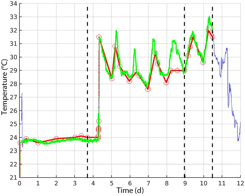
Nero et al.: Turtle carcass decomposition and backtracking                                  37

Fig. 4. Accumulated degree hours (ADH) over time (days) for the 37 experimental trials. Horizontal dashed lines indicate the
mean values of time to float (Float), maximum bloat (Peak), and time of sinking (Sink). (a) Curve colors matched to initial
experimental trials as per Fig. 2. (b) ADH for trials as in panel (a), but with curves removed and symbols plotted in 1 color for
each time to float (red), maximum bloat (green), and time of sinking (blue). (c) Corrected ADH (cADH) for trials, with symbols
          and colors as in panel (a). (d) cADH for trials, with curves and symbols simplified for clarity as in panel (b)

(Fig. 4c,d). Under this calculation, cADH accumulate                                 3.1.6. TTF calculation
much more quickly at the higher temperatures and
at reduced rates at the cooler temperatures. Fig. 4d                 As expected based on field observations, car-
also demonstrates how the temperature depend-                      casses used in this study sank and required some
ency of the decomposition is better incorporated                   amount of decomposition and accumulation of gas
into the calculation of the cADH as evidenced by                   to float (Figs. 1 & 2a,b). At 1 atm (essentially the sea
a more uniform distribution around their mean                      surface), a carcass will float once it has reached
values for each stage of floating/sinking.                          cADHf = 1014.9 degree hours (see Text S1), but at
                                                                   greater depths, a higher value is required (greater
                                                                   pressure at depth). The cADH to float (cADHf) at a
        3.1.5. Decomposition codes and cADH                        specific depth (Z) can be calculated as:

   cADH values for decomposition codes are shown                                                        (
                                                                                  cADHf(Z ) = cADHf 1 + Z
                                                                                                        10      )            (3)
in Fig. 5. Mean values and incremental values be-
tween each code are annotated on the plot. Al-                       Incorporating the influence of the corrected tem-
though somewhat cluttered, the curves linking the                  perature (Tc), TTF can be calculated as:
cADH for each carcass provide a more uniform
measure of decomposition than uncorrected ADH,
                                                                                   TTF =
                                                                                         cADHf 1 + Z(
                                                                                                   10       )                (4)
i.e. without correcting for temperature. Based on
                                                                                             Tc
condition code evident at the time of stranding, the
corresponding mean cADH value can be used in                         The result of Eq. (4) will be the TTF (h) for a carcass
backtrack calculations.                                            that immediately sank after death.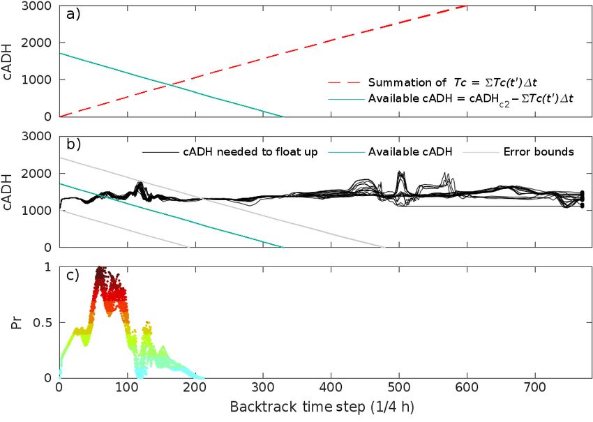
38                                          Endang Species Res 47: 29–47, 2022

                                                                                 and assume decomposition at these
                                                                                 stages is related to temperature in the
                                                                                 same way as it was for the TTF. We
                                                                                 also measured ADH requirements for
                                                                                 carcasses to reach STSSN codes 2 and
                                                                                 3, although not as precisely deter-
                                                                                 mined as the TTF (under camera sur-
                                                                                 veillance) since judging these codes is
                                                                                 more subjective and only monitored
                                                                                 about every 12 h. Data suggest much
                                                                                 faster decomposition at high tempera-
                                                                                 tures as noted with other codes.

                                                                                      3.2.2. Backtracking formula

                                                                                    We applied the above relationships
                                                                                 to determine the likely position along
                                                                                 a backtrack route where a carcass
                                                                                 most likely originated, i.e. death oc-
Fig. 5. Corrected accumulated degree hours (cADH) for all experimental car-      curred. We use STSSN code 2 as an
casses extending from carcass condition codes 2.1 through 5 (see the Appen-
                                                                                 example, but STSSN code 3 can be
dix for code descriptions). Bold numbers at the top of the curves and × symbols
on the plot are the mean cADH to achieve each level of condition code, lighter   calculated similarly. Only STSSN
numbers are the net cADH between condition codes. Curve colors are those         codes 2 and 3 are used for back-
                                 used in Fig. 2a                                 tracking. While code 1 (fresh dead or
                                                                                 mildly decomposed) could be used, in
                 3.2. Backtrack modeling                           many instances carcasses in this condition strand
                                                                   alive and die on the beach and may not have been
  3.2.1. Integration of carcass parameters as applied              passively drifting as carcasses do. In addition, the
                  in the backtrack model                           postmortem interval of carcasses classified as codes
                                                                   4 and 5 is highly uncertain rendering backtracking
   Carcass decomposition and the eventual production               results unreliable. Those carcasses found as desic-
of gas, vg, is a function of the environmental tempera-            cated or skeletal remains could have drifted a great
ture as corrected for decomposition, Tc (see Text S1),             distance or may have been discovered days after
and accumulates as a function of time, t. dt is the dif-           beaching.
ferential of time t. Integration of vg(Tc(t)) from death             The effect of ocean temperature can be used in a
at t = 0 to the time that a carcass floats to the surface,         degree-hour budget and deducted from the avail-
t = TTF, can be represented as the integration:                    able degree-hours of a carcass along the backtrack
                             TTF                                   route as:
                  cADHf = ∫ vg (Tc (t ))dt                 (5)
                                                                               cADH(t') = cADHc 2 − ∑ Tc (t')Δt      (8)
                           0
giving the cADH to float, cADHf.                                 The left-hand term is the cADH along the back-
  Once a carcass reaches the sea surface (at TTF), it          track route at time t ’, used here to designate the
continues to decompose, and subsequent stages of               reverse time steps implemented for the backtrack-
decomposition can also be measured as the contin-              ing, Δt is the time interval used for the back-
ued integration of decomposition from the moment of            tracking. The cADHc2 is the total cADH an STSSN
death to each later stage, as an STSSN code 2 (c2)             code 2 carcass would have accumulated upon its
and 3 (c3) respectively as:                                    arrival on shore. The right-hand summation term
                           2                                   is the summation of the temperature correction,
               cADHc 2 = ∫ vg (Tc (t ))dt              (6)     Tc, along the backtrack route. When Eq. (8) solves
                           0                                   to zero, i.e. the cADH on shore is equal to the
                           3
               cADHc 3 = ∫ vg (Tc (t ))dt              (7)     Tc summed along the backtrack route, then the
                           0                                   maximum backtrack location is achieved at which
Nero et al.: Turtle carcass decomposition and backtracking 39
the carcass would most likely have originated 3.3. Individual backtrack example
had it not initially sunk to the sea floor (i.e. the
cADH = 0). Carcass backtracking from beach stranding loca-
As mentioned above, at 1 atm (essentially the sea tions provides at-sea estimates of where death might
surface), a carcass will float once it has reached have occurred. Nero et al. (2013) used ocean model-
cADHf = 1014.9 degree hours (Fig. 5), but at greater generated estimates of surface currents and winds,
depths a higher value will be required (greater pres- as well as the leeway, to directly determine the
sure at depth). In backtracking, an adjustment for along-track coordinates, and a final endpoint based
actual depth (and pressure) on the sea floor is neces- on a preset number of time steps. However, no con-
sary. Since varying depths are found along the back- sideration was given for ocean depth and the time
track route, we apply Boyle’s law along the back- required for a carcass to decompose and generate
track route as: enough gas to float to the sea surface. Furthermore,
(
cADHf( Z (t')) = cADHf 1 +
Z (t')
10 ) (9)
no consideration was given for the possibility that
carcasses in deep water might not resurface. To
over depths Z and time steps t ’, to determine the demonstrate the new set of routines, outlined above
cADHf for locations on the track line. (Eqs. 2−11), an example backtrack is given below
When the backtracked budget for a carcass, and 2 additional examples are provided in the sup-
cADH(t’), Eq. (8) equals the depth-compensated plemental material (Text S2).
Boyle’s law in cADHf(Z(t ’)), Eq. (9), we then have A sea turtle was found on the beach as an STSSN
an exact match for a backtrack location that is code 2 carcass on 1 May 2019 in Waveland, Missis-
solved for both the temperature along the surface sippi. The model first uses the ocean model currents
route and the influence of water depth on the TTF of and winds from NGOFS to backtrack for 192 h (8 d)
a carcass as: in time (Fig. 6) in the same way as per Nero et al.
(2013). The 192 h provides a reverse time sequence
cADH(t’) – cADHf(Z(t’)) = 0 (10)
The calculation of Eq. (10) is critical in solving
backtracks since there are variations in water depth
along the backtrack route, such as with deep bays
and offshore shoals. In these cases, a decomposed
carcass could originate from shallower depths further
offshore, or possibly deeper depths close to shore.
There may also be deep offshore locations, well
beyond 30−40 m, from which the carcass likely could
not originate. Thus, Eq. (10) may give more than one
solution. When the solution is not perfect, but close,
this information can also be used as an indicator of
goodness of fit.
Since the actual measurements of carcass decom-
position show considerable variation in the TTF and
the cADH, we can use this variability to introduce
error bounds to estimate uncertainty in comparing
Eqs. (8) & (9) and provide a method of comparing
the various solutions along the backtrack route. The
error ranges for the STSSN code 2 and code 3 car-
casses are: E2 = 709 cADH and E3 = 827 cADH,
respectively. Probable locations of origin, Pr, for a
carcass along its backtrack route (t’) can then be
determined as:
(
Pr (t') =
E )
E − |cADH(t') − cADHf(Z (t'))| 2
(11)
Fig. 6. Backtrack of a beach-stranded Sea Turtle Stranding
and Salvage Network (STSSN) code 2 carcass; beach loca-
tion is designated with a triangle. Individual lines are the
where a value of 1 indicates a perfect fit, and con- ensemble of 20 random backtrack realizations produced
versely lower values tending towards zero indicate a using a 10% random walk with black dots representing the
poor fit and low likelihood. furthest track endpoints40 Endang Species Res 47: 29–47, 2022
sufficient to give an appropriate track
length for most STSSN code 2 car-
casses found in the northern Gulf of
Mexico, while STSSN code 3 car-
casses require 288 h, or 12 d.
Solving to determine where along
the length of the backtrack (Fig. 6)
that mortality most likely occurred
is complicated, as it is dependent on
both water temperature and pressure
(depth). Bathymetry data provide bot-
tom depth (Fig. 7a) and the ocean
model output used for the backtrack-
ing can be simultaneously queried to
provide estimates of the surface tem-
perature (Fig. 7b, Te). Bottom depth is
applied in Eq. (9) to determine the
cADHf for various positions on the
predicted track line (Fig. 7b, Tc).
The temperature conversion for-
mula, Eq. (2), is then used to convert Fig. 7. Conditions along the backtrack route for a sea turtle found on the beach
the sea surface temperature along the as an STSSN code 2 carcass on 1 May 2019 in Waveland, MS. (a) Bathymetry, (b)
temperature at the sea surface along the backtrack route (Te) and its conversion
backtrack route, Te, into the form re-
to the corrected temperature (Tc), and (c) bathymetry converted to corrected
quired for the decomposition calcula- accumulated degree hours (cADH) required to float along the backtrack route
tions, Tc (Fig. 7b). In early May, the
22−24°C temperatures were calculated
to 18−22°C temperatures, and also de-
clined with time at earlier points along
the backtrack (Fig. 7b). They also show
a 24 h sawtooth pattern, the influ-
ence of the day−night heating−cooling
cycle.
The cumulative sum of Tc along the
backtrack (Fig. 8a) is then subtracted
from the total cADH of the carcass as
found on the beach (cADHc2) as in
Eq. (8), giving the resulting cADH
for positions on the backtrack route
(Fig. 8a). This curve begins at the
beach, with time step 0, at 1723 cADH,
and gradually declines to 0 cADH at
about time step 330, (equivalent to
83 h, or 3.4 d). This decline to zero
cADH is the likely timestep when the Fig. 8. (a) Calculation of the cumulative sum of Tc along the backtrack route
sea turtle may have died had it begun (red dashed line). The subtraction of the cADH along the backtrack from the
drifting without ever sinking to the sea starting value of the ADH for an STSSN code 2 carcass found on the beach
(cADHc2) giving the net budget of available cADH at each point along the
floor. If the carcass was categorized as
backtrack route is shown as a teal line. (b) An overlay of the cADH budget
an STSSN code 3 upon stranding, a along the backtrack (teal line) with the cADH necessary for a carcass to float
cADHc3 of 3258 would be applied. up from the sea floor (black curves) as well as the ± error bounds on the cADH
For carcasses that sink, the proba- budget (thin lines). The process to calculate the cADH necessary for a carcass
to float up from the sea floor is shown in Fig. 7. (c) Resulting probability of ori-
ble locations of origin are then deter-
gin values created from comparing the above cADH curves in (a) using Eq. (11)
mined by comparing the cADH and described in Section 3 for backtracking. Colors range from low probability
cADHf curves, as in Eq. (10), and (light blue) to high probability (dark red)Nero et al.: Turtle carcass decomposition and backtracking 41
shown graphically in Fig. 8b. Where the cADHf and persistence of carcasses. Although there have been
error curves cross, calculated using Eq. (10), are the numerous studies on human (Mateus & Pinto 2016,
backtrack time steps most likely to have been the Reijnen et al. 2018) and animal decomposition (An-
locations of origin for the carcass, i.e. where death derson & Hobischak 2004, Anderson & Bell 2014,
occurred. The solution of Eq. (11), which calculates 2016), few researchers have studied decomposition
the squared relative difference, then provides a of marine animals or sea turtles in particular (Santos
probability, or likelihood estimate, as shown in Fig. et al. 2018). Using cadaver studies and robust sam-
8c, from 0 (low) to 1 (high). The likelihood values are ple sizes, we show that both depth and water tem-
then co-located using the along-track latitude−longi- perature significantly influence sea turtle decom-
tude data to color map the original backtrack plots position, which has considerable bearing on the
(Fig. 9). One optional feature for the map plots is to dispersal of dead sea turtles and thus probability of
provide estimates of the possible source locations if discovery.
the carcasses had never sunk. These locations are The time required for a submerged carcass to float
shown as the purple points in Fig. 9. is a key measurement for mortality investigation. For
sea turtles that sink upon death, as has been noted
for important mortality sources such as fisheries
3.4. Drift experiments bycatch, the TTF identifies the first instance that a
carcass reaches the sea surface, is influenced by sur-
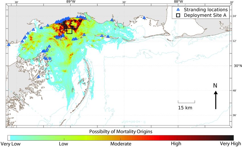
Backtrack heatmaps of predicted source locations face winds and oceanic currents, and is visible for
for the objects released at the 3 deployment sites discovery. Fortunately, it is also the most quantifiable
(Cook et al. 2021) are shown in Figs. 10−12. The and least subjective parameter observed during our
backtracking model predicted the original deploy- decomposition trials, despite the potential for consid-
ment locations at Sites A and B with high probability erable variation due to species, body composition,
(Figs. 10 & 11, respectively). This outcome suggests and diet (Cook et al. 2020). We found a significant
that if carcasses were from an actual sea turtle mor- depth/pressure and temperature effect; TTF was
tality event, the model would accurately estimate the
general area where sea turtles died. Backtracking of
Site B objects centered on the deployment site while
the region of high probability was just slightly
inshore of Site A. Backtracking of Site C objects,
which incidentally required longer time periods and
distances (Fig. 12), was less accurate than the more
inshore sites (Figs. 10 & 11).
4. DISCUSSION
Mortality of animals in the marine environment is
by its nature often cryptic. Marine animals found on
shore, i.e. stranded, present formidable challenges to
biologists, wildlife managers, and other scientists
who seek to understand mortality sources. These
issues are particularly acute for imperiled species
where strandings can generate considerable concern
among stakeholders and resource agencies, as well
as influence mitigation measures and other conser-
vation actions. Determining the location where a
marine animal actually died is often a critical ques-
tion, as it may help link mortality with specific causes
or circumstances. Predicting locations of mortality Fig. 9. Resulting probability of origin for a carcass back-
tracked from a beach location (triangle). Probability color
sources requires understanding of both taphonomic range as in Fig. 8c, with addition of the possible carcass
processes and the environmental factors that influ- source if having never sunk (purple dots) and backtrack
ence decomposition, as well as the dispersal and endpoints (black dots)42 Endang Species Res 47: 29–47, 2022
Fig. 10. Backtracking heat map generated for 63 objects (carcasses and wood block effigies) systematically deployed in 2017
from Site A (black square in the middle of Mississippi Sound) and object ‘stranding’ or beaching locations (blue triangles) in
coastal Mississippi and eastern Louisiana. Heat map colors range from zero probability (white), through low (light blue) to
high (dark red to black)
Fig. 11. As in Fig. 10, but for 39 objects (carcasses and wood block effigies) deployed from Site B (black square) just south of
Ship IslandNero et al.: Turtle carcass decomposition and backtracking 43
Fig. 12. As in Fig. 10, but for 18 objects (carcasses and wood block effigies) deployed from Site C (black square) in offshore
waters of Mississippi
longer when incubated at colder temperatures and ~4000 cADH) or they will never float. At this stage,
greater depths. The TTF followed an inverse curvi- the carcass likely loses its structural integrity to the
linear relationship where carcasses exposed to the degree that it can no longer contain internal gases.
coldest temperatures took 8× longer to float. The car- Extrapolation of the TTF of 1014.95 cADH suggests
casses used for drift studies also illustrated this pres- this depth is between 30 and 40 m. However, temper-
sure effect. They were kept in small coolers (~20 cm ature will also influence how long it takes for a carcass
depth) and were the quickest to float (dots in Fig. 3a to become buoyant; therefore, outcome likely depends
that are well below the line) because they were at on both depth and associated temperatures. Our pre-
sea level. In the northern Gulf of Mexico, Kemp’s rid- diction seems consistent with parameters applied to
ley sea turtles commonly occupy habitat from near- submerged human bodies. The National Underwater
shore waters ≤ 37 m to offshore regions of 50−60 m Rescue-Recovery Institute states that humans that
and are observed in depths up to 200 m (Shaver & drown in −1 to 4°C water will not surface unless the
Rubio 2008, Coleman et al. 2017). Green sea turtles water temperature increases. They also state that
primarily occupy nearshore, shallow waters, but will 30 m is likely the depth at which pressure and tem-
frequent deeper water seasonally or during migration perature cause a body to never surface (J. Sanders et
(Hart & Fujisaki 2010, Shaver et al. 2013). Sea turtles al. unpubl. data). This concept is inherent in the appli-
have been found in water temperatures as low as cation of Eq. (9) and our backtracking model.
10°C, or colder depending on species (Epperly et al. There are several important considerations with
1995); thus a broad range of water temperatures and regard to our experimental findings and comparisons
depths is relevant to studies of sea turtle mortality. with the natural fate of sea turtle carcasses in the
Beyond certain depth and temperature thresholds, environment. While the majority of our experiment
a carcass will not generate enough gases to overcome was conducted in field conditions, the initial TTF
the influences of pressure, temperature, and volume occurred in a controlled laboratory setting, and thus
to float to the surface. We hypothesize that submerged some factors such as scavenging were not accounted
carcasses must generate enough gas and float before for. We assume that opportunity for scavenging by
they become severely decomposed (condition 3.3 at benthic fauna and resulting damage to the carcass44 Endang Species Res 47: 29–47, 2022 increases with TTF duration. If a carcass is subjected of sea turtles that die from sudden causes, accounts to heavy scavenging and conditions result in a long of turtles sinking upon death, limited data acquired TTF, it could become compromised to the degree that from sea turtles that died while carrying actively it cannot hold gases and never floats. Similarly, car- transmitting satellite-enabled tags, and the general casses restrained underwater, such as those entan- characteristics of strandings in our region (Nero et al. gled in ghost fishing gear or other submerged debris, 2013). Aforementioned conditions in which sea tur- would never reach the surface. While these possibil- tles strand alive or float upon death require addi- ities should be considered in any analysis of strand- tional interpretation and assumptions, which are ings and broader at-sea mortality, the focus of our accommodated by the model’s flexibility (Fig. 9). research and model application was investigative The set of routines used in the model allow the tools to study carcasses that wash ashore. incorporation of time, temperature, and bathymetry Potential differences in decomposition and buoy- into the backtrack modeling of sea turtle carcasses. ancy among sea turtle species and sizes are addi- The use of TTF, as adjusted by pressure and temper- tional considerations. Our calculations are based on ature to resolve the uncertainty in the backtracks, data derived from Kemp’s ridley and green sea tur- provides an innovative solution to estimating the at- tles; however, TTF and decomposition rates would sea origin of sea turtle mortalities. Our test of the likely follow similar patterns for other species, espe- model accuracy predicted the source location of year- cially those of similar size. Sea turtles used to create round deployments of 120 sea turtle effigies and car- equations were 21.1−31.6 cm SCL due to carcass casses, demonstrating the overall reliability of the availability and the predominant size distribution of model. The model is also able to predict the source stranded sea turtles in the region of study. Sutherland location for carcasses that do not sink by taking the et al. (2013) compared decomposition rates of large reversed cADH and searching that array for where and small pigs in a terrestrial environment. Initial de- they reach zero. These carcasses begin drifting imme- composition rates were similar for all sizes, although diately, which results in longer drift tracks. The re- larger carcasses decomposed slower during the ad- duced ability of the model to predict drifts with longer vanced stages of decomposition. Overall, smaller pig durations of 3−4 d, and distances of 40−50 km from carcasses decomposed nearly 3 times faster and did shore likely reflect the additive role of random and not follow the same rate of progression as the larger small-scale (sub-model scale space and time) sea and pig carcasses (Sutherland et al. 2013). If sea turtles weather conditions, as well as decreasing the ability of follow the same trend, it is possible that TTF predic- the NGOFS ocean model to give reliable backtracks tions would not be impacted since floating occurs over increasing time periods and steps that are inher- in the initial decomposition process and only latter ent to longer predictions. Nonetheless, we feel that the stages would vary. However, the factors influencing resulting model and application are very useful, partic- the decomposition process on land and in the marine ularly for mortality within 10 km of shore, given that environment are very different due to the absence of drifting test objects came ashore over a wide region of insect activity. Santos et al. (2018) included 2 larger coastal Mississippi and eastern Louisiana (~4000 km2). sea turtle carcasses (67 and 68 cm) in addition to 6 The conversion of temperature to the cADH rather smaller sea turtles (26−37 cm) in their decomposition than simply using ADH is essential to our approach study, and did not notice a size effect. However, the because the exact reverse time−temperature history coarse time resolution of their observations (days) of carcasses found on the beach cannot be deter- may have masked size-related differences. Future mined until the backtrack trajectory, temperature decomposition studies with larger sea turtles are history, and projected depth of origin are resolved. In required to truly understand if body size significantly the model, a corrected temperature was used, which affects decomposition and buoyancy of sea turtles. made the ADH estimate independent of actual tem- Our carcass studies provide valuable additional perature. If the routines were rewritten to use a tem- data on sea turtle decomposition, but our ultimate perature-dependent ADH value for each condition objective was to characterize key postmortem pro- code, the predicted mortality location could be erro- cesses in order to parameterize the backtracking neous if changes in temperature and depth condi- model. Several aspects of our approach should be tions occur along the backtrack. considered with regard to use in mortality investiga- A few key conditions of our backtracking model tion. First, our focus was the postmortem scenario in must be considered, including the need to document which carcasses initially sink and become buoyant the actual time of stranding and accurately charac- with decomposition based on our interest in the fate terize postmortem condition when a carcass first
Nero et al.: Turtle carcass decomposition and backtracking                               45

comes ashore. For these reasons, we only apply the             lite-tagged Kemp’s ridley drifted 1.4 km between its
model in areas of regular human use or structured              final transmission before death and its resurfacing
shoreline surveys for stranded sea turtles where both          5 d later. The Argos location class errors could also
time of stranding and postmortem condition can be              account for some discrepancy in location just before
confidently ascertained. Photographs and informa-              death as these can range up to 1.5 km or potentially
tion related to discovery must be carefully reviewed           greater (CLS 2016). In addition, we have monitored
to ensure that data inputs are sufficient for back-            42 sea turtle carcasses placed on the seafloor in non-
tracking. Currently, the STSSN does not record the             anchored cages in the northern Gulf of Mexico as
actual time when the carcass was first discovered,             part of additional decomposition studies and have
which can introduce error into the model. To account           observed very limited movement (E. Schultz pers.
for the range of possible times when the carcass may           obs.). Thus, we do not feel that subsurface drift
have beached on the day it was reported, the model             majorly influences carcass dispersal in this region,
is run at five 6 h intervals (0, 6, 12, 18, and 24) to pro-    but should be considered if this model is applied in
duce a spaghetti plot of possible drift tracks.                regions where stronger bottom currents occur.
   Backtracking accuracy also relies on accurate as-              In conclusion, we provide time−temperature rela-
signment of postmortem condition code upon strand-             tionships for stages of decomposition and key post-
ing, which requires careful validation. While carcasses        mortem events that are relevant to backtracking of
are floating, decomposition rates are driven primarily         dead stranded sea turtles in order to predict the area
by water temperature because water has a higher                where they died. The intent of this work is to provide
specific heat conductivity than air. However, once             the best possible estimates of mortality source loca-
carcasses beach, sunlight and the temperature of the           tions using ocean models as described by Nero et al.
sand can greatly affect decomposition rates. During            (2013) and enhanced with ambient pressure derived
summer months, if a carcass is not found within hours          from ocean bathymetry and corrected temperature.
of beaching, it will quickly decompose, which typi-            Our approach may be adapted to other regions where
cally results in a longer drift track than would be pre-       suitable ocean circulation models are available. As in
dicted if carcass condition was determined when it             the northern Gulf of Mexico, we encourage the use of
first came ashore. As with time of stranding, confi-           appropriate drifter studies to evaluate model per-
dence in condition code upon stranding may simply              formance.
be too uncertain for application in remote or irregu-
larly surveyed locations. To overcome these issues,
                                                               Acknowledgements. We thank the many staff and volun-
the model can be run using a range of input parame-            teers from the Massachusetts, Mississippi, Texas, and North
ters (i.e. times, condition codes) for circumstances           Carolina Sea Turtle Stranding and Salvage Network (STSSN)
where lesser degrees of confidence are still useful.           for salvaging and shipping carcasses during several seasons
                                                               (2016, 2017, and 2018). Without their dedication and re-
   Currently, only sea turtles with condition codes 1,
                                                               sponse effort this study would not have been possible. We
2, or 3 are simulated in the model to ensure the most          also thank the staff and patrons of the Bay-Waveland Yacht
accurate outputs. It is not possible to accurately esti-       Club for the use of their facility. This research was sup-
mate the mortality location for a dried carcass or             ported with Sea Turtle Early Restoration Project funds
skeletal remains because the postmortem interval is            administered by the Deepwater Horizon Natural Resource
                                                               Damage Assessment Regionwide Trustee Implementation
potentially very long and too uncertain. Also, we              Group. Sea turtle research was authorized under DOI
developed the parameters of our model based on                 USFWS TE 676395-5 issued to the Southeast Fisheries
postmortem condition classification criteria currently         Science Center (PI: Dr. Bonnie J. Ponwith) and USFWS
used by the STSSN in order to maximize applicabil-             designated agent letter issued to M.C. This study was also
                                                               partially supported by NOAA National Centers for Environ-
ity; however, a more detailed system of carcass cate-          mental Information and NOAA grant 363541-191001-
gorization described by Reneker et al. (2018) provides         021000 (Northern Gulf Institute) at Mississippi State Univer-
more highly resolved backtrack calculations and bet-           sity. Mention of trade names or commercial companies is for
ter estimates of likely at-sea mortality locations.            identification purposes only and does not imply endorse-
                                                               ment by the National Marine Fisheries Service, NOAA.
   An additional factor that may be significant in
some regions is bottom drift, which is not incorpo-
rated into our model. Evidence from research in the                               LITERATURE CITED
northern Gulf of Mexico suggests that bottom drift
                                                               Anderson GS, Bell LS (2014) Deep coastal marine taphon-
plays a minimal role in overall carcass movement as              omy: investigation into carcass decomposition in the
compared to wind and current forcing at the sea sur-             Saanich Inlet, British Columbia using a baited camera.
face. Nero et al. (2013) found that a deceased satel-            PLOS ONE 9:e110710
You can also read