Cross-scale interaction of host tree size and climatic water deficit governs bark beetle-induced tree mortality - USDA Forest Service
←
→
Page content transcription
If your browser does not render page correctly, please read the page content below
ARTICLE
                  https://doi.org/10.1038/s41467-020-20455-y                 OPEN

                  Cross-scale interaction of host tree size and
                  climatic water deficit governs bark beetle-induced
                  tree mortality
                  Michael J. Koontz 1,2,3 ✉, Andrew M. Latimer                          1,2,   Leif A. Mortenson4, Christopher J. Fettig5 &
                  Malcolm P. North1,2,6
1234567890():,;

                  The recent Californian hot drought (2012–2016) precipitated unprecedented ponderosa pine
                  (Pinus ponderosa) mortality, largely attributable to the western pine beetle (Dendroctonus
                  brevicomis; WPB). Broad-scale climate conditions can directly shape tree mortality patterns,
                  but mortality rates respond non-linearly to climate when local-scale forest characteristics
                  influence the behavior of tree-killing bark beetles (e.g., WPB). To test for these cross-scale
                  interactions, we conduct aerial drone surveys at 32 sites along a gradient of climatic water
                  deficit (CWD) spanning 350 km of latitude and 1000 m of elevation in WPB-impacted Sierra
                  Nevada forests. We map, measure, and classify over 450,000 trees within 9 km2, validating
                  measurements with coincident field plots. We find greater size, proportion, and density of
                  ponderosa pine (the WPB host) increase host mortality rates, as does greater CWD. Criti-
                  cally, we find a CWD/host size interaction such that larger trees amplify host mortality rates
                  in hot/dry sites. Management strategies for climate change adaptation should consider how
                  bark beetle disturbances can depend on cross-scale interactions, which challenge our ability
                  to predict and understand patterns of tree mortality.

                  1 Graduate Group in Ecology, University of California, Davis, CA, USA. 2 Department of Plant Sciences, University of California, Davis, CA, USA. 3 Earth Lab,

                  University of Colorado-Boulder, Boulder, CO, USA. 4 USDA Forest Service, Pacific Southwest Research Station, Placerville, CA, USA. 5 USDA Forest Service,
                  Pacific Southwest Research Station, Davis, CA, USA. 6 USDA Forest Service, Pacific Southwest Research Station, Mammoth Lakes, CA, USA.
                  ✉email: michael.koontz@colorado.edu

                  NATURE COMMUNICATIONS | (2021)12:129 | https://doi.org/10.1038/s41467-020-20455-y | www.nature.com/naturecommunications                                    1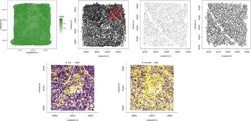
ARTICLE                                                                 NATURE COMMUNICATIONS | https://doi.org/10.1038/s41467-020-20455-y

B
       ark beetles dealt the final blow to many of the nearly 150              forests are more prone to bark beetle-induced tree mortality
       million trees killed in the California hot drought of                  compared to thinned forests6,9, which may arise as greater
       2012–2016 and its aftermath1. A harbinger of climate                   competition for water resources amongst crowded trees lowers
change effects to come, record high temperatures exacerbated the              average tree resistance31, or because smaller gaps between trees
drought2,3, which increased water stress in trees4,5, making them             protect pheromone plumes from dissipation by the wind and thus
more susceptible to colonization by bark beetles6,7. Further, a               enhance intraspecific beetle communication32. Tree size is
century of fire suppression has enabled forests to grow into dense             another aspect of forest structure that affects bark beetle host
stands, which can also make them more vulnerable to bark                      selection behavior with smaller trees tending to have a lower
beetles6,8,9. This combination of environmental conditions and                capacity for resisting attack, but larger trees being more desirable
forest structural characteristics led to tree mortality events of             targets on account of their thicker phloem providing greater
unprecedented size across the state10,11.                                     nutritional content13,33–35. Throughout an outbreak, some bark
   Tree mortality exhibited a strong latitudinal and elevational              beetle species will collectively “switch” the preferred size of the
gradient4,11 that can only be partially explained by coarse-scale             tree to attack in order to navigate this trade-off between host
measures of environmental conditions (i.e., historic climatic water           susceptibility and host quality13,21,36–39. Taking forest composi-
deficit; CWD) and current forest structure (i.e., current regional             tion alone, WPB activity in the Sierra Nevada mountain range of
basal area)11. A progressive loss of canopy water content offers              California is necessarily tied to the regional distribution of its
additional insight into tree stress and mortality risk, but cannot            exclusive host, ponderosa pine18. Colonization by primary bark
ultimately resolve which trees are actually killed by bark beetles or         beetles can also depend on the local relative frequencies of tree
elucidate factors driving bark beetle population dynamics and                 species in forest stands, reflecting the more general pattern that
spread5. Bark beetles respond to local forest characteristics in              specialist insect herbivory tends to be lower in taxonomically
positive feedbacks that non-linearly alter tree mortality dynamics            diverse forests compared to monocultures40,41.
against a background of environmental conditions that stress                     The interaction between forest structure and composition at
trees12,13. Thus, explicit consideration of local forest structure and        both stand- and tree-scales also drives WPB activity. For instance,
composition14,15, as well as its cross-scale interaction with                 dense forest stands with high host availability may experience
regional climate conditions16, can refine our understanding of                 greater beetle-induced tree mortality because dispersal distances
tree mortality patterns from California’s recent hot drought. The             between potential host trees are shorter, which reduces predation
challenge of simultaneously measuring the effects of both local-              of adults searching for hosts and facilitates higher rates of
scale forest features (such as structure and composition) and                 colonization33,42,43. High host availability can also reduce the
broad-scale environmental conditions (e.g., CWD) on forest                    chance of individual beetles wasting their limited resources flying
insect disturbance leaves their interaction effect relatively                 to and landing on a non-host tree44,45. At a finer scale, a host
underexplored14–17.                                                           tree’s defensive capacity can depend on its canopy position, with
   The ponderosa pine/mixed-conifer forests in California’s Sierra            reduced biochemical defenses in suppressed, crowded trees46.
Nevada region are characterized by regular bark beetle dis-                   Coarse-scale measures of forest structure and composition can
turbances, primarily by the influence of western pine beetle                   therefore only partially explain mechanisms affecting bark beetle
(Dendroctonus brevicomis; WPB) on its host ponderosa pine                     disturbance. Finer-grain information is also needed that explicitly
(Pinus ponderosa)18. WPB is a primary bark beetle—its repro-                  recognizes tree species, size, and local density, which better cap-
ductive success is contingent upon host tree mortality, which                 tures the ecological processes underlying insect-induced tree
itself requires enough beetles to mass attack the host tree and               mortality28,36,38,39.
overwhelm its defenses19. This Allee effect creates a strong cou-                The vast spatial extent of WPB-induced tree mortality in the
pling between beetle selection behavior of host trees and host tree           2012–2016 California hot drought challenges our ability to
susceptibility to colonization19–21. A key defense mechanism of               simultaneously consider how broad-scale environmental condi-
conifers to bark beetle attack is to flood beetle boreholes with               tions may interact with local forest structure and composition
resin, which physically expels colonizing beetles, can be toxic to            to affect the dynamic between bark beetle selection and coloni-
the colonizers and their fungi, and may interrupt beetle                      zation of host trees, and host tree susceptibility to attack15,47.
communication22,23. Under normal conditions, weakened trees                   Measuring local forest structure generally requires expensive
with compromised defenses are the most susceptible to coloni-                 instrumentation4,48 or labor-intensive field surveys14,15,49, which
zation and will be the main targets of primary bark beetles like              constrains survey extent and frequency. Small, unhumanned
WPB13,23,24. Under severe water stress, however, many trees no                aerial systems (sUAS) enable relatively fast and cheap remote
longer have the resources available to mount a defense7,13.                   imaging over hundreds of hectares of forest, which can be used to
Drought12,25–27,     especially     when      paired      with    high        measure complex forest structure and composition at the indi-
temperatures24,28–30, can trigger increased bark beetle-induced               vidual tree scale with Structure from Motion (SfM)
tree mortality as average tree vigor declines. As the local popu-             photogrammetry50,51. The ultra-high, centimeter-scale resolution
lation density of beetles increases due to successful reproduction            of sUAS-derived measurements, as well as the ability to incor-
within spatially aggregated susceptible trees, mass attacks grow in           porate vegetation reflectance, can help overcome challenges in
size and become capable of overwhelming formidable tree                       species classification and dead tree detection inherent in other
defenses. Even large healthy trees may be susceptible to coloni-              remote sensing methods, such as airborne LiDAR52. Distributing
zation and mortality when beetle population density is                        such surveys across an environmental gradient can overcome the
high13,23,24. Thus, water stress and beetle population density                data acquisition challenge inherent in investigating phenomena
interact to influence whether individual trees are susceptible to              with both a strong local- and a strong broad-scale component.
bark beetles. When extreme or prolonged drought increases host                   We used sUAS-derived remote sensing images over a network
tree vulnerability, bark beetle population growth rates increase,             of 32 sites in Sierra Nevada ponderosa pine/mixed-conifer forests
then become self-amplifying as greater beetle densities make                  spanning 1000 m of elevation and 350 km of latitude14 covering a
additional host trees prone to successful mass attack12,13,15,24.             total of 9 km2, to investigate how broad-scale environmental
   WPB activity is strongly influenced by forest structure—the                 conditions interacted with local forest structure and composition
spatial arrangement and size distribution of trees—and tree spe-              to shape patterns of tree mortality during the cumulative tree
cies composition. Taking forest structure alone, high-density                 mortality event of 2012 to 2018. We asked:

2                NATURE COMMUNICATIONS | (2021)12:129 | https://doi.org/10.1038/s41467-020-20455-y | www.nature.com/naturecommunications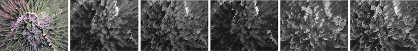
NATURE COMMUNICATIONS | https://doi.org/10.1038/s41467-020-20455-y                                                                                                                  ARTICLE

 Table 1 Correlation and differences between the best-performing tree detection algorithm (lmfx with dist2d = 1 and ws = 2.5)
 and the ground data.

 Forest structure metric                                Ground mean                           Correlation with ground                        RMSE                     Median error
 Total tree count                                       19                                    0.67*                                           8.68*                   2
 Count of trees >15 m                                   9.9                                   0.43                                            7.38                    0
 Distance to 1st neighbor (m)                           2.8                                   0.55*                                           1.16*                   0.26
 Distance to 2nd neighbor (m)                           4.3                                   0.61*                                           1.70*                   0.12
 Height (m); 25th percentile                            12                                    0.16                                            8.46                    −1.2
 Height (m); mean                                       18                                    0.29                                            7.81*                   −2.3
 Height (m); 75th percentile                            25                                    0.35                                           10.33*                   −4

 An asterisk next to the correlation or RMSE indicates that this value was within 5% of the value of the best-performing algorithm/parameter set. Ground mean represents the mean value of the forest
 metric across the 110 field plots that were visible from the sUAS-derived imagery. The median error is calculated as the median of the differences between the air and ground values for the 110 visible
 plots. Thus, a positive number indicates an overestimate by the sUAS workflow and a negative number indicates an underestimate.

  1. How does the proportion of the ponderosa pine host trees                                          Effect of local structure and regional climate on tree mortality
     in a local area and average host tree size affect WPB-                                            attributed to WPB. Site-level CWD exerted a positive main effect
     induced tree mortality?                                                                           on the probability of ponderosa mortality (effect size: 0.85; 95%
  2. How does the density of all trees (hereafter “overall                                             CI: [0.70, 0.99]; Fig. 1). We found a positive main effect of the
     density”) affect WPB-induced tree mortality?                                                      proportion of host trees per cell (effect size: 0.68; 95% CI: [0.62,
  3. How does the total basal area of all trees (hereafter “overall                                    0.74]), with a greater proportion of host trees (i.e., ponderosa
     basal area”) affect WPB-induced tree mortality?                                                   pine) in a cell increasing the probability of ponderosa pine
  4. How does environmentally driven tree moisture stress                                              mortality. We detected no effect of overall tree density or overall
     affect WPB-induced tree mortality?                                                                basal area (i.e., including both ponderosa pine and non-host
  5. How do the effects of forest structure, forest composition,                                       species; tree density effect size: −0.01; 95% CI: [−0.11, 0.08];
     and environmental condition interact to influence WPB-                                             basal area effect size: −0.13; 95% CI: [−0.29, 0.03]).
     induced tree mortality?                                                                              We found a positive two-way interaction between the overall
   Here, we show that a greater local proportion of host trees                                         tree density per cell and the proportion of trees that were hosts,
(ponderosa pine) strongly increases the probability of host mor-                                       which is equivalent to a positive effect of the density of host trees
tality, with greater host density amplifying this effect. We also                                      (effect size: 0.06; 95% CI: [0.01, 0.12]; Fig. 1).
show that greater site-level CWD increases host mortality                                                 We found a positive main effect of the mean height of
rates. Further, we show that larger host trees increase the prob-                                      ponderosa pine on the probability of ponderosa mortality (effect
ability of host mortality in accordance with the well-known life                                       size: 0.25; 95% CI: [0.14, 0.35]). Coupled with the strong
history of WPB. Critically, we find a strong interaction between                                        correlation between the proportion of dead host trees and basal
host size and CWD such that host mortality rates are especially                                        area killed (Supplementary Fig. 1 and Supplementary Note 1),
high in hot/dry sites where the local average host tree size is large.                                 these results suggest that WPB-attacked larger trees, on average.
Our results demonstrate a cross-scale interaction in the response                                      Further, there was a strong positive interaction between CWD and
of WPB to local forest structure and composition across an                                             ponderosa pine mean height, such that larger trees were especially
environmental gradient, which helps reconcile differences                                              likely to increase the local probability of ponderosa mortality in
between observed ecosystem-wide tree mortality patterns and                                            hotter, drier sites (effect size: 0.54; 95% CI: [0.37, 0.70]; Fig. 2).
predictions from models based on coarser-scale forest structure.                                          We found no effect of the site-level CWD interactions with the
                                                                                                       proportion of host trees (effect size: −0.08; 95% CI: [−0.18, 0.03])
                                                                                                       or of the interaction between CWD and total basal area (effect
Results                                                                                                size: −0.04; 95% CI: [−0.23, 0.15]; Fig. 1).
Tree detection algorithm performance. We found that the                                                   We found a negative effect of the CWD interaction with overall
experimental lmfx algorithm53 with parameter values of dist2d =                                        tree density (effect size: −0.19; 95% CI: [−0.31, −0.07]) as well as
1 and ws = 2.5 performed the best across seven measures of forest                                      of the interaction between the mean height of host trees and the
structure as measured by Pearson’s correlation with ground data                                        overall basal area (effect size: −0.08; 95% CI: [−0.13, −0.03];
(Table 1).                                                                                             Fig. 1).
                                                                                                          While we found no interaction between the proportion of host
Classification accuracy for live/dead and host/non-host. The                                            trees and mean host tree height, we did find a 3-way interaction
accuracy of live/dead classification on a withheld testing data set                                     between these variables with CWD (effect size: 0.14; 95% CI:
was 96.4%. The accuracy of species classification on a withheld                                         [0.04, 0.24]; Fig. 1).
testing data set was 64.1%. The accuracy of WPB host/non-WPB-
host (i.e., ponderosa pine versus other tree species) on a withheld                                    Discussion
testing data set was 71.8%.                                                                            This study uses drone-derived imagery to refine our under-
                                                                                                       standing of the patterns of tree mortality following the 2012 to
Site summary based on best tree detection algorithm and                                                2016 California hot drought and its aftermath. By simultaneously
classification. Across all study sites, we detected, segmented, and                                     measuring the effects of local forest structure and composition
classified 452,413 trees in 23,187, 20 × 20 m pixels (with the area                                     across broad-scale environmental gradients, we were able to
of each pixel being approximately equivalent to that of a field                                         better characterize the influence of a tree-killing insect, the WPB,
plot). Of these trees, we classified 118,879 as dead (26.3% mor-                                        compared to using correlates of tree stress alone.
tality). Estimated site-level tree mortality ranged from 6.8% to
53.6%. See Supplementary Table 1 for site summaries and com-                                           Strong positive main effect of CWD. We found a strong positive
parisons to site-level mortality measured from field data.                                              effect of site-level CWD on ponderosa pine mortality rate. We did

NATURE COMMUNICATIONS | (2021)12:129 | https://doi.org/10.1038/s41467-020-20455-y | www.nature.com/naturecommunications                                                                                    3
ARTICLE                                                                                              NATURE COMMUNICATIONS | https://doi.org/10.1038/s41467-020-20455-y

                                                                                         Intercept
                                                                                        Site CWD
                                                                       Proportion host (ponderosa)
                                                                           Ponderosa mean height
                                                                                   Overall density
                                                                                Overall basal area
                                                           Site CWD : Proportion host (ponderosa)
                                                               Site CWD : Ponderosa mean height
                                                                        Site CWD : Overall density
                                                                     Site CWD : Overall basal area
                                                    Proportion host (ponderosa) : Overall density
                      Proportion host (ponderosa) : Ponderosa mean height
                                                        Ponderosa mean height : Overall basal area
             Site CWD : Proportion host (ponderosa) : Ponderosa mean size

                                                                                                            −0.5             0.0          0.5              1.0
                                                                                                                            Effect size
                                                                                                            Log odds change in Pr(Ponderosa mortality)
                                                                                                          for a 1 standard deviation increase in covariate
Fig. 1 Posterior distributions of effect size from zero-inflated binomial model predicting the probability of ponderosa pine mortality in a 20 × 20-m cell
given forest structure characteristics and site-level climatic water deficit (CWD). The gray filled area for each model covariate represents the probability
density of the posterior distribution, the point underneath each density curve represents the median of the estimate, the bold interval surrounding the point
estimate represents the 66% credible interval, and the thin interval surrounding the point estimate represents the 95% credible interval. Estimates for all
model parameters, including Gaussian Process parameters for each site, can be found in Supplementary Table 2.

                                                              cool/wet site             average site               hot/dry site
                       Pr(ponderosa mortality)

                                                 0.75

                                                                                                                                      Mean
                                                                                                                                      host tree
                                                                                                                                      height
                                                 0.50
                                                                                                                                           Larger trees
                                                                                                                                           Smaller trees

                                                 0.25

                                                        −1.0 −0.5 0.0 0.5 1.0−1.0 −0.5 0.0 0.5 1.0−1.0 −0.5 0.0 0.5 1.0
                                                                Proportion host trees (Ponderosa pine); scaled
Fig. 2 Line version of model results with 95% credible intervals showing the primary influence of ponderosa pine structure on the probability of
ponderosa pine mortality, and the interaction across climatic water deficit. The “larger trees” line represents the mean height of ponderosa pine
0.7 standard deviations above the mean (approximately 24.1 m), and the “smaller trees” line represents the mean height of ponderosa pine 0.7 standard
deviations below the mean (~12.1 m).

not measure tree water stress at an individual tree level as in other                                    does not allow us to disentangle whether water availability was
recent work15, and instead treated CWD as a general indicator of                                         lower in an absolute sense during the drought or whether
tree stress following results of coarser-scale studies11. When                                           increasing tree vulnerability to bark beetles was driven by chronic
measured at a fine scale, even if not at an individual tree level,                                        water stress at these historically hotter/drier sites54.
progressive canopy water loss can be a good indicator of tree
water stress and increased vulnerability to mortality from drought
or bark beetles5. Though our entire study area experienced                                               Positive effect of host proportion and density. A number of
exceptional hot drought between 2012 and 20162,3, using a 30-                                            mechanisms associated with the relative abundance of species in a
year historic average of CWD as a site-level indicator of tree stress                                    local area might underlie the strong effect of host proportion on

4                  NATURE COMMUNICATIONS | (2021)12:129 | https://doi.org/10.1038/s41467-020-20455-y | www.nature.com/naturecommunications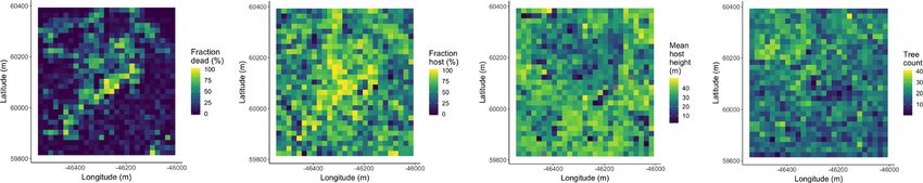
NATURE COMMUNICATIONS | https://doi.org/10.1038/s41467-020-20455-y                                                                    ARTICLE

the probability of host tree mortality. Frequency-dependent her-                found no main effect of overall basal area on the probability of
bivory—whereby mixed-species forests experience less herbivory                  ponderosa mortality, nor of its interaction with site-level CWD.
compared to monocultures (as an extreme example)—is com-                        This contrasts with the results from Young et al.11, and from
mon, especially for oligophagous insect species40. Non-host                     analyses of coincident field plots14. While the contrast to Young
volatiles reduce the attraction of several species of bark beetles              et al.11 might be explained by different scales of analyses (i.e.,
to their aggregation pheromones55, including WPB56. Combina-                    3500 × 3500 m pixels vs. 20 × 20 m pixels), the contrast with the
tions of non-host volatiles and an anti-aggregation pheromone                   coincident ground plots is more puzzling. One explanation is that
have been used successfully to reduce levels of tree mortality                  the drone sampling captured more area beyond the conditionally
attributed to WPB in California57,58. The positive relationship                 sampled field plots (i.e., 10% ponderosa pine basal area mortality
between host density and susceptibility to colonization by bark                 was a criterion for plot selection) that reflected a different rela-
beetles has been so well-documented at the experimental plot                    tionship between local basal area and tree mortality. Perhaps
level43,59,60 that lowering stand densities through the selective               more likely is that our measure of the total basal area is not
harvest of hosts is commonly recommended for reducing future                    precise enough to represent the local competitive environment
levels of tree mortality attributed to bark beetles61, including                compared to the field-derived basal area. For our study, the basal
WPB18. Greater host density shortens the flight distance required                area was derived from species-specific and inherently noisy
for WPB to disperse to new hosts, which likely facilitates bark                 allometric relationships with tree height, which itself was derived
beetle spread, however, we calibrated our aerial tree detection to              from the SfM processing of drone imagery. As remote sensing
~400 m2 areas rather than to individual tree locations, so our data             technology improves to enable finer-scale information extraction
are insufficient to address these relationships. Increased density of            (e.g., individual tree measurements), more dialog between ecol-
ponderosa pine, specifically, may disproportionately increase the                ogists of all stripes65–67 is needed to fully imagine how to best
competitive environment for host trees (and thus increase their                 measure natural phenomena remotely, either by adopting wheels
susceptibility to WPB colonization) if intraspecific competition                 already invented (e.g., plot basal area) or by innovating something
amongst ponderosa pine trees is stronger than the interspecific                  brand new.
competition as would be predicted with coexistence theory62.
Finally, greater host densities increase the frequency that
                                                                                Positive main effect of host tree mean size. The positive main
searching WPB land on hosts, rather than non-hosts, thus
                                                                                effect of host tree mean size on ponderosa mortality rates tracks
reducing the amount of energy expended during host finding and
                                                                                the conventional wisdom on the dynamics of WPB in the Sierra
selection as well as the time that searching WPB spend exposed to
                                                                                Nevada, as well as other primary bark beetles18. WPB exhibits a
a variety of predators outside the host tree.
                                                                                preference for trees 50.8–76.2 cm DBH68,69, and a positive rela-
                                                                                tionship between host tree size and levels of tree mortality
No main effect of overall density, but interaction with CWD.                    attributed to WPB was reported by Fettig et al.14 in the coincident
We detected no relationship between overall tree density and                    field plots as well as in other recent studies9,15,70. Larger trees are
ponderosa pine mortality, though work from the coincident                       more nutritious and are therefore ideal targets if local bark beetle
ground plots showed a negative but weak relationship when using                 density is high enough to successfully initiate mass attack and
proportion of trees killed as a response14. Kaiser et al.28 also show           overwhelm tree defenses, as can occur when many trees are under
greater mountain pine beetle (Dendroctonus ponderosae) infes-                   water stress7,13,24. In the recent hot drought, we expected that
tation in lower-density sites in Montana However, Hayes et al.31                most trees would be under severe water stress, setting the stage
and Fettig et al.14 found that measures of overall tree density                 for increasing beetle density, successful mass attacks, and tar-
explained more variation in tree mortality than measures of host                geting of larger trees. Given that our dead tree height calibration
availability, though those conclusions were based on broader-                   was conservative (accounting for underestimates of drone-derived
scale analyses31 or a different response variable (i.e., “total                 dead tree heights relative to field-measured trees), it is likely that
number of dead host trees”14 rather than a binomial response of                 the positive main effect of tree height that we report represents a
“number of dead host trees conditional on the total number of                   lower bounds of this effect. Additionally, Fettig et al.14 found no
host trees” as in our study).                                                   tree size/mortality relationship for incense cedar or white fir in
   Our greater sample size may have enabled us to more finely                    the coincident field plots. These species represent 22.3% of the
parse the role of multi-faceted forest structure and composition,               total tree mortality observed in their study, yet in our study, all
along with CWD and interactions, in driving ponderosa pine                      dead trees were classified as ponderosa pine (see “Methods”
mortality rates. Indeed, we did find a negative two-way                          section), which could have further dampened the positive effect of
interaction between site CWD and overall density, suggesting                    tree size on tree mortality that we identified.
denser stands experienced lower rates of ponderosa mortality in
hotter, drier sites, which comports with Restaino et al.9 in results
                                                                                Cross-scale interaction of CWD and host tree size. In hotter,
from their unmanipulated gradient of overall density in the same
                                                                                drier sites, a larger average host size increased the probability of
region during the same hot drought. In the absence of active
                                                                                host mortality. Notably, a similar pattern was shown by Stovall
management, forest structure is largely a product of climate and,
                                                                                et al.65 in a study confined to the southern Sierra Nevada (i.e., the
with increasing importance at finer spatial scales, topographic
                                                                                hottest, driest portion of the more spatially extensive results we
conditions63. Denser forest patches in our study may indicate
                                                                                present here) with a strong positive tree height/mortality rela-
greater local water availability, more favorable conditions for tree
                                                                                tionship in areas with the greatest vapor pressure deficit and no
growth and survivorship, and increased resistance to beetle-
                                                                                tree height/mortality relationship in areas with the lowest vapor
induced tree mortality, especially when denser patches are found
                                                                                pressure deficit. Our work suggests that the WPB was cueing into
in hot, dry sites9,63,64.
                                                                                different aspects of forest structure across an environmental
                                                                                gradient in a spatial context in a parallel manner to the temporal
Effect of overall basal area. While overall tree density is likely an           context noted by Stovall et al.65 and Pile et al.70, who observed
indicator of favorable microsites in fire-suppressed forests, the                that mortality was increasingly driven by larger trees as the hot
overall basal area is a better indicator of the local competitive               drought proceeded and became more severe. A temporal signal of
environment, especially in water-limited forests63,64. However, we              bark beetles attacking larger and larger host trees reflects the

NATURE COMMUNICATIONS | (2021)12:129 | https://doi.org/10.1038/s41467-020-20455-y | www.nature.com/naturecommunications                             5
ARTICLE NATURE COMMUNICATIONS | https://doi.org/10.1038/s41467-020-20455-y
positive feedback between forest structure and bark beetle Some uncertainty surrounded our ability to detect trees using
population dynamics as the population phase cycles from ende- the geometry of the dense point clouds derived with SfM. The
mic to epidemic13. This positive feedback leading to eruptive horizontal accuracy (i.e., longitude/latitude position) of the tree
population dynamics is well-documented as a temporal phe- detection was better than the vertical accuracy (i.e., height), which
nomenon, and here we show a similar pattern in a spatial context may result from a more significant error contribution by the field-
mediated through site-level CWD. based calculations of tree height compared to tree position
A key difference from the endemic-to-epidemic positive relative to plot center (Table 1). Height measurements were
feedback noted by Boone et al.13 is that none of our study areas particularly challenging for standing dead trees because SfM can
were considered to be in an endemic population phase by typical fail to produce any points representing narrow, needleless
measures of WPB dynamics31,33. WPB dynamics at all sites were treetops in the resulting dense point cloud. Our conservative
considered epidemic, with >5 trees killed per ha (Supplementary calibration of drone-measured tree heights to field-measured
Table 1). The cross-scale interaction between broad-scale CWD heights strengthened the main effect of CWD on host mortality in
and local-scale host tree size, even amongst populations all in an our model and reversed the effect of host tree height. We report
epidemic phase, highlights the dramatic implications of the that larger host trees increase the probability of host tree
positive feedback for landscape-scale tree mortality. The massive mortality, while models using uncalibrated tree heights show that
tree mortality in hotter/drier Sierra Nevada forests (lower latitudes larger trees decrease host mortality rates (see Supplementary
and elevations4,11) during 2012 to 2016 hot drought likely arose as Fig. 3 compared to Fig. 1). While our live/dead classification was
a synergistic alignment of environmental conditions and local fairly accurate (96.4% on a withheld data set), our species
forest structure that allowed WPB to successfully colonize large classifier would likely benefit from better crown segmentation
trees, rapidly increase in population size, and expand. The because the pixel-level reflectance values within each crown are
unexpectedly low mortality in cooler/wetter Sierra Nevada forests averaged to characterize the “spectral signature” of each tree.
compared to model predictions based on coarser-scale forest With better delineation of each tree crown, the mean value of
structure data11 may result from a different WPB response to local pixels within each tree crown will likely be more representative of
forest structure due to a lack of an alignment with favorable that tree’s spectral signature.
climate conditions and a weaker positive feedback. Better tree detection, crown segmentation, and dead tree height
measurement would likely improve with better SfM point clouds
which can be enhanced with greater overlap between images71 or
Limitations and future directions. We have demonstrated that with oblique (i.e., off-nadir) imagery72. Frey et al.71 found that
drones can be effective means of collecting forest data at multiple, 95% overlap was preferable for generating dense point clouds in
vastly different spatial scales to investigate a single, multi-scale forested areas, and James and Robson72 reduced dense point
phenomenon—from meters in between trees, to hundreds of cloud errors using imagery taken at 30 degrees off-nadir. We only
meters of elevation, to hundreds of thousands of meters of lati- achieved 91.6% overlap with the X3 RGB camera and 83.9%
tude. Some limitations remain but can be overcome with further overlap with the multispectral camera, and all imagery was nadir-
refinements in the use of this tool for forest ecology. Most of these facing. We anticipate that computer vision and deep learning will
limitations arise from the classification and measurement of also prove helpful in overcoming some of these detection and
standing dead trees, making it imperative to work with field data classification challenges73.
for calibration and uncertainty reporting. Finally, we note our study is constrained by the uncertainty in
The greatest limitation in our study arising from classification measuring basal area from SfM processing of drone-derived
uncertainty is in the assumption that all dead trees were imagery. This uncertainty makes it challenging to represent
ponderosa pine, which we estimate from coincident field plots typical field-based measures of the local competitive environment
is true ~73.4% of the time. Because the forest structure factors (e.g., total plot basal area) or ecosystem impact (e.g., the
influencing the likelihood of individual tree mortality during the proportion of dead basal area in a plot) in statistical analysis.
hot drought depended on tree species15, we cannot rule out that Instead, we opted to use the probability of ponderosa mortality as
some of the ponderosa pine mortality relationships to forest our key response variable, which is well-suited to understanding
structure that we observed may be partially explained by those the dynamics between WPB colonization behavior and host tree
relationships in other species that were misclassified as ponderosa susceptibility.
pine using our methods. However, the overall community
composition across our study area was similar14 and we are able
to reproduce similar forest structure/mortality patterns in drone- Conclusions. Climate change adaptation strategies emphasize
derived data when restricting the scope of analysis to only trees management action that considers whole-ecosystem responses to
detected in the footprints of the coincident field plots (Supple- inevitable change74, which requires a macroecological under-
mentary Fig. 2). Thus, we remain confident that the patterns we standing of how phenomena at multiple scales can interact. Tree
observed were driven primarily by the dynamic between WPB vulnerability to environmental stressors presents only a partial
and ponderosa pine. While spectral information of foliage could explanation for tree mortality patterns during hot droughts,
help classify living trees to species, the species of standing dead especially when bark beetles are present. We have shown that
trees were not spectrally distinct. This challenge of classifying drones can be a valuable tool for investigating multi-scalar phe-
standing dead trees to species implies that a conifer forest systems nomena, such as how local forest structure combines with
with less bark beetle and tree host diversity, such as mountain environmental conditions to shape forest insect disturbance.
pine beetle outbreaks in relative monocultures of naturally Understanding the conditions that drive dry western U.S. forest
occurring lodgepole pine forests in the Intermountain West, responses to disturbances such as bark beetle outbreaks will be
should be particularly amenable to the methods presented here vital for predicting outcomes from increasing disturbance fre-
even with minimal further refinement because dead trees will quency and intensity exacerbated by climate change75. Our study
almost certainly belong to a single species and have succumbed to suggests that outcomes will depend on interactions between local
colonization by a single bark beetle species. For similar reasons, forest structure and broad-scale environmental gradients, with
these methods would also work particularly well if imagery were the potential for cross-scale interactions to enhance our under-
also captured prior to the mortality event. standing of forest insect dynamics.
6 NATURE COMMUNICATIONS | (2021)12:129 | https://doi.org/10.1038/s41467-020-20455-y | www.nature.com/naturecommunicationsNATURE COMMUNICATIONS | https://doi.org/10.1038/s41467-020-20455-y ARTICLE Fig. 3 The network of field plots spanned a 350-km latitudinal gradient from the Eldorado National Forest in the north to the Sequoia National Forest in the south. Plots were stratified by three elevation bands in each forest, with the plots in the Sequoia National Forest (the southern-most National Forest) occupying elevation bands 305 m above the three bands in the other National Forests in order to capture a similar community composition. Methods and diameter at breast height (DBH) were recorded if DBH was greater than 6.35 Study system. We designed the aerial survey to coincide with 160 vegetation/ cm. The year of mortality was estimated based on needle color and retention if it forest insect monitoring plots at 32 sites established between 2016 and 2017 by occurred prior to plot establishment and was directly observed thereafter during Fettig et al.14 (Fig. 3). The study sites were chosen to reflect typical west-side Sierra annual site visits. A small section of bark (~625 cm2) on both north and south Nevada yellow pine/mixed-conifer forests and were dominated by ponderosa aspects was removed from dead trees to determine if bark beetle galleries were pine14. Sites were placed in WPB-attacked, yellow pine/mixed-conifer forests present. The shape, distribution, and orientation of galleries are commonly used to across the Eldorado, Stanislaus, Sierra, and Sequoia National Forests and were distinguish among bark beetle species18. In some cases, deceased bark beetles were stratified by elevation (914–1219 m, 1219–1524 m, 1524–1829 m above sea level). present beneath the bark to supplement identifications based on gallery formation. In the Sequoia National Forest, the southern-most National Forest in our study, During the spring and early summer of 2018, all field plots were revisited to assess sites were stratified with the lowest elevation band of 1219–1524 m and extended to whether dead trees had fallen14. an upper elevation band of 1829–2134 m to capture a more similar forest com- In the typical life cycle of WPBs, females initiate host colonization by tunneling munity composition as at the more northern National Forests. The sites have through the outer bark and into the phloem and outer xylem where they rupture variable forest structure and plot locations were selected in areas with >35% resin canals. As a result, oleoresin exudes and collects on the bark surface, as is ponderosa pine basal area and >10% ponderosa pine mortality. At each site, five commonly observed with other bark beetle species. During the early stages of the 0.041-ha circular plots were installed along transects with 80–200 m between plots. attack, females release an aggregation pheromone component which, in In the field, Fettig et al.14 mapped all stem locations relative to the center of each combination with host monoterpenes released from pitch tubes, is attractive to plot using azimuth/distance measurements. Tree identity to species, tree height, conspecifics76. An anti-aggregation pheromone component is produced during the NATURE COMMUNICATIONS | (2021)12:129 | https://doi.org/10.1038/s41467-020-20455-y | www.nature.com/naturecommunications 7
ARTICLE NATURE COMMUNICATIONS | https://doi.org/10.1038/s41467-020-20455-y
latter stages of host colonization by several pathways and is thought to reduce Level 3: Domain-specific information extraction
intraspecific competition by altering adult behavior to minimize overcrowding of Level 3a: Data derived from spectral or geometric Level 2 product. Using just the
developing brood within the host77. Volatiles from several non-hosts sympatric spectral information from the radiometrically corrected reflectance maps, we cal-
with ponderosa pine have been demonstrated to inhibit the attraction of WPB to its culated several vegetation indices including the normalized difference vegetation
aggregation pheromones56,78. In California, WPB generally has 2–3 generations in index83 (NDVI; Fig. 4; Level 3a, first image and Supplementary Fig. 13), the
a single year and can often outcompete other primary bark beetles such as the normalized difference red edge88 (NDRE), the red-green index89 (RGI), the red
mountain pine beetle in ponderosa pines, especially in larger trees33. WPB edge chlorophyll index90 (CIred edge), and the green chlorophyll index90 (CIgreen).
population growth rates can, however, be reduced by competition with other beetle Using just the geometric information from the canopy height model or terrain-
species cohabitating in the same host tree, as well as by predation during dispersal normalized dense point cloud, we generated maps of detected trees (Fig. 4; Level 3a,
to seek a host33. second and third images and Supplementary Fig. 14) by testing a total of 7
automatic tree detection algorithms and a total of 177 parameter sets (Table 2). We
used the field plot data to assess each tree detection algorithm/parameter set by
Aerial data collection and processing. Nadir-facing imagery was captured using converting the distance-from-center and azimuth measurements of the trees in the
a gimbal-stabilized DJI Zenmuse X3 broad-band red/green/blue (RGB) camera79 field plots to x–y positions relative to the field plot centers distinguishable in the
and a fixed-mounted Micasense Rededge3 multispectral camera with five narrow Level 2 reflectance maps as the orange fabric X’s that we laid out prior to each
bands80 on a DJI Matrice 100 aircraft81. The imagery was captured from both flight. In the reflectance maps, we located 110 out of 160 field plot centers while
cameras along preprogrammed aerial transects over ~40 ha surrounding each of some plot centers were obscured due to dense interlocking tree crowns or because a
the 32 sites (each of these containing five field plots) and was processed in a series plot center was located directly under a single tree crown. For each of the 110 field
of steps to yield local forest structure and composition data suitable for our sta- plots with identifiable plot centers– the “validation field plots”, we calculated 7
tistical analyses. All images were captured in 2018 during a 3-month period forest structure metrics using the ground data collected by Fettig et al.14: total
between early April and early July, and thus our work represents a postmortem number of trees, number of trees greater than 15 m in height, mean height of trees,
investigation into the drivers of cumulative tree mortality. Following the call by 25th percentile tree height, 75th percentile tree height, mean distance to nearest
Wyngaard et al.82, we establish “data product levels” to reflect the image processing tree neighbor, and mean distance to second nearest neighbor. For each tree
pipeline from raw imagery (Level 0) to calibrated, fine-scale forest structure and detection algorithm and parameter set described above, we calculated the same set
composition information on regular grids (Level 4), with each new data level of 7 structure metrics within the footprint of the validation field plots. We
derived from levels below it. Here, we outline the steps in the processing and calculated the Pearson’s correlation and root mean square error (RMSE) between
calibration pipeline visualized in Fig. 4, and include additional details in the the ground data and the aerial data for each of the 7 structure metrics for each of
Supplementary Methods. the 177 automatic tree detection algorithms/parameter sets. For each algorithm and
parameter set, we calculated its performance relative to other algorithms as to
whether its Pearson’s correlation was within 5% of the highest Pearson’s
Level 0: Raw data from sensors. Raw data comprised ~1900 images per camera
correlation as well as whether its RMSE was within 5% of the lowest RMSE. We
lens (one broad-band RGB lens and five narrow-band multispectral lenses) for each
summed the number of forest structure metrics for which it reached these 5%
of the 32 sites (Fig. 4; Level 0; Supplementary Figs. 4 and 5). Prior to the aerial
thresholds for each algorithm/parameter set. For automatically detecting trees
survey, two strips of bright orange drop cloth (~100 ×15 cm) were positioned as an
across the whole study, we selected the algorithm/parameter set that performed
“X” over the permanent monuments marking the center of the 5 field plots from
well across the most forest metrics (see “Results” section).
Fettig et al.14 (Supplementary Fig. 6).
We delineated individual tree crowns (Fig. 4; Level 3a, fourth image and
We preprogrammed north-south aerial transects using Map Pilot for DJI on
Supplementary Fig. 15) with a marker controlled watershed segmentation
iOS flight software84 at an altitude of 120 m above ground level (with “ground”
algorithm99 implemented in the ForestTools package97 using the detected treetops
defined using a 1-arc-second digital elevation model85). The resulting ground
as markers. If the automatic segmentation algorithm failed to generate a crown
sampling distance was ~5 cm/px for the Zenmuse X3 RGB camera and ~8 cm/px
segment for a detected tree (e.g., often snags with a very small crown footprint), a
for the Rededge3 multispectral camera. We used 91.6% image overlap (both
circular crown was generated with a radius of 0.5 m. If the segmentation generated
forward and side) at the ground for the Zenmuse X3 RGB camera and 83.9%
multiple polygons for a single detected tree, only the polygon containing the
overlap (forward and side) for the Rededge3 multispectral camera.
detected tree was retained. Because image overlap decreases near the edges of the
overall flight path and reduces the quality of the SfM processing in those areas, we
Level 1: Basic outputs from photogrammetric processing. We used SfM pho- excluded segmented crowns within 35 m of the edge of the survey area. Given the
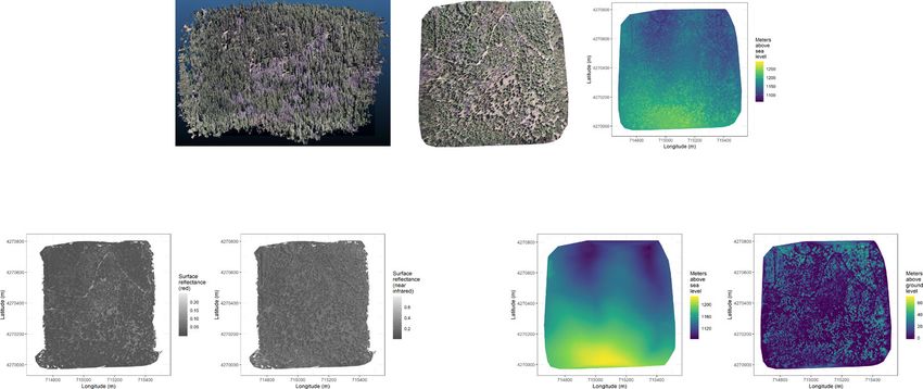
togrammetry implemented in Pix4Dmapper Cloud (www.pix4d.com) to generate narrower field of view of the Rededge3 multispectral camera versus the X3 RGB
dense point clouds (Fig. 4; Level 1, left; Supplementary Fig. 7), orthomosaics (Fig. 4; camera whose optical parameters were used to define the ~40 ha survey area
Level 1, center and Supplementary Fig. 8), and digital surface models (Fig. 4; Level around each site, as well as the 35 m additional buffering, the survey area at each
1, right and Supplementary Fig. 9) for each field site71. For 29 sites, we processed site was ~30 ha (Supplementary Table 1).
the Rededge3 multispectral imagery alone to generate these products. For three
sites, we processed the RGB and the multispectral imagery together to enhance the Level 3b: Data derived from spectral and geometric information. We overlaid the
point density of the dense point cloud. All SfM projects resulted in a single pro- segmented crowns on the reflectance maps from 20 sites spanning the latitudinal
cessing “block,” indicating that all images in the project were optimized and and elevation gradient in the study. Using QGIS (https://qgis.org/en/site/), we hand
processed together. The dense point cloud represents x, y, and z coordinates as well classified 564 trees as live/dead and as one of 5 dominant species in the study area
as the color of millions of points per site. The orthomosaic represents a radio- (ponderosa pine, Pinus lambertiana, Abies concolor, Calocedrus decurrens, or
metrically uncalibrated, top-down view of the survey site that preserves the relative Quercus kelloggi) using the mapped ground data as a guide. Each tree was further
x–y positions of objects in the scene. The digital surface model is a rasterized classified as “host” for ponderosa pine or “non-host” for all other species18. We
version of the dense point cloud that shows the altitude above sea level for each extracted all the pixel values within each segmented crown polygon from the five,
pixel in the scene at the ground sampling distance of the camera that generated the Level 2 orthorectified reflectance maps (one per narrow band on the Rededge3
Level 0 data. camera) as well as from the five, Level 3a vegetation index maps using the velox
package100. For each crown polygon, we calculated the mean value of the extracted
Level 2 and Level 3a pixels and used them as ten independent variables in a five-
Level 2: Corrected outputs from photogrammetric processing fold cross-validated boosted logistic regression model to predict whether the hand
Radiometric corrections. A radiometrically corrected reflectance map (Fig. 4; Level classified trees were alive or dead. For just the living trees, we similarly used all 10
2, left two figures; i.e., a corrected version of the Level 1 orthomosaic; Supple- mean reflectance values per crown polygon to predict tree species using a five-fold
mentary Fig. 10) was generated using the Pix4D software by incorporating cross-validated regularized discriminant analysis. The boosted logistic regression
incoming light conditions for each narrow band of the Rededge3 camera (captured and regularized discriminant analysis were implemented using the caret package in
simultaneously with the Rededge3 camera using an integrated downwelling light R101. We used these models to classify all tree crowns in the data set as alive or
sensor) as well as a pre-flight image of a calibration panel of known reflectance (see dead (Fig. 4; Level 3b, first image and Supplementary Fig. 16) as well as to classify
Supplementary Table 3 for camera and calibration panel details). the species of living trees (and then host or non-host; Fig. 4; Level 3b, second
image; Supplementary Fig. 17).
Geometric corrections. We implemented a geometric correction to the Level 1 dense Because the tops of dead, needleless trees are narrow, they may not be well-
point cloud and digital surface model by normalizing these data for the terrain represented in the point clouds produced using SfM photogrammetry, which biases
underneath the vegetation. We generated the digital terrain model representing the their height estimates downward. Further, field measurements can overestimate the
ground underneath the vegetation at 1-m resolution (Fig. 4; Level 2, third image heights of live trees relative to aerial survey methods102. To correct these
and Supplementary Fig. 11) by classifying each survey area’s dense point cloud into measurement biases, we calibrated aerial tree height measurements to ground-based
“ground” and “non-ground” points using a cloth simulation filter algorithm86 height measurements. Specifically, we identified the crowns of 451 field-measured
implemented in the lidR53 package and rasterizing the ground points using the trees in the drone-derived tree data, modeled the relationship between field- and
raster package87. We generated a canopy height model (Fig. 4; Level 2, fourth drone-measured tree heights for both live and dead trees, and used the models to
image and Supplementary Fig. 12) by subtracting the digital terrain model from the adjust the drone-measured tree heights (Supplementary Methods). We applied a
digital surface model. conservative height correction to live and dead trees based on trees measured by the
8 NATURE COMMUNICATIONS | (2021)12:129 | https://doi.org/10.1038/s41467-020-20455-y | www.nature.com/naturecommunicationsNATURE COMMUNICATIONS | https://doi.org/10.1038/s41467-020-20455-y ARTICLE
Level 0: raw data from sensors
Level 1: basic outputs from photogrammetric processing
Level 2: corrected outputs from photogrammetric processing
radiometric (e.g., normalize for atmosphere) geometric (e.g., normalize for terrain)
Level 3: domain-specific information extraction
L3a
spectral
OR
geometric
L3b
spectral
AND
geometric
Level 4: aggregations to regular grids
drone to be greater than 20 m in height that increased dead tree height by an need not be the case. For instance, deep learning/neural net methods may be able to
average of 2.8 m and reduced the heights of live trees by an average of 0.9 m use both the spectral and geometric information from lower-level data products
(Supplementary Figs. 18–20 and Supplementary Note 2). Finally, we estimated the simultaneously to locate and classify trees in a scene and directly generate Level 3b
basal area of each tree from their corrected drone-measured height using species- products without a need to first generate the Level 3a products103,104.
specific simple linear regressions of the relationship between height and DBH as
measured in the coincident field plots from Fettig et al.14.
We note that our study relies on the generation of Level 3a products in order to Level 4: Aggregations to regular grids. We rasterized the forest structure and
combine them and create Level 3b products like the classified tree maps, but this composition data at a spatial resolution similar to that of the field plots to better
NATURE COMMUNICATIONS | (2021)12:129 | https://doi.org/10.1038/s41467-020-20455-y | www.nature.com/naturecommunications 9ARTICLE NATURE COMMUNICATIONS | https://doi.org/10.1038/s41467-020-20455-y
Fig. 4 Schematic of the data processing workflow for a single site with each new data product level derived from data at lower levels. Level 0
represents raw data from the sensors. From left to right: RGB photo from DJI Zenmuse X3, output images from Micasense Rededge3 (blue, green, red, near
infrared, red edge). Level 1 represents basic outputs from the SfM workflow. From left to right: dense point cloud, RGB orthomosaic, digital surface model
(DSM; ground elevation plus vegetation height). Level 2 represents radiometrically or geometrically corrected Level 1 products. From left to right:
radiometrically corrected “red” surface reflectance map, radiometrically corrected “near infrared” surface reflectance map, digital terrain model (DTM)
derived by a geometric correction of the dense point cloud, canopy height model (CHM; DTM subtracted from the DSM). Level 3 represents domain-
specific information extraction from Level 2 products and is divided into two sub-levels. Level 3a products are derived using only spectral or only geometric
data. From left to right: map of Normalized Difference Vegetation Index (NDVI)83, map of detected trees derived from the CHM, detected trees within the
red polygon, polygons representing segmented tree crowns within a red polygon. Level 3b products are derived using both spectral and geometric data.
From left to right: trees classified as alive or dead based on spectral reflectance within each segmented tree crown, trees classified as WPB host/non-host.
Level 4 represents aggregations of Level 3 products to regular grids that better reflects the grain size of the validation (e.g., to match the area of validation
field plots) or which provides neighborhood- rather than individual-scale information (e.g., stand-level proportion of host trees). From left to right: grid
representing a fraction of dead trees per cell, grid representing a fraction of hosts per cell, grid representing mean host height per cell, tree density per cell.
All cells measure 20 × 20 m.
cell as the number of trials, and the number of dead trees in each cell as the number
Table 2 Algorithm name, number of parameter sets tested
of “successes”. As covariates, we used the proportion of trees that are WPB hosts
for each algorithm, and references. (i.e., ponderosa pine) in each cell, the mean height of ponderosa pine trees in each
cell, the count of trees of all species (overall density) in each cell, and the site-level
Algorithm Parameter Reference(s) CWD using Eq. 1. Note that the two-way interaction between the overall density
and the proportion of trees that are hosts is directly proportional to the number of
sets tested ponderosa pine trees in the cell. We centered and scaled all predictor values, and
li2012 131 Li et al.91; Jakubowski et al.92; used weaklyregularizing default priors from the brms package109. To measure and
Shin et al.93 account for spatial autocorrelation underlying ponderosa pine mortality, we sub-
lmfx 30 Roussel94 sampled the data at each site to a random selection of 200, 20 × 20-m cells
localMaxima 6 Roussel et al.53 representing ~27.5% of the surveyed area. Additionally, with these subsampled
data, we included a separate exact Gaussian process term per site of the non-
multichm 1 Eysn et al.95 centered/nonscaled interaction between the x- and y-position of each cell using the
ptrees 3 Vega et al.96 gp() function in the brms package109. The Gaussian process estimates the spatial
vwf 3 Plowright97 covariance in the response variable (log-odds of ponderosa pine mortality) jointly
watershed 3 Pau et al.98 with the effects of the other covariates.
0; p
match the grain size at which we validated the automatic tree detection algorithms. yi;j
Binomðni ; π i Þ; 1p
In each raster cell, we calculated: number of dead trees, number of ponderosa pine
trees, total number of trees, and mean height of ponderosa pine trees. The values of log itðπi Þ ¼ β0 þ
these variables in each grid cell and derivatives from them were used for visuali- β1 Xcwd;j þ β2 XpropHost;i þ β3 XPipoHeight;i þ
zation and modeling. Here, we show the fraction of dead trees per cell (Fig. 4; Level
β4 XoverallDensity;i þ β5 XoverallBA;i þ
4, first image and Supplementary Fig. 21), the fraction of host trees per cell (Fig. 4;
Level 4, second image), the mean height of ponderosa pine trees in each cell (Fig. 4; β6 Xcwd;j XPipoHeight;i þ β7 Xcwd;j XpropHost;i þ ð1Þ
Level 4, third image), and the total count of trees per cell (Fig. 4; Level 4, fourth
β8 Xcwd;j XoverallDensity;i þ β9 Xcwd;j XoverallBA;i þ
image).
β10 XpropHost;i XPipoHeight;i þ β11 XpropHost;i XoverallDensity;i þ
Note on assumptions about dead trees. For the purposes of this study, we β12 XPipoHeight;i XoverallBA;i þ
assumed that all dead trees were ponderosa pine and thus hosts colonized by WPB.
β13 Xcwd;j XpropHost;i XPipoHeight;i þ
This is a reasonably good assumption for our study area; for example, Fettig et al.14
found that 73.4% of dead trees in their coincident field plots were ponderosa pine. GP j ðxi ; yi Þ
Mortality was concentrated in the larger-diameter classes and attributed primarily
to WPB (see Fig. 5 of Fettig et al.14). The species contributing to the next highest
proportion of dead trees was incense cedar which represented 18.72% of the dead Where yi is the number of dead trees in cell i, ni is the sum of the dead trees
trees in the field plots. While the detected mortality is most likely to be ponderosa (assumed to be ponderosa pine) and live ponderosa pine trees in cell i, π i is the
pine killed by WPB, it is critical to interpret our results with these limitations probability of ponderosa pine tree mortality in cell i, p is the probability of there
in mind. being zero dead trees in a cell arising as a result of an independent, unmodeled
process, Xcwd;j is the z-score of CWD for site j, XpropHost;i is the scaled proportion of
Environmental data. We used CWD105 from the 1981–2010 mean value of the trees that are ponderosa pine in cell i, XPipoHeight;i is the scaled mean height of
basin characterization model106 as an integrated measure of historic temperature ponderosa pine trees in cell i, XoverallDensity;i is the scaled density of all trees in cell i,
and moisture conditions for each of the 32 sites. Higher values of CWD correspond XoverallBA;i is the scaled basal area of all trees in cell i, xi and yi are the x- and y-
to historically hotter, drier conditions and lower values correspond to historically
coordinates of the centroid of the cell in an EPSG3310 coordinate reference system,
cooler, wetter conditions. CWD has been shown to correlate well with broad
and GPj represents the exact Gaussian process describing the spatial covariance
patterns of tree mortality in the Sierra Nevada11 as well as bark beetle-induced tree
between cells at site j.
mortality107. The forests along the entire CWD gradient used in this study
We fit this model using the brms package109 which implements the No U-Turn
experienced exceptional hot drought between 2012 and 2016 with severity of at
Sampler extension to the Hamiltonian Monte Carlo algorithm110 in the Stan
least a 1200-year event, and perhaps more severe than a 10,000-year event2,3. We
programming language111. We used 4 chains with 5000 iterations each (2000
converted the CWD value for each site into a z-score representing that site’s
warmup, 3000 samples), and confirmed chain convergence by ensuring all Rhat
deviation from the mean CWD across the climatic range of Sierra Nevada pon-
values were less than 1.1112 and that the bulk and tail effective sample sizes (ESS)
derosa pine as determined from 179 herbarium records described in Baldwin
for each estimated parameter were greater than 100 times the number of chains
et al.108. Thus, a CWD z-score of 1 would indicate that the CWD at that site is one
(i.e., >400 in our case). We used posterior predictive checks to visually confirm
standard deviation hotter/drier than the mean CWD across all geolocated her-
model performance by overlaying the density curves of the predicted number of
barium records for ponderosa pine in the Sierra Nevada.
dead trees per cell over the observed number113. For the posterior predictive
checks, we used 50 random samples from the model fit to generate 50 density
Statistical model. We used a generalized linear model with a zero-inflated bino- curves and ensured curves were centered on the observed distribution, paying
mial response and a logit link to predict the probability of ponderosa pine mortality special attention to model performance at capturing counts of zero (Supplementary
within each 20 × 20-m cell using the total number of ponderosa pine trees in each Fig. 22).
10 NATURE COMMUNICATIONS | (2021)12:129 | https://doi.org/10.1038/s41467-020-20455-y | www.nature.com/naturecommunicationsYou can also read